Boojums and the Shapes of Domains in Monolayer Films

Abstract

Domains in certain Langmuir monolayers support a texture that is the two-dimensional version of the feature known as a boojum. Such a texture has a quantifiable effect on the shape of the domain with which it is associated. The most noticeable consequence is a cusp-like feature on the domain boundary. We report the results of an experimental and theoretical investigation of the shape of a domain in a Langmuir monolayer. A further aspect of the investigation is the study of the shape of a “bubble” of gas-like phase in such a monolayer. This structure supports a texture having the form of an inverse boojum. The distortion of a bubble resulting from this texture is also studied. The correspondence between theory and experiment, while not perfect, indicates that a qualitative understanding of the relationship between textures and domain shapes has been achieved.

I Introduction

The direct observation of monolayers at the air/water interface by the methods of polarized fluorescence microscopy (PFM)[1] and Brewster angle microscopy (BAM)[2] reveals that the films possess complex textures similar to those observed in liquid crystals. The textures are generally found in “tilted” phases, i.e. in phases in which the long axes of the molecules in the film are are not perpendicular to the water surface but are uniformly tilted with respect to the normal. The textures are the result of the spontaneous organization of the molecular tilt azimuth on macroscopic length scales. They can be understood, at least qualitatively, in terms of continuum elastic theories of smectic liquid crystals[3].

Many striking textures have been found in domains of condensed tilted phases, such as the $L_{2}$ phase, that are surrounded by an isotropic phase, either liquid [often designated $LE$, (liquid-expanded) or $L_{1}$] or gas ($G$)[4]. Among those textures are boojums, in which the tilt azimuth varies continuously and appears to radiate in some cases from a defect located at the edge of the domain and in others from a “virtual” defect in the isotropic phase[5]. The shapes of domains that contain the boojum texture are not round; they have a cusp-like deformation pointing toward the defect.

In essence, the equilibrium shape of a domain containing a boojum is like the equilibrium shape of a crystal, which can be calculated with the use of the Wulff construction[6]. In that procedure it is assumed that the surface energy of the crystal is determined solely by the anisotropy of the bulk energy. For a monolayer domain containing a nontrivial texture this is not the case; the boundary—more properly, line—energy is comparable to the energy associated with the alignment of the tilt azimuth, so shape and texture must be calculated self-consistently.

Such a calculation has been performed by Rudnick and Bruinsma[7], who showed that there is a cusp on the domain boundary, quantified by an “excluded” angle $\Psi$ that varies with $R$, the radius of the domain. Their results are displayed concisely in Fig. 1, which contains a pictorial definition of $\Psi$ and a plot of $\Psi$ versus $1/R$. The excluded angle is equal to zero when the domain is circular and increases as the cusp sharpens. Rudnick and Bruinsma predict that $\Psi$ vanishes in the limit $R=\infty$ and that the angle is initially linear in $R^{-1}$. The excluded angle goes through a maximum and then decreases to zero for sufficiently small domains. Schwartz, et al.[8] made PFM measurements of $\Psi$ for domains of pentadecanoic acid ranging in size from 12 to 120 $\mu$m. They found that the excluded angle increases with $1/R$, but roughly as a power law with an exponent of 0.3 rather than unity. There was no evidence of a maximum.

FIG. 1.: (a) The excluded angle, $\Psi$, plotted as a function of the 1/R. (b) The definition of the excluded angle $\Psi$.

Rivière and Meunier[9] carried out BAM studies of condensed domains of hexadecanoic acid surrounded by a gaseous phase and measured the distance, $d$, of the virtual defect from the domain edge as a function of $R$. By assuming that the deformation of the domain is small, they were able to derive a relation between the quantity $\rho=d+R$ and the domain radius from continuum elastic theory. They compared the calculated and measured plots of $\rho$ versus $R$ and were able to obtain values for the ratio of the bend/splay elastic constant to the anisotropic part of the line tension. They also made a qualitative comparison between the measured elongation of the boojum-containing domains and the elongation calculated from a generalized Gibbs-Thompson equation that was obtained by Galatola and Fournier[10], this under the assumption that the texture is that of an undistorted boojum.

Experimental tests of the theory have been limited by the small range of domain sizes that could be examined by optical microscopy. In this paper we report new measurements of the excluded angle for much smaller domains. This has been accomplished by transferring the monolayers to a solid support by the Langmuir-Blodgett technique and obtaining images with the use of scanning force microscopy. We also describe measurements on “inverse” boojums, which occur when there is a “bubble” of isotropic phase imbedded in a tilted phase. A new theoretical analysis of the boojum problem, which is an extension and reformulation of the treatment of Rudnick and Bruinsma, is then described. Comparisons are made between the experiments and this theory.

II experiment

Monolayers of pentadecanoic acid (Nu-Chek Prep, $\geq$ 99%) were deposited from chloroform (Fisher spectranalyzed) solutions onto water (Millipore Milli-Q, pH 5.5) in a NIMA Type 611 trough. They were transferred onto mica substrates that had been freshly cleaved with adhesive tape and immediately inserted into the water subphase. The transfers were performed by withdrawing the mica from the subphase at constant speeds ranging from 0.5 to 2 mm/min. Boojums of the $L_{2}$ phase surrounded by the $LE$ phase were obtained in the coexistence region at temperatures between 15 and 25^∘C; boojums of the $G$ phase surrounded by the $L_{2}$ phase were obtained in transfers at 7^∘C.

The transferred monolayers were imaged with a scanning force microscope (SFM) (Park Scientific Instruments) using a 100-$\mu$m scanner at room temperature in ambient atmosphere. The instrument was calibrated on the micrometer scale by imaging grids with known spacings and on the nanometer scale with mica standards. A microfabrication triangular Si₃N₄ cantilever with a normal spring constant of 0.05 N/m was used for the measurements. The vertical bending and lateral torsion of the cantilever were monitored by reflecting a laser bean from the end of the cantilever into a four-segment photodetector so that the topographic and frictional force images of the samples could be obtained simultaneously and independently of each other. All images were obtained in the constant-force mode. The loading forces ranged from 1 to 5 $\mu$N.

Brewster angle microscope images of Langmuir monolayers were obtained with an instrument of our own construction. Details of the instrument and the experimental procedures can be found elsewhere[11].

III experimental results

The key to the success of the experiment is the requirement that the boojums survive the transfer process and that their shape on the support be the same as that on the water surface. It has often been observed that the continuous $LE$ phase breaks up into small islands when it is transferred to a solid support. The behavior has been found in monolayers of stearic acid deposited on thin polyethyleneimine films[12], dimyristolyphosphatidic acid deposited on glass[13] and octadecyltrichlorosilane on acid-treated mica[14]. However, as can be seen in Fig. 2(a), despite the breakup of the $LE$ phase, the boojum shapes of the $L_{2}$ phase survive. LB transfer is also known to cause flow in monolayers[15, 16], and there is evidence of this in the transfers made at 2 mm/min. As is evident in Fig. 2(b), the domains are elongated in the dipping direction. However, at 0.5 mm/min no distortion is evident and the boojums are not aligned in the dipping direcion.

A plot of the excluded angle against the reciprocal of the domain diameter is shown in Fig. 3. The same data are displayed in a log-log plot in Fig. 4. In the range 10 - 20 $\mu$m the data from the SFM studies agree with those obtained earlier by PFM[8]. We note that the slope of the log-log plot at large $R$ is less than unity, and that there is a non-zero intercept in the $\Psi$ vs $1/R$ plot. The fact that the intercept is not zero had been overlooked in the earlier work, in which the data were presented on a log-log plot. By extending the measurements to smaller domains we have observed that there is a maximum and that the small domains become circular. There is no evidence of a cusp in domains smaller than 2 $\mu$m in diameter; see Fig. 2(c).

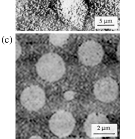
FIG. 2.: Atomic force microscope images of domains associated with boojums. Monolayers were transferred onto mica from the $L_{2}-LE$ coexistence region at a speed of 0.5mm/min (a), (c), and at 2 mm/min (b).

The good agreement between the PFM and SFM studies for the larger domains gives us confidence that the shapes have not been seriously changed during the transfer process or greatly affected by the change in substrate. We cannot be certain that this is true of the smaller domains, but it does seem likely that the effect of hydrodynamic flows and variations in the substrate will be most serious in the larger domains.

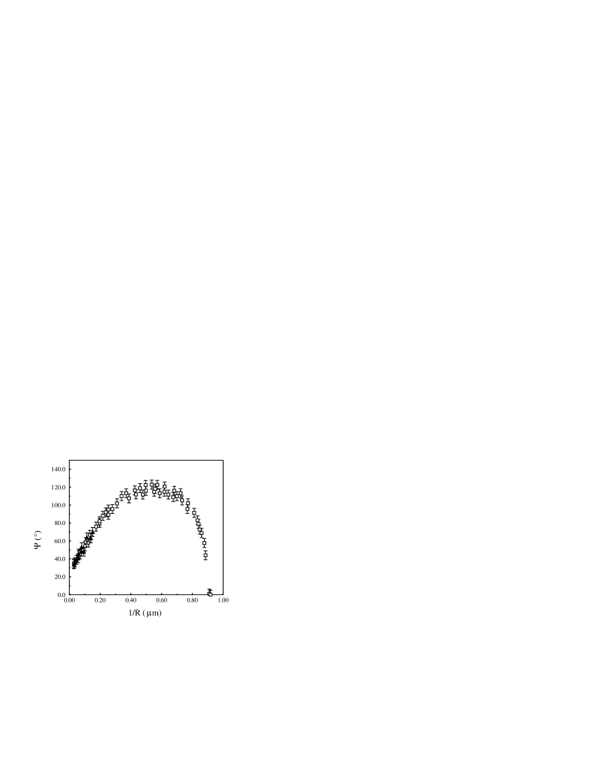
FIG. 3.: The excluded angle of the cusp-like feature on a domain supporting a boojum texture, plotted against the reciprocal of the domain radius. Filled triangles represent data for domains on water surface and empty squares represent data for domains tranferred onto solid support.

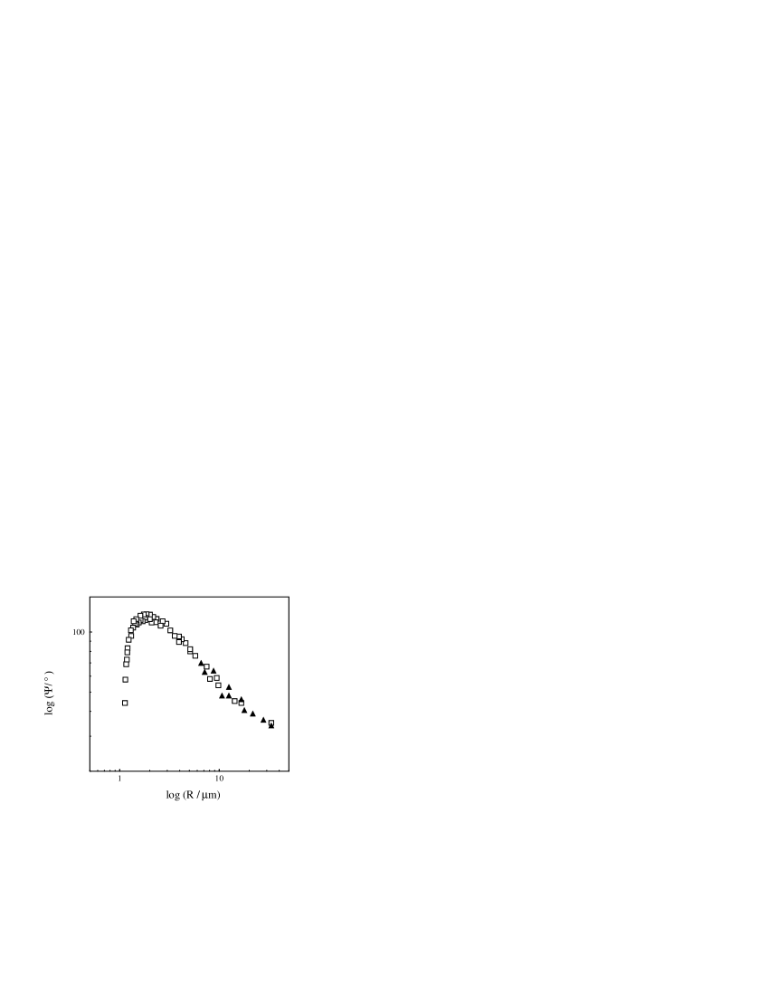
FIG. 4.: A log-log plot of the dependence on radius of the excluded angle of the cusp-like feature on a domain supporting a boojum texture. Filled triangles represent data for domains on water surface and empty squares represent data for domains tranferred onto solid support.

In the PFM studies [8] it was observed that inclusions of the $LE$ phase in the $L_{2}$ domains also had cusps. When we examined films at temperatures below the $LE$-$L_{2}$-$G$ triple point at 13^∘C[17], we found similar cusp-shaped regions in the isotropic $G$ phase surrounded by the anisotropic $L_{2}$ phase. These domains also survive transfer to a solid support. Fig. 5 is a frictional force image of such an “inverse” boojum. The frictional force within the “inverse” boojum is high because the tip images the mica substrate and not the dilute $G$ phase. This is also confirmed by the topographic image, which was obtained simultaneously. The height profile shows that the inverse boojum extends to the substrate surface.

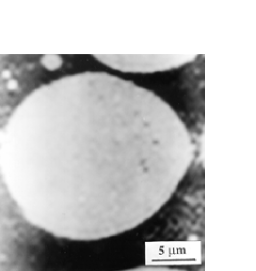
FIG. 5.: Frictional force image of an inverse boojum consisting of a bubble of the isotropic $G$ phase surrounded by the anisotropic $L_{2}$ phase. The monolayer was transferred onto mica from the $L_{2}-G$ coexistence region at a speed of 0.5 mm/min.

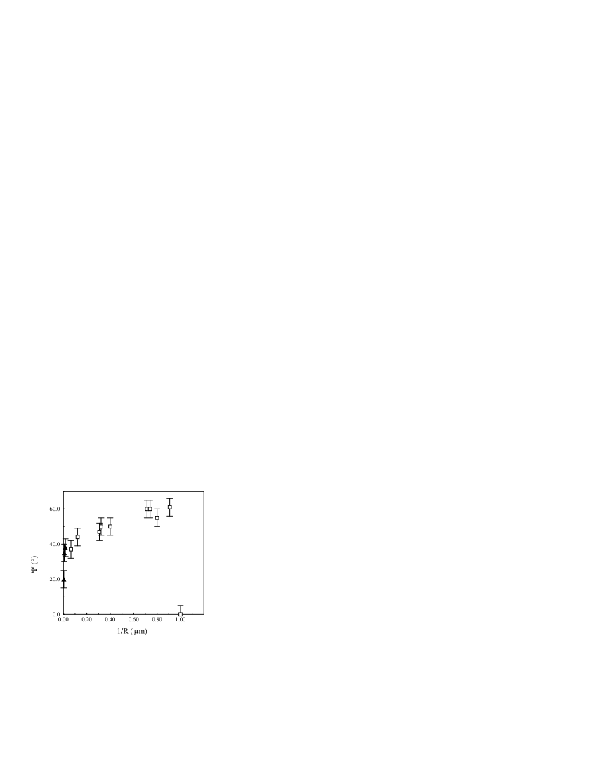
FIG. 6.: The excluded angle of the cusps in bubbles of isotropic $G$ phase surrounded by anisotropic $L_{2}$ phase, plotted versus the reciprocal of the bubble radius. filled triangles represent data for bubbles on water surface and empty squares represent data for bubbles tranferred onto solid support. Note the similarity with Fig. 3.

Measurements of the excluded angles in these inverse boojums as a function of their radii are plotted in Fig. 6. The behavior is similar to that found for the ordinary boojums; the excluded angle has a nonzero intercept, increases roughly as $R^{-0.3}$, goes through a maximum and falls to zero. Included in the figure are three points obtained from BAM studies of inverse boojums in Langmuir monolayers of pentadecanoic acid. There is a reasonable agreement with the SFM experiments for large domains. However, cusp angles are difficult to measure in small domains by BAM. They can be more easily and precisely measured by fluorescence microscopy, but the precipitation of the probe in the $L_{2}$-$G$ two-phase region made this impossible.

IV The inverse boojum

The boojum texture is an outcome of the competition between bulk and boundary energies in a bounded domain containing a condensed phase. When the boundary energy has the particular anisotropic form displayed below, and the domain is a perfect circle, this texture is an exact solution to the energy minimization equations[7]. At the same time as the $XY$-like order parameter adjusts in response to the imperatives of energy minimization, the boundary also distorts so as to accomodate the now inhomogeneous environment presented by the texture. It has been found that when the energy is as given by Eqs. (2) and (5), a circular domain satisfies the extremum equations.

This means that the simple version of the energy of a domain in a Langmuir monolayer leads to a liquid-condensed-phase domain supporting a nontrivial texture whose boundary is perfectly circular. To explain the domain shapes observed in the experiments reported here and previously [8, 9] it is necessary to introduce elaborations on the system’s energy. The addition of a higher-order harmonic term to the line tension does give rise to a distortion of the boundary [7] and a feature in the form of a cusp appears. The theory is in qualitative accord with the experiments except in the limiting large-domain behavior, where it predicts that the cusp angle vanishes rather than going to a limiting non-zero value as observed for both domains and bubbles.

The shape of bubbles of an isotropic phase inside an ordered phase was not considered in the theory. When there is a two-dimensional bubble of gas phase inside an extended region of the liquid-condensed phase a texture appears in the liquid-condensed phase that is closely related to the virtual boojum observed in two-dimensional liquid-condensed droplets. This texture minimizes the total energy $H\left[\Theta(x,y)\right]$, given by

$$H\left[\Theta(x,y)\right]= \int_{{\rm bulk}}\frac{\kappa}{2}\left|\vec{\nabla}\Theta\right|^{2}\,dxdy$$ (2)

$$+\int_{{\rm boundary}}\sigma\left(\theta-\Theta(x,y)\right)\,ds,$$

where $\Theta(x,y)$ is the angle between the vector order parameter $\hat{c}$ and the $x$-axis, while $\theta$ is the corresponding angle for the unit normal, $\hat{n}$. The coefficient $\kappa$ is the Frank, or “spin stiffness” constant. The energy above follows from the assumption of equal bend and splay moduli, which is known to represent, at best, an approximation to physical reality. The function $\sigma\left(\theta-\Theta(x,y)\right)$ is the surface energy, which depends on the relative orientations of $\hat{c}$ and the unit normal to the boundary, $\hat{n}$. The extremum equations that arise are

$$\nabla^{2}\Theta(x,y) = 0$$ (3)

$$\kappa\frac{\partial\Theta}{\partial n}+\sigma^{\prime}(\theta-\Theta) = 0$$ (4)

Eq.(3) applies outside the bubble and Eq.(4) at the interface. If $\sigma(\phi)$ has the form

$$\sigma(\phi)=\sigma_{0}+a\cos\phi,$$ (5)

and the bubble is a perfect circle, then a solution for $\Theta(x,y)$ that satisfies the extremum equations Eq. (3) and Eq. (4) is

$$\Theta(x,y)=\frac{1}{i}\left[\ln\left(1-\frac{\alpha}{x-iy}\right)-\ln\left(1-\frac{\alpha}{x+iy}\right)\right].$$ (6)

Given the similarity between the mathematical structure of the right-hand side of Eq. (6) and the expression for $\Theta(x,y)$ in the case of the virtual boojum (see ref. [7]) this solution can be characterized as an inverse boojum. It is a texture with a singularity that lies a distance $R_{B}$ from the origin, where

$$\frac{R_{B}}{R_{0}} = \frac{\alpha}{R_{0}}$$ (7)

$$= \frac{aR_{0}/\kappa}{\sqrt{1+\left(aR_{0}/\kappa\right)^{2}}+1}.$$ (8)

The above relation serves to fix the value of the quantity $\alpha$. Note that $R_{B}$ is always less than the radius of the bubble. The singularity lies within the bubble. The texture associated with a virtual boojum is displayed in Fig. 7.

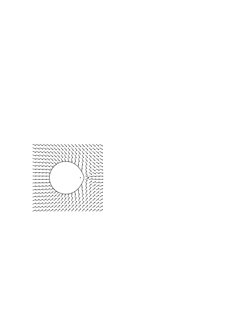
FIG. 7.: The texture associated with an inverse boojum and the position of the virtual singularity, given by Eqs. (6) and (8). The distortion of the bubble from a circle, obtained from Eq. (49), is also indicated on the Figure. The parameters used are $\kappa/a=0.4\mu m$, $a/\sigma_{0}=0.16$ and $R_{0}=2.4\mu m$.

When a virtual boojum exists in a condensed-phase domain, the orientation of the director leads to an optical anisotropy that should be observable by Brewster-angle microscopy[8, 9]. A “sunburst” of darker and lighter lines radiates from the point of singularity. Regions of constant intensity on the pattern correspond to portions of the texture in which the order parameter points in a fixed direction. In the case of the inverse virtual boojum, there should be an analogous signature of the texture in the surrounding condensed phase. Using Eq. (6) one finds straightforwardly that the orientation of the order parameter is constant along the perimeter of a circle. This means that points of equal orientation fall on circular countours as shown in Fig. 8. The contours appear to pass through two points inside the bubble. One of the points is the location of the singularity, and the other is the center of the bubble. The optical anisotropy that will be observed by BAM depends on the molecular parameters and the orientation of the boojum with respect to the direction of the incident light. Qualitative simulations of the images are shown in Fig. 9. They have been obtained by using the relation between tilt azimuth and reflectivity calculated by Tsao, et. al.[18]. These images can be compared with the BAM images in Fig. 10, which show similar variations in the reflectivity. It is interesting to note that the boojums appear to align. A similar alignment of isotropic droplets in a nematically ordered host phase has been observed[19]. This alignment is attributed to a long-range interaction produced by distortions in the director fields.

FIG. 8.: The curves along which the order parameter points in a fixed direction when there is an inverse boojum texture in the immediate vicinity of a bubble.The parameters used are $\kappa/a=0.4\mu m$, $a/\sigma_{0}=0.16$ and $R_{0}=2.4\mu m$.

V Bubble Shape: Theory

In equilibrium a bubble takes on the shape that minimizes the system’s free energy. If the interior is uniform and the line tension of an element of boundary depends on the orientation of the boundary element, the Wulff construction can be utilized to yield the shape. In the case of inhomogenous interior structure, a generalized version of the Wulff construction provides an approach to the solution[7]. This method applies to the bubble in much the same way as it does to a domain. One discovers immediately that a circular bubble does not minimize the system energy of the form (2) with $\sigma(\phi)$ given by Eq. (5), in contrast to the result obtained for a domain [7], for which a circle represents the minimum energy domain shape. However, the method cannot be applied directly because the curvature of the boundary changes sign. As a consequence, the radius of curvature of the boundary may become infinite at points along it, and this proves awkward in the context of the Wulff construction. However, a reparameterization allows one to proceed with the analysis. We find that there is no feature that can, strictly speaking, be described as a cusp, in that the slope of the bounding curve has no discontinuity. There is, on the other hand, a feature on the boundary whose shape can be quantified in terms of an excluded angle.

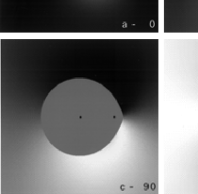
FIG. 9.: Simulated BAM images of inverse boojums for different orientations with respect to the incident light. The orientation of the beam with respect to the symmetry axis of the boojum is specified in the lower corner of each figure.

We have utilized an alternative approach to the determination of the bubble’s shape, to provide a check on our Wulff construction analysis. We adopt polar coordinates. This formulation confirms the results of the analysis based on the Wulff construction. We obtain explicit results for the bubble’s shape. Cusp angles are determined both analytically and by means of measurements on figures generated with the use of explicit analytical results, and these angles provide the basis for comparison with experiment.

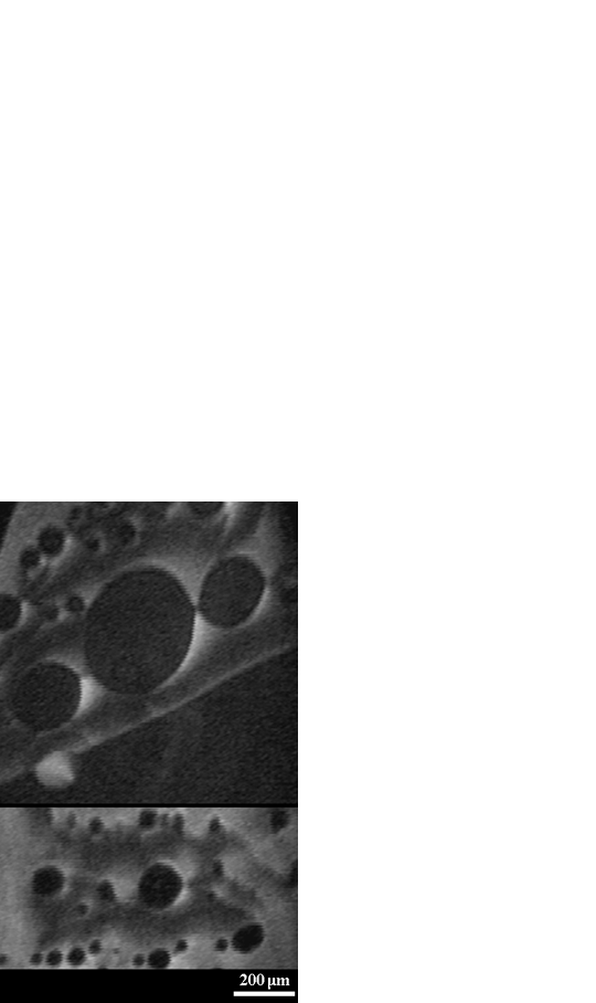
FIG. 10.: BAM images of inverse boojums in Langmuir monolayers of pentadecanoic acid at $5^{\circ}$C.

The remainder of this section consists of a review of the generalized Wulff construction, the development of the alternative approach and a summary of results. Details are deferred to a forthcoming publication[20].

A Generalized Wulff construction

Following the approach of Rudnick and Bruinsma, we attempt to apply the generalized Wulff construction [7] to determine the shape of the bubble. In our application, this technique is used to minimize the total energy Eq. (2) with respect to the Burton, Cabrera and Frank (BCF) parameterization of bubble shape, i.e. $R(\theta)$ and $\theta$ [21].

We rederive the Wulff construction so as to remove the approximation—utilized in earlier work[7]—that the radius of curvature, $R+R^{\prime\prime}$, is constant. We obtain

$$\frac{\delta}{\delta R}\int_{{\rm bulk}}\frac{\kappa}{2}\left|\vec{\nabla}\Theta\right|^{2}\,dxdy=-\frac{\kappa}{2}\left|\vec{\nabla}\Theta\right|^{2}\left[R+R^{\prime\prime}\right],$$ (9)

It can be shown that if $\sigma(\phi)=\sigma(-\phi)$, we have for the bubble

$$\frac{\delta}{\delta R}\int_{{\rm boundary}}\sigma\left(\theta-\Theta(x,y)\right)\,ds$$ (10)

$$=\sigma+\sigma^{\prime\prime}-(R+R^{\prime\prime})\left[\sigma^{\prime}(\cos\theta\frac{\partial}{\partial x}+\sin\theta\frac{\partial}{\partial y})\right.$$ (11)

$$\left.+\sigma^{\prime\prime}(-\sin\theta\frac{\partial}{\partial x}+\cos\theta\frac{\partial}{\partial y})\right]\Theta,$$ (12)

Adopting (5) and (6), the equation for the shape of the bubble is given by

$$\frac{\delta H}{\delta R}=0\Rightarrow$$ (15)

$$r+r^{\prime\prime}=$$

$$\frac{(1-2\alpha\cos\theta+\alpha^{2})^{2}}{2\alpha(\alpha+\delta)\cos 2\theta-4\alpha(1+\alpha^{2}+2\delta\alpha)\cos\theta+1+4\alpha^{2}+\alpha^{4}+\delta\alpha(1+6\alpha^{2}-\alpha^{4})},$$

where $\delta=a/\sigma_{0}$, $R=R_{0}r$ and $R_{0}$ is the radius of the unperturbed circle. The denominator of Eq. (15) passes through zero in regimes of interest, and this complicates the analysis. It proves useful to reparameterize the system in Cartesian coordinates.

The relations between the parameterization using Cartesian coordinates and the BCF parameterization are as follows:

$$x = r\sin\theta+r^{\prime}\cos\theta,$$ (16)

$$y = r\cos\theta-r^{\prime}\sin\theta.$$ (17)

Using Eq. (16) and Eq. (17), we have the following relations for nearly circular boundaries and in the region where $\theta$ is small

$$\frac{1}{r+r^{\prime\prime}} = -\frac{y^{\prime\prime}}{\sqrt{1+y^{\prime 2}}^{3}}\approx-y^{\prime\prime}$$ (18)

$$\cos\theta \approx \sqrt{1-x^{2}}\approx 1-\frac{x^{2}}{2}-\frac{x^{4}}{8}$$ (19)

Substituting Eq. (18) and Eq. (19) into Eq. (15), we obtain

$$y^{\prime\prime}=-\frac{C_{2}(x^{2}-k_{+})(x^{2}-k_{-})}{[\alpha x^{2}+(1-\alpha)^{2}]^{2}},$$ (20)

where

$$k_{\pm} = \frac{-C_{1}\pm\sqrt{C_{1}^{2}-4C_{0}C_{2}}}{2C_{2}},$$ (21)

$$C_{2} = \frac{\alpha}{2}(1+\alpha^{2}+2\delta\alpha),$$ (22)

$$C_{1} = 2\alpha(1-\alpha)^{2}-4\delta\alpha(1-\alpha),$$ (23)

$$C_{0} = (1-\alpha)^{4}+\delta\alpha(3+\alpha)(1-\alpha)^{3}.$$ (24)

The integration of Eq. (20) is readily performed easily to yield

$$y^{\prime}=$$ (25)

$$- \frac{C_{2}x}{\alpha^{2}}$$ (26)

$$- \frac{C_{2}(1-\alpha)^{4}-C_{1}\alpha(1-\alpha)^{2}+C_{0}\alpha^{2}}{2\alpha^{2}(1-\alpha)^{2}}\frac{x}{(1-\alpha)^{2}+\alpha x^{2}}$$ (27)

$$+ \frac{3C_{2}(1-\alpha)^{4}-C_{1}(1-\alpha)^{2}-C_{0}\alpha^{2}}{2(1-\alpha)^{3}\alpha^{\frac{5}{2}}}\tan^{-1}\frac{\alpha^{\frac{1}{2}}x}{1-\alpha}$$ (28)

$$+ K_{y^{\prime}},$$ (29)

and

$$y = -\frac{C_{2}x^{2}}{2\alpha^{2}}-\frac{2(1-\alpha)^{2}+C_{1}\alpha}{2\alpha^{3}}\ln[\alpha x^{2}+(1-\alpha)^{2}]$$ (32)

$$+\frac{3C_{2}(1-\alpha)^{4}-C_{1}(1-\alpha)^{2}-C_{0}\alpha^{2}}{2(1-\alpha)^{3}\alpha^{\frac{5}{2}}}x\tan^{-1}\frac{\alpha^{\frac{1}{2}}x}{1-\alpha}$$

$$+K_{y^{\prime}}x+K_{y}.$$

The next step is to fix the constants of integration $K_{y^{\prime}}$ and $K_{y}$. Symmetry requires $y^{\prime}(-x)=-y^{\prime}(x)$, and yields $K_{y^{\prime}}=0$. The bounding curve $y(x)$ will merge into a circle of radius 1, centered at the origin. The merging point, $(x_{0},y(x_{0}))$, is taken to be the point at which $y^{\prime}(x_{0})=-x_{0}/\sqrt{1-x_{0}^{2}}$. This leads to

$$K_{y}=$$ (33)

$$\frac{C_{2}x_{0}^{2}}{2\alpha^{2}}+\frac{2(1-\alpha)^{2}+C_{1}\alpha}{2\alpha^{3}}\ln[\alpha x_{0}^{2}+(1-\alpha)^{2}]$$ (34)

$$-\frac{3C_{2}(1-\alpha)^{4}-C_{1}(1-\alpha)^{2}-C_{0}\alpha^{2}}{2(1-\alpha)^{3}\alpha^{\frac{5}{2}}}x_{0}\tan^{-1}\frac{\alpha^{\frac{1}{2}}x_{0}}{1-\alpha}$$ (35)

$$+\sqrt{1-x_{0}^{2}},$$ (36)

The boundary of the bubble Eq. (32) is smooth in that there is no discontinuity in the slope of the bounding curve. For very small $R_{0}$, the radius of curvature of the boundary close to the virtual boojum, $b=1/y^{\prime\prime}(0)$, is approximately equal to $R_{0}$. The bubble appears to be circular and the excluded angle, $\Psi$, is zero. The ratio $\beta=b/R_{0}$ decreases as $R_{0}$ increases. This causes the bubble to sharpen at one end. When $\beta$ exceeds a critical value $\beta_{c}$, this sharper end has properties in common with be a cusp, and one is able to derive a excluded angle, $\Psi$, as depicted in Fig. 11a. It can be shown that $\Psi$ is given by the following:

$$\Psi=2\cos^{-1}\frac{1}{1+\frac{h}{1-b}},$$ (37)

where $h=|y(0)+1|$is the deviation of the tip of the feature from a circle. Because there never a cusp in the strict sense of the term the choice of $\beta_{c}$, is a matter of individual judgement. Based on theoretical bubble shapes obtained in Fig. 12, $\beta_{c}$ is chosen to be $0.45$.

When $R_{0}\gg\kappa/a$, the $x^{2}$ term in Eq. (29) dominates. The boundary around the cusp-like feature is this $x^{2}$ term instead of the unperturbed circle. The new definition of the excluded angle is as displayed in Fig. 11b and we find $\Psi$ can be expressed as

$$\Psi\approx 2\sqrt{2\left|\frac{2(1-\alpha)^{2}+C_{1}\alpha}{\alpha^{3}}\ln(1-\alpha)\right|}.$$ (38)

In this limit, $\alpha\rightarrow 1-\epsilon$, where $\epsilon\propto r^{-1}\ll 1$, we approximate $C_{1}$ as follows

$$C_{1}\approx 2\epsilon(\epsilon-2\delta)+O(\delta\epsilon^{2}),$$ (39)

We then have the large-$R_{0}$ behaviour of the excluded angle

$$\Psi\approx 2\sqrt{\frac{8\kappa}{\sigma_{0}R_{0}}\left|\ln\frac{\kappa}{aR_{0}}\right|}$$ (40)

FIG. 11.: (a) The way in which $\Psi$ is defined where the boundary is smooth. This method leads to an analytical expression for the excluded angle of a cusp-like feature. (b) For $R_{0}\gg\kappa/a$, the ”cusp”-like feature show up differently and requires a new definition of $\Psi$.

B Polar Coordinates

As an alternative, one can parameterize the domain boundary in polar coordinates. In this case, we choose an origin, nominally at the center of the undistorted circular bubble. The cartesian coordinates $x$ and $y$ are replaced by $r$, the distance from the origin and $\phi$, the angle with respect to the $x$ axis. In terms of $r$ and $\phi$, the inverse boojum texture has the form

$$\Theta\left(r,\phi\right)=\frac{1}{i}\left[\ln\left(1-\frac{\alpha}{r}e^{i\phi}\right)-\ln\left(1-\frac{\alpha}{r}e^{-i\phi}\right)\right].$$ (41)

The boundary condition, Eq. (4) leads to the following result for the parameter $\alpha$:

$$\frac{\alpha}{R_{0}}=\frac{1}{\sqrt{\left(\kappa/\alpha R_{0}\right)^{2}+1}+\left(\kappa/\alpha R_{0}\right)},$$ (42)

where $R_{0}$ is the radius of the circular bubble. The parameter $\alpha$ has a simple interpretation—it is the distance of the singularity associated with the virtual boojum from the center of the bubble. Note that according to Eq. (42) the singularity always lies within the bubble.

We now proceed with a calculation of the distortion of the bubble from a circle. Our results are the leading order terms in an expansion in the dimensionless, and presumably small, combination $a/\sigma_{0}$. If one writes

$$r(\phi)=R_{0}e^{k(\phi)},$$ (43)

one eventually arrives at

$$R_{0}\sigma_{0}k^{\prime\prime}(\phi)=$$ (44)

$$-a\alpha\left[\frac{\left(e^{i\phi}-\frac{\alpha}{R_{0}}\right)e^{i\phi}}{\left(1-\frac{\alpha}{R_{0}}e^{i\phi}\right)^{2}}+\frac{\left(e^{-i\phi}-\frac{\alpha}{R_{0}}\right)e^{-i\phi}}{\left(1-\frac{\alpha}{R_{0}}e^{-i\phi}\right)^{2}}\right]$$ (45)

$$-\frac{2\kappa\left(\frac{\alpha}{R_{0}}\right)^{2}}{\left(1-\frac{\alpha}{\rho}e^{i\phi}\right)\left(1-\frac{\alpha}{\rho}e^{-i\phi}\right)}.$$ (46)

Eq. (46) represents the leading term in an expansion in the dimentionless combination $a/\sigma_{0}$. This ratio is small, as the line tension is assumed to be nearly isotropic.

The double integration of Eq. (46) is relatively straightforward. One finds for $k(\phi)$:

$$k(\phi) = \frac{2\kappa}{\sigma_{0}R_{0}}\left[2\int_{-\pi}^{\phi}\arctan\left(\frac{\frac{\alpha}{R_{0}}\sin\phi^{\prime}}{1-\frac{\alpha}{R_{0}}\cos\phi^{\prime}}\right)d\phi^{\prime}\right.$$ (49)

$$-\ln\left(1+\left(\frac{\alpha}{R_{0}}\right)^{2}-2\frac{\alpha}{R_{0}}\cos\phi\right)$$

$$\left.+2\ln\left(1+\frac{\alpha}{R_{0}}\right)\right].$$

FIG. 12.: (a) The calculated shapes for the bubble of $R_{0}$=0.4, 0.8, 1, 1.2, 1.6, 2, 2.4 and 3.2 $\mu m$. The bubble which is drawn in thicker line is the one of the nominal size, $R_{c}=1\mu m$ when $\beta_{c}=0.45$ for this case. (b) The calculated shapes for the bubbles of $R_{0}$=3.2, 8 and 16 $\mu m$. The parameters used are $\kappa/a=0.4\mu m$ and $a/\sigma_{0}=0.16$.

In the regimes in which comparisons can be made, the results of the calculation based on the utilization of polar coordinates are in complete accord with results that follow from the Wulff construction. In addition, an analysis based on polar coordinates—in particular Eq.( 49)—provides figures that can be utilized for comparison with experimental data. Bubbles whose shapes are described by Eq. (43) and Eq. (49) are displayed in Fig. 12. These bubbles comprise the results of theoretical modeling that are compared with the data described in earlier sections.

VI Results and conclusions

We now compare the theoretical excluded angles with the experimental ones. Within the range of experiment data, Eq. (37) provides the basis for comparison between experiments and theory. We find that the best fit is achieved when the parameters are chosen as $\kappa/a=0.4\mu m$ and $a/\sigma_{0}=0.16$. The comparison between theory and experiment is displayed in Fig. 13. Because of the fact that there is never a cusp in the form of a discontinuity in the slope of the bounding curve, we are unable to definitively model the “onset” of a cusp. However, we do find an apparent rapid dropoff to zero of the (nominal) excluded angle. Furthermore, the theory predicts that sufficiently small bubbles will be nearly circular. It is possible to determine a value of what appears to be the radius of onset, $R_{c}$, with the exercise of a little judgement. For the parameters of choice, we find $R_{c}=1\mu m$ for $\beta_{c}=0.45$.

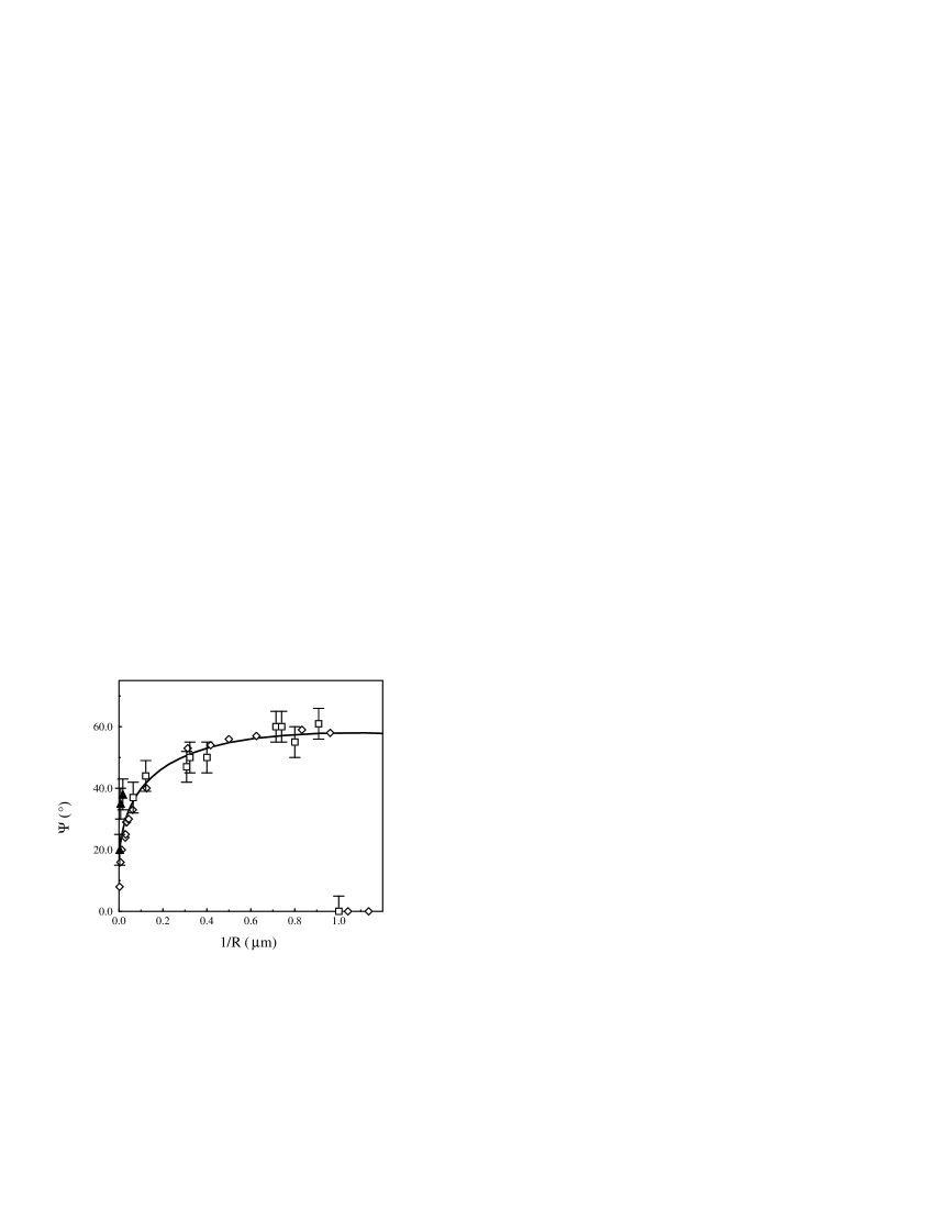
FIG. 13.: The experimental measured excluded angle of the cusps in bubbles, as in Fig. 6, shown as empty squares and filled triangles, the measured excluded angle of the calculated bubbles shown as empty diamond and the analytic expression of the theoretical excluded angle shown as solid line, plotted vesus the reciprocal of the bubble radius. Note the fundamental difference between the behavior of the the small-radius behavior of the theoretical curve, which tends monotonically to a finite limit at vanishing bubble radius and the measured excluded angle of calculated bubbles, which seems to rise rapidly from zero as the bubble radius exceeds a “threshold” value.

Our theory appears to reproduce fairly well both the qualitative and the quantitative behaviour of the bubble shapes as a function of the bubble size. Small bubbles are nearly circular and the excluded angle, $\Psi$, is equal to zero. Cusp-like features are observed for bubbles having radii $R_{0}$ greater than a threshold value $R_{c}$. The angle $\Psi$ decreases for bubbles of larger sizes. However, in the experiments,the excluded angle $\Psi$ tends to a non-zero constant as $R_{0}\rightarrow\infty$. This limiting behavior is not achievable within the framework of the theory presented here. It is known that thermal fluctuations will cause the line tension coefficients to depend on the diameter of the bubble or domain[23]. However, preliminary calculations indicate that this renormalization has no effect on the asymptotic behavior of the excluded angle for large domains of bubbles. A possible source of the discrepancy is the difference between the bend and splay moduli, which has been neglected in the present work.

The ratio $\kappa/a$ for hexadecanoic acid has been obtained by Rivière and Meunier [9]. They find $28\mu m<\kappa/a<40\mu m$, about two orders of magnitude larger from our best estimate, $\kappa/a=0.4\mu m$. Studies of other textures in monolayers such as stripes[24] indicate that $\kappa$ increases with chain length. This could account for some of the difference. Another possible reason for this discrepancy is the fact that Rivière and Meunier adopted $\kappa_{1}\neq\kappa_{3}$ as the basis for texture distortions while we have used $a$, the anisotropic line tension, as the mechanism for bubble shape distortions. Our comparison between theory and experiment gives an estimate of $a/\sigma_{0}=0.16$ for pentadecanoic acid at $LC$-$G$ boundary. The line tension anisotropy, which corresponds to of our $a/\sigma_{0}$, has been estimated for the $LC$-$LE$ interface in D-myristoyl alanine from studies of dendritic growth[25]. The value found is 0.005 - 0.025. Given the fact that the systems are not identical, and that these are only estimates of the anisotropy, the difference is not at all disturbing.

In summary, we have formulated a theory for bubbles in Langmuir monolayers that is an extension and reformulation of the theory of domain shapes discussed by Rudnick and Bruinsma [7]. Although the current theory predicts a smooth bubble boundary, there exist cusp-like features with well-defined and measurable excluded angles when the radius of the bubble exceeds a nominal value $R_{c}$. Comparing theoretical excluded angles with the results of experiments, we find good qualitative and quantitative agreement. However, there are also discrepancies. Experimental observations and related work indicate that the difference between $\kappa_{1}$ and $\kappa_{3}$ cannot be neglected. The calculation of an equilibrium texture when $\kappa_{1}\neq\kappa_{3}$ is currently being performed as a prelude to the determination of the shape of a bubble or domain.

REFERENCES

- [1] V. T. Moy, D. J. Keller, H. E. Gaub and H. M. McConnell, J. Phys. Chem. 90, 3198 (1986); D. K. Schwartz and C. M. Knobler, J. Phys. Chem. 97, 8849 (1993).
- [2] S. Hénon and J. Meunier, Rev. Sci. Instrum. 62, 936 (1991); D. Hönig and D. Möbius, J. Phys. Chem. 95, 4590 (1991).
- [3] T. Fischer, C. M. Knobler and R. Bruinsma, Phys. Rev. E 50, 423 (1994).
- [4] For a description of monolayer phases see C. M. Knobler and R.C. Desai, Ann. Rev. Phys. Chem. 43, 207 (1992).
- [5] S. A. Langer and J. P. Sethna, Phys. Rev. A 34, 5035 (1986). For the original discussion of boojums, see N. D. Mermin in Quantum Fluids and Solids, S. B. Trickey, E. Adams and J. Duffy, eds. (Plenum, New York, 1977).
- [6] G. Wulff, Z. Kristalogr. 34, 449 (1901); M. Wortis in Chemistry and Physics of Solid Surfaces VII, edited by R. Vanselow and R. Howe (Springer Verlag Berlin, 1988), p. 367.
- [7] J. Rudnick and R. Bruinsma, Phys. Rev. Lett. 74, 2491 (1995).
- [8] D. K. Schwartz, M.-W. Tsao and C. M. Knobler, J. Chem. Phys. 101, 8258 (1994).
- [9] R. Rivière and J. Meunier, Phys. Rev. Lett. 74, 2495 (1995).
- [10] P. Galatola and J. B. Fournier, Phys. Rev. Lett. 75, 3297 (1995).
- [11] B. Fischer, M.-W. Tsao, J. Ruiz-Garcia, T. M. Fischer and C. M. Knobler, J. Phys. Chem. 98, 7430 (1994).
- [12] L. F. Chi, M. Anders, H. Fuchs, R. R. Johnston and H. Ringsdorf, Science 259, 213 (1993).
- [13] J. M. Mikrut, P. Dutta, J. B. Ketterson and R. C. MacDonald, Phys. Rev. B 48, 14479 (1993) .
- [14] J. Y. Fang and C. M. Knobler, J. Phys. Chem. 99, 10425 (1995).
- [15] S. Schwiegk, T. Vahlenkamp, Y. -Z. Xu and G. Wegner, Macromolecules 25, 2513 (1992).
- [16] J. Y. Fang, Z. H. Lu, G. W. Min, Z. M. Ai,Y. Wei and P. Stroeve, Phys. Rev. A 46, 4963 (1992).
- [17] B. G. Moore, C. M. Knobler, S. Akamatsu and F. Rondelez, J. Phys. Chem. 94, 4588 (1990).
- [18] M.-W. Tsao, T. M. Fischer and C. M. Knobler, Langmuir, 11, 3184 (1995).
- [19] P. Poulin, H. Stark, T. C. Lubensky and D. A. Weitz, preprint.
- [20] K. K. Loh and J. Rudnick, in preparation.
- [21] W. K. Burton, N. Cabrera and F. C. Frank, Philos. Trans. Roy. Soc. 243, 291 (1951).
- [22] L. Santesson, T. M. H. Wong, M. Taborelli, P. Descouts, M. Liley, C. Duschl, H. Vogel, J. Phys. Chem. 99, 1038 (1995).
- [23] H. Saleur and P. Fendley, private communication.
- [24] J. Ruiz-Garcia, X. Qiu, M.-W. Tsao, G. Marshall and C. M. Knobler, J. Phys. Chem. 97, 6955 (1993).
- [25] S. Akamatsu, O. Bouloussa, K. To and F. Rondelez, Phys. Rev. A 46, 4504 (1992).