Introduction To Monte Carlo Algorithms

Abstract

In these lectures, given in ’96 summer schools in Beg-Rohu (France) and Budapest, I discuss the fundamental principles of thermodynamic and dynamic Monte Carlo methods in a simple light-weight fashion. The keywords are Markov chains, Sampling, Detailed Balance, A Priori Probabilities, Rejections, Ergodicity, “Faster than the clock algorithms”.

The emphasis is on Orientation, which is difficult to obtain (all the mathematics being simple). A firm sense of orientation helps to avoid getting lost, especially if you want to leave safe trodden-out paths established by common usage.

Even though I will remain quite basic (and, I hope, readable), I make every effort to drive home the essential messages, which are easily explained: the crystal-clearness of detail balance, the main problem with Markov chains, the great algorithmic freedom, both in thermodynamic and dynamic Monte Carlo, and the fundamental differences between the two problems.

Chapter 1 Equilibrium Monte Carlo methods

1.1 A Game in Monaco

The word “Monte Carlo method” can be traced back to a game very popular in Monaco. It’s not what you think, it’s mostly a children’s pass-time played on the beaches. On Wednesdays (when there is no school) and on weekends, they get together, pick up a big stick, draw a circle and a square as shown in figure 1.1. They fill their pockets with pebbles

Figure 1.1: Children at play on the beaches of Monaco. They spend their afternoons calculating $\pi$ by a method which can be easily extended to general integrals.

. Then they stand around, close their eyes, and throw the pebbles randomly in the direction of the square. Someone keeps track of the number of pebbles which hit the square, and which fall within the circle (see figure 1.1). You will easily verify that the ratio of pebbles in the circle to the ones in the whole square should come out to be $\pi/4$, so there is much excitement when the $40$th, $400$th, $4000$th is going to be cast.

This breath-taking game is the only method I know to compute the number $\pi$ to arbitrary precision without using fancy measuring devices (meter, balance) or advanced mathematics (division, multiplication, trigonometry). Children in Monaco can pass the whole afternoon at this game. You are invited to write a little program to simulate the game. If you have never written a Monte Carlo program before, this will be your first one. You may also recover “simplepi.f” from my WWW-site.

Lately, big people in Monaco have been getting into a similar game. Late in the evenings, when all the helicopters are safely stowed away,

Figure 1.2: Adults at play on the Monte Carlo heliport. Their method to calculate $\pi$ has been extended to the investigation of liquids, suspensions, and lattice gauge theory.

they get together on the local heliport (cf. figure 1.2), which offers the same basic layout as in the children’s game. They fill their expensive Hermès handbags with pebbles, but since the field is so large, they play a slightly different game: they start somewhere on the field, close their eyes, and then throw the little stone in a random direction. Then they walk to where the first stone landed, take a new one out of their handbag, and start again. You will realize that using this method, one can also sweep out evenly the heliport square, and compute the number $\pi$. You are invited to write a $10$-line program to simulate the heliport game - but it’s not completely trivial.

Are you starting to think that the discussion is too simple? If that is so, please consider the lady at c). She just flung a pebble to c’), which is outside the square. What should she do?

1. simply move on at c)

2. climb over the fence, and continue until, by accident, she will reintegrate the heliport

3. other:  

A correct answer to this question will be given on page 1.6, it contains the essence of the concept of detailed balance. Many Monte Carlo programs are wrong because the wrong alternative was programmed.

The two cases - the children’s game and the grown-ups’ game are perfect illustrations of what is going on in Monte Carlo…and in Monte Carlo algorithms. In each case, one is interested in evaluating an integral

$$\int_{x,y\;\epsilon\framebox[5.69046pt]{}}dxdy\pi(x,y)f(x,y)$$ (1.1)

with a probability density $\pi$ which, in our case is the square

$$\pi(x,y)=\left\{\begin{array}[]{ll}1&\mbox{if $|x|<1$ and $|y|<1$}\\ 0&\mbox{otherwise}\end{array}\right.$$ (1.2)

and a function $f$ (the circle)

$$f(x,y)=\left\{\begin{array}[]{ll}1&\mbox{if $x^{2}+y^{2}<1$}\\ 0&\mbox{otherwise}\end{array}\right.$$ (1.3)

Both the children and the grown-ups fill the square with a constant density of pebbles (corresponding to $\pi(x,y)=1.)$, one says that they sample the function $\pi(x,y)$ on the basic square. If you think about it you will realize that the number $\pi$ can be computed in the two games only because the area of the basic square is known. If this is not so, one is reduced to computing the ratio of the areas of the circle and of the square, i.e., in the general case, the ratio of the integrals:

$$\int_{x,y\;\epsilon\framebox[5.69046pt]{}}dxdy\pi(x,y)f(x,y)/\int_{x,y\;\epsilon\framebox[5.69046pt]{}}dxdy\pi(x,y)$$ (1.4)

Two basic approaches are used in the Monte Carlo method:

1. direct sampling (children on the beach)

2. Markov-chain sampling (adults on the heliport)

Direct sampling is usually like Pure Gold, it means that you are able to call a subroutine which provides an independent hit at your distribution function $\pi(x,y)$. This is exactly what the kids do whenever they get a new pebble out of their pockets.

Most often, there is no way to do direct sampling in a reasonable manner. One then resorts to Markov-chain sampling, as the adults on the heliport. Almost all physical systems are of this class. A famous example, which does not oblige us to speak of energies, hamiltonians etc. has occupied more than a generation of physicists. It can easily be created with a shoe-box, and a number of coins (cf figure 1.3): how do you generate (directly sample)

Figure 1.3: The Coin in a shoe-box problem (hard disks) has occupied Monte Carlo workers since 1953. There is no direct-sampling algorithm, and Markov-chain sampling is extremely tedious at some densities.

random configurations of the coins such that they don’t overlap? Imagine the $2N$-dimensional configuration space of $N$ non-overlapping coins in a shoe-box. Nobody has found a subroutine which would directly sample this configuration space, i.e. create any of its members with equal probability. First-time listeners often spontaneously propose a method called Random Sequential Adsorption: deposit a first coin at a random position, then a second, etc, (if they overlap, simply try again). Random Sequential Adsorption will be dealt with in detail, but in a completely different context, on page 2.5. Try to understand that this has nothing to do with finding a random non-overlapping configuration of the coins in the shoe-box (in particular, the average maximum density of random sequential deposition is much smaller than the close packing density of the coins).

Direct sampling is usually impossible - and that is the basic frustration of Monte Carlo methods (in statistical physics). In contrast, the grown-ups’ game can be played in any situation (…already on the heliport which is too large for direct sampling). Markov chain sampling has been used in an uncountable number of statistical physics models, in the aforementioned coin-in-a-box problem, the Hubbard model, etc etc. Usually it is a very poor, and extremely costly substitute to what we really want to do.

In the introduction, I have talked about Orientation, and to get oriented you should realize the following:

• In the case of the children’s game, you need only a few dozen pebbles (samples) to get a physicist’s idea of the value of $\pi$, which will be sufficient for most applications. Exactly the same is true for some of the most difficult statistical physics problems. A few dozen (direct) samples of large coin-in-the-box problems at any density would be sufficient to resolve long-standing controversies. (For a random example, look up ref. [14], where the analysis of a monumental simulation relies on an effective number of $4-5$ samples).

  Likewise, a few dozen direct samples of the Hubbard model of strong fermionic correlation would give us important insights into superconductivity. Yet, some of the largest computers in the world are churning away day after day on problems as the ones mentioned. They all try to bridge the gap between the billions of Markov chain samples and the equivalent of a few random flings in the children’s game.

• It is only after the problem to generate independent samples by Markov chains at all is understood, that we may start to worry about the slow convergence of mean-values. This is already apparent in the children’s game - as in every measurement in experimental physics - : the precision of the numerical value decreases only as $1/\sqrt{N}$, where $N$ is the number of independent measurements. Again, let me argue against the “mainstream” that the absolute precision discussion is not nearly as important as it may seem: you are not always interested in computing your specific heat to five significant digits before putting your soul to rest. In daily practice of Monte Carlo it is usually more critical to be absolutely sure that the program has given some independent samples rather than that there are millions and billions of them.

• It is essential to understand that a long Markov chain, even if it produces only a small number of independent samples (and thus a very approximative result) is usually extremely sensitive to bugs, and even small irregularities of the program.

1.2 The Toddlers’ algorithm and detailed balance

We have yet to determine what the lady at point c) in the heliport game should do. It’s a difficult question, and full of consequences, and we don’t want to give her any wrong advice. So, let’s think, and analyze first a similar, discretized game, the well-known puzzle shown in figure 1.4. Understanding this puzzle will allow us to make a definite recommendation.

Figure 1.4: This well-known puzzle is the starting point for our theoretical analysis of the Monte Carlo method.

The task is now to create a perfect scrambling algorithm which generates any possible configuration of the puzzle with equal probability. One such method, the toddlers’ algorithm, is well known, and illustrated in figure 1.5 together with one of its inventors.

Figure 1.5: This is a direct sampling algorithm for the puzzle game.

The theoretical baggage picked up in the last few sections allows us to class this method without hesitation among the direct sampling methods (as the children’s game before), since it creates an independent instance each time the puzzle is broken apart.

We are rather interested in a grown-up people’s algorithm, which respects the architecture of the game .

What would You do? Almost certainly, you would hold the puzzle in your hands and - at any time step - move the empty square in a random direction. The detailed balance condition which you will find out about in this section shows that this completely natural sounding algorithm is wrong.

If the blank square is in the interior (as in figure 1.4) then the algorithm should clearly be to choose one of the four possible directions  $\uparrow$  $\rightarrow$  $\downarrow$  $\leftarrow$ with equal probability, and to move the empty square.

As in the heliport game, we have to analyze what happens at the boundary of the square .

Figure 1.6: The corner configuration $a$ is in contact with the configurations $b$ and $c$

Consider the corner configuration $a$, which communicates with the configurations $b$ and $c$, as shown in figure 1.6. If our algorithm (yet to be found) generates the configurations $a$, $b$ and $c$ with probabilities $\pi(a)$, $\pi(b)$, and $\pi(c)$, respectively (we impose them to be the same), we can derive a simple rate equation relating the $\pi$’s to the transition probabilities $p(a\rightarrow b)$ etc. Since $a$ can only be generated from $b$, $c$, or from itself, we have

$$\pi(a)=\pi(b)p(b\rightarrow a)+\pi(c)p(c\rightarrow a)+\pi(a)p(a\rightarrow a)$$ (1.5)

this gives

$$\pi(a)[1-p(a\rightarrow a)]=\pi(b)p(b\rightarrow a)+\pi(c)p(c\rightarrow a)$$ (1.6)

We write the condition which tells us that the empty square, once at $a$, can stay at $a$ or move to $b$ or $c$:

$$1=p(a\rightarrow a)+p(a\rightarrow b)+p(a\rightarrow c)$$ (1.7)

which gives $[1-p(a\rightarrow a)]=p(a\rightarrow b)+p(a\rightarrow c)$. This formula, introduced in eq. (1.6) yields

$$\pi(a)\underbrace{p(a\rightarrow b)+\pi(a)\overbrace{p(a\rightarrow c)=\pi(c)}p(c\rightarrow a)+\pi(b)}p(b\rightarrow a)$$ (1.8)

We can certainly satisfy this equation if we equate the braced terms separately:

$$\pi(a)p(a\rightarrow b)=\pi(b)p(b\rightarrow a)\;\;\mbox{etc.}$$ (1.9)

This equation is the celebrated Condition of detailed Balance.

We admire it for awhile, and then pass on to its first application, in our puzzle. There, we impose equal probabilities for all accessible configurations, i. e. $p(a\rightarrow b)=p(b\rightarrow a)$, etc, and the only simple way to connect the proposed algorithm for the interior of the square with the boundary is to postulate an equal probability of $1/4$ for any possible move. Looking at eq. (1.7), we see that we have to allow a probability of $1/2$ for $p(a\rightarrow a)$. The consequence of this analysis is that to maximally scramble the puzzle, we have to be immobile with a probability $1/2$ in the corners, and with probability $1/4$ on the edges.

We can assemble all the different rules in the following algorithm: At each time step $t=0,1,\ldots$

1. choose one of the four directions  $\uparrow$  $\rightarrow$  $\downarrow$  $\leftarrow$ with equal probability.

2. move the blank square into the corresponding direction if possible. Otherwise, stay where you are, but advance the clock.

I have presented this puzzle algorithm in the hope that you will not believe that it is true. This may take you to scrutinize the detailed balance condition, and to understand it better.

Recall that the puzzle game was in some respect a discretized version of the heliport game, and you will now be able to answer by analogy the question of the fashionable lady at c). Notice that there is already a pebble at this point. The lady should now pick two more stones out of her handbag, place one of them on top of the stone already on the ground, and use the remaining one to try a new fling. If this is again an out-fielder, she should pile one more stone up etc. If you look onto the heliport after the game has been going on for awhile, you will notice a strange pattern of pebbles on the ground (cf. figure 1.7).

Figure 1.7: Landing pad of the Monte Carlo heliport after all the players have gone home. Notice the piles at the edges, particularly close to the corners.

There are mostly single stones in the interior, and some more or less high piles as you approach the boundary, especially the corner. Yet, this is the most standard way to enforce a constant density $\pi(x,y)=const$.

It has happened that first-time listeners of these sentences are struck with utter incredulity. They find the piling-up of stones absurd and conclude that I must have gotten the story wrong. The only way to reinstall confidence is to show simulations (of ladies flinging stones) which do and do not pile up stones on occasions. You are invited to do the same (start with one dimension).

In fact, we have just seen the first instance of a Rejection, which, as announced, is a keyword of this course, and of the Monte Carlo method in general. The concept of a rejection is so fundamental that it is worth discussing it in the completely barren context of a Monaco airfield. Rejections are the basic method by which the Monte Carlo enforces a correct density $\pi(x,y)$ on the square, with an algorithm (random “flings”) which is not particularly suited to the geometry. Rejections are also wasteful (of pebbles), and expensive (you throw stones but in the end you just stay where you were). We will deepen our understanding of rejections considerably in the next sections.

We have introduced the rejections by a direct inspection of the detailed balance condition. This trick has been elevated to the status of a general method in the socalled Metropolis algorithm [1]. There, it is realized that the detailed balance condition eq. (1.9) is verified if one uses

$$P(a\rightarrow b)=\min(1,\frac{\pi(b)}{\pi(a)})$$ (1.10)

What does this equation mean? Let’s find out in the case of the heliport: Standing at a) (which is inside the square, i.e. $\pi(a)=1$), you throw your pebble in a random direction (to $b$). Two things can happen: Either $b$ is inside the square ($\pi(b)=1$), and eq. (1.10) tells you to accept the move with probability $1$, or $b$ is outside ($\pi(b)=0$), and you should accept with probability $0$, i.e. reject the move, and stay where you are.

After having obtained an operational understanding of the Metropolis algorithm, you may want to see whether it is correct in the general case. For once, there is rescue through bureaucracy, for the theorem can be checked by a bureaucratic procedure: simply fill out the following form:

case	$\pi(a)>\pi(b)$	$\pi(b)>\pi(a)$
$P(a\rightarrow b)$			$1$
$\pi(a)P(a\rightarrow b)$			$2$
$P(b\rightarrow a)$			$3$
$\pi(b)P(b\rightarrow a)$			$4$

Fill out, and you will realize for both columns that the second and forth rows are identical, as stipulated by the detailed balance condition. You have understood all there is to the Metropolis algorithm.

1.3 To Cry or to Cray

Like a diamond tool, the Metropolis algorithm allows you to “grind down” an arbitrary density of trial movements (as the random stone-flings) into the chosen stationary probability density $\pi(x,y)$.

To change the setting we discuss here how a general classical statistical physics model with an arbitrary high-dimensional energy $E(x_{1},x_{2},\ldots,x_{N}$) is simulated (cf the classic reference [2]). In this case, the probability density is the Boltzmann measure $\pi(x_{1},...,x_{N})=\exp(-\beta E)$, and the physical expectation values (energies, expectation values) are given by formulas as in eq. (1.4). All you have to do (if the problem is not too difficult) is to …

• set up a (rather arbitrary) displacement rule, which should generalize the random stone-flings of the heliport game. For example, you may from an initial configuration $x_{1},x_{2},\ldots,x_{N}$ go to a new configuration by choosing an arbitrary dimension i, and doing the random displacement on $x_{i}\rightarrow x_{i}+\delta x$, with $\delta x$ between $-\epsilon$ and $+\epsilon$. Discrete variables are treated just as simply.

• Having recorded the energies $E^{a}$ and $E^{b}$ at the initial point $a$ and the final point $b$, you may use the Metropolis algorithm to compute the probability, $p$, to actually go there.

  $$p(a\rightarrow b)=\min[1,\exp(-\beta(E^{b}-E^{a})])$$ (1.11)

  This is implemented using a single uniformly distributed random number $0<ran<1$, and we move our system to $b$ under the condition that $ran<p(a\rightarrow b)$, as shown in the figure.

  Figure 1.8: The probability for a uniformly distributed random number $0<ran<1$ to be smaller than $p(a\rightarrow b)$ is $\min[1,p(a\rightarrow b)]$. A typical Monte Carlo program contains one such comparison per step.

• You notice that (for continuous systems) the remaining liberty in your algorithm is to adjust the value of $\epsilon$. The time-honored procedure consists in choosing $\epsilon$ such that about half of the moves are rejected. This is of course just a golden rule of thumb. The “$<p(\epsilon)>\sim 1/2$” rule, as it may be called, does in general insure quite a quick diffusion of your particle across configuration space. If you want to do better, you have to monitor the speed of your Monte Carlo diffusion, but it is usually not worth the effort.

As presented, the Metropolis algorithm is extremely powerful, and many problems are adequately treated with this method. The method is so powerful that for many people the theory of Monte Carlo stops right after equation (1.9). All the rest is implementation details, data collection, and the adjustment of $\epsilon$, which was just discussed.

Many problems, especially in high dimensions, nevertheless defy this rule. For these problems, the programs written along the lines of the one presented above will run properly, but have a very hard time generating independent samples at all. These are the problems on which one is forced to either give up or compromise: use smaller sizes than one wants, take risks with the error analysis etc. The published papers, over time, present much controversy, shifting results, and much frustration on the side of the student executing the calculation.

Prominent examples of difficult problems are phase transitions in general statistical models, Hubbard model, Bosons, and disordered systems. The strong sense of frustration can best be retraced in the case of the hard sphere liquid, which was first treated in the original $1953$ publication introducing the Metropolis algorithm, and which has since generated an unabating series of unconverged calculations, and heated controversies.

A very useful system to illustrate a difficult simulation, shown in figure 1.9

Figure 1.9: Chain of coupled springs which serves as an example of a large-dimensional Monte Carlo problem.

is the chain of $N$ springs with an energy

$$E=\frac{(z_{1}-z_{0})^{2}}{2}+\frac{(z_{2}-z_{1})^{2}}{2}+\ldots+\frac{(z_{N+1}-z_{N})^{2}}{2}$$ (1.12)

$z_{0}$ and $z_{N+1}$ are fixed at zero, and $z_{1},\ldots z_{N}$ are the lateral positions of the points, the variables of the system. How do we generate distributions according to $\exp(-\beta E)$? A simple algorithm is very easily written (you may recover “spring.f” from my WWW-site). According to the recipe given above you simply choose a random bead and displace it by a small amount. The whole program can be written in about $10$ lines. If you experiment with the program, you can also try to optimize the value of $\epsilon$ (which will come out such that the average change of energy in a single move is $\beta|E^{b}-E^{a}|\sim 1$).

What you will find out is that the program works, but is extremely slow. It is so slow that you want to cry or to Cray (give up or use a supercomputer), and both would be ridiculous.

Let us analyze why a simple program for the coupled springs is so slow. The reason are the following

• Your “$<p(\epsilon)>\sim 1/2$” rule fixes the step size, which is necessarily very small.

• The distribution of, say, $z_{N/2}$, the middle bead, as expressed in units of $\epsilon$ is very large, since the whole chain will have a lateral extension of the order of $\sqrt{N}$. It is absolutely essential to realize that the distribution can never be intrinsically wide, but only in units of the imposed step size (which is a property of the algorithm).

• It is very difficult to sample a large distribution with a small stepsize, in the same way as it takes a very large bag of stones to get an approximate idea of the numerical value of $\pi$ if the heliport is much larger than your throwing range (cf. figure 1.10).

  Figure 1.10: The elastic string problem with $N=40$ is quite a difficult problem because the distribution of, e g, $z_{N/2}$ is large. The simulation path shown in the figure corresponds to $400.000$ steps.

The difficulty to sample a wide distribution is the basic reason why simulations can have difficulties converging.

At this point, I often encounter the remark: why can’t I move several interconnected beads independently, thus realizing a large move? This strategy is useless. In the big people’s game, it corresponds to trying to save every second stone by throwing it into a random direction, fetching it (possibly climbing over the fence), picking it up and throwing it again. You don’t gain anything since you already optimized the throwing range before. You already had an important probability of rejection, which will now become prohibitive. The increase in the rejection probability will more than annihilate the gain in stride.

As set up, the thermal spring problem is difficult because the many degrees of freedom $x_{1},\ldots x_{N}$ are strongly coupled. Random $\epsilon$-moves are an extremely poor way to deal with such systems. Without an improved strategy for the attempted moves, the program very quickly fails to converge, i e to produce even a handful of independent samples.

In the coupled spring problem, there are essentially two ways to improve the situation. The first consists in using a basis transformation, in this case in simply going to Fourier space. This evidently decouples the degrees of freedom. You may identify the Fourier modes which have a chance of being excited. If you write a little program, you will very quickly master a popular concept called “Fourier acceleration”. An exercise of unsurpassed value is to extend the program to an energy which contains a small additional anisotropic coupling of the springs and treat it with both algorithms. Fermi, Pasta and Ulam, in $1945$, were the first to simulate the anisotropic coupled chain problem on a computer (with a deterministic algorithm) and to discover extremely slow thermalization.

The basis transformation is a specific method to allow large moves. Usually, it is however impossible to find such a transformation. A more general method to deal with difficult interacting problems consists in isolating subproblems which you can more or less sample easily and solve exactly. The a priori information gleaned from this analytical work can then be used to propose exactly those (large) moves which are compatible with the system. The proposed moves are then rendered correct by means of a generalized Monte Carlo algorithm. A modified Metropolis rejection remains, it corrects the “engineered” density into the true stationary probability. We will first motivate this very important method in the case of the coupled chain example, and then give the general theory, and present a very important application to spin models.

To really understand what is going on in the coupled spring problem, let’s go back to figure 1.9, and analyze a part only of the whole game: the motion of the bead labeled $i$ with $i-1$ and $i+1$ (for the moment) immobilized at some values $z_{i-1}$ and at $z_{i+1}$. It is easy to do this simulation (as a thought experiment) and to see that the results obtained are as given in figure 1.11. You see that the distribution function $P(z_{i})$,

Figure 1.11: Here we analyze part of the coupled spring simulation, with $z_{i-1}$ and $z_{i+1}$ immobilized. The large rejection rate is due to the fact that the proposed probability distribution for $z_{i}$ (light gray) is very different from the accepted distribution (the Gaussian).

(at fixed $z_{i-1}$ and $z_{i+1}$) is a Gaussian centered around $\overline{z}_{i}=(z_{i-1}+z_{i+1})/2$. Note however that there are in fact two distributions: the accepted one and the rejected one. It is the Metropolis algorithm which, through the rejections, modifies the proposed - flat - distribution into the correct Gaussian. We see that the rejections - besides being a nuisance - play the very constructive role of modifying the proposed moves into the correct probability density. There is a whole research literature on the use of rejection methods to sample $1-$dimensional distributions (cf [8], chap 7.3), …a subject which we will leave instantly because we are more interested in the higher-dimensional case.

1.4 A priori Probability

Let us therefore extend the usual formula for the detailed balance condition and for the Metropolis algorithm, by taking into account the possible “a priori” choices of the moves, which is described by an a priori Probability $\mathcal{A}(a\rightarrow b)$ to attempt the move . In the heliport game, this probability was simply

$$\mathcal{A}(a\rightarrow b)=\left\{\begin{array}[]{ll}1&\mbox{if}\;\;|a-b|<\epsilon\\ 0&\mbox{otherwise}\end{array}\right.$$ (1.13)

with $\epsilon$ the throwing range, and we did not even notice its presence. In the elastic spring example, the probability to pick a bead $i$, and to move it by a small amount $-\epsilon<\delta<\epsilon$ was also independent of $i$, and of the actual position $z_{i}$.

Now, we reevaluate the detailed balance equation, and allow explicitly for an algorithm: The probability $p(a\rightarrow b)$ is split up into two separate parts [9]:

$$p(a\rightarrow b)=\mathcal{A}(a\rightarrow b)\mathcal{P}(a\rightarrow b)$$ (1.14)

where $\mathcal{P}(a\rightarrow b)$ is the (still necessary) acceptance probability of the move proposed with $\mathcal{A}(a\rightarrow b)$. What is this rejection probability? This is very easy to obtain from the full detailed balance equation

$$\pi(a)\mathcal{A}(a\rightarrow b)\mathcal{P}(a\rightarrow b)=\pi(b)\mathcal{A}(b\rightarrow a)\mathcal{P}(b\rightarrow a)$$ (1.15)

You can see, that for any a priori probability, i.e. for any Monte Carlo algorithm we may find the acceptance rate which is needed to bring this probability into accordance with our unaltered detailed balance condition. As before, we can use a Metropolis algorithm to obtain (one possible) correct acceptance rate

$$\frac{\mathcal{P}(a\rightarrow b)}{\mathcal{P}(b\rightarrow a)}=\frac{\pi(b)}{\mathcal{A}(a\rightarrow b)}\frac{\mathcal{A}(b\rightarrow a)}{\pi(a)}$$ (1.16)

which results in

$$\mathcal{P}(a\rightarrow b)=\min\left(1,\frac{\pi(b)}{\mathcal{A}(a\rightarrow b)}\frac{\mathcal{A}(b\rightarrow a)}{\pi(a)}\right)$$ (1.17)

Evidently, this formula reduces to the original Metropolis prescription if we introduce a flat a priori probability (as in eq. (1.13)). As it stands, eq. (1.17) states the basic algorithmic liberty which we have in setting up our Monte Carlo algorithms: Any possible bias $\mathcal{A}(a\rightarrow b)$ can be made into a valid Monte Carlo algorithm since we can always correct it with the corresponding acceptance rate $\mathcal{P}(a\rightarrow b)$. Of course, only a very carefully chosen probability will be viable, or even superior to the simple and popular choice eq. (1.10).

Inclusion of a general a priori probability is mathematically harmless, but generates a profound change in the practical setup of our simulation. In order to evaluate the acceptance probability in eq. (1.17), $\mathcal{P}(a\rightarrow b)$, we not only propose the move to $b$, but also need explicit evaluations of both $\mathcal{A}(a\rightarrow b)$ and of the return move $\mathcal{A}(b\rightarrow a)$.

Can you see what has changed in the eq. (1.17) with respect to the previous one (eq. (1.10))? Before, we necessarily had a large rejection probability whenever getting from a point $a$ with high probability (large $\pi(a)$) to a point $b$ which had a low probability (small $\pi(b)$). The naive Metropolis algorithm could only produce the correct probability density by installing rejections. Now we can counteract, by simply choosing an a priori probability which is also much smaller. In fact, you can easily see that there is an an optimal choice: we may be able to use as an a priori probability $\mathcal{A}(a\rightarrow b)$ the probability density $\pi(b)$ and $\mathcal{A}(b\rightarrow a)$ the probability density $\pi(a)$. In that case, the ratio expressed in eq. (1.17) will always be equal to $1$, and there will never be a rejection. Of course, we are then also back to direct sampling …where we came from because direct sampling was too difficult ….

The argument is not circular, as it may appear, because it can always be applied to a part of the system. To understand this point, it is best to go back to the example of the elastic string. We know that the probability distribution $\pi(z_{i})$ for fixed $z_{i-1}$ and $z_{i+1}$ is

$$\pi(z_{i}|z_{i-1},z_{i+1})\sim\exp[-\beta(z_{i}-\overline{z}_{i})^{2}]$$ (1.18)

with $\overline{z}_{i}=(z_{i-1}+z_{i+1})/2$. We can now use exactly this formula as an a priori probability $\mathcal{A}(z_{i}|z_{i-1},z_{i+1})$ and generate an algorithm without rejections, which thermalizes the bead $i$ at any step with its immediate environment. To program this rule, you need Gaussian random numbers (cf. [8] for the popular Box-Muller algorithm). So far, however, the benefit of our operation is essentially non-existent .

It is now possible to extend the formula for $z_{i}$ at fixed $z_{i-1}$ and $z_{i+1}$ to a larger window. Integrating over $z_{i-1}$ and $z_{i+1}$ in $\pi(z_{i-2},\ldots,z_{i+2})$, we find that

$$\pi(z_{i}|z_{i-1},z_{i+1})\sim\exp[-2\beta(z_{i}-\overline{z}_{i})^{2}]$$ (1.19)

where, now, $\overline{z}_{i}=(z_{i-2}+z_{i+2})/2$. Having determined $z_{i}$ from a sampling of eq. (1.19), we can subsequently find values for $z_{i-1}$ and $z_{i+1}$ using eq. (1.18). The net result of this is that we are able to update $z_{i-1},z_{i},z_{i+1}$ simultaneously. The program “levy.f” which implements this so called Lévy construction can be retrieved and studied from my WWW-site. It generates large moves with arbitrary window size without rejections.

1.5 Perturbations

From this simple example of the coupled spring problem, you can quickly reach all the subtleties of the Monte Carlo method. You see that we were able to produce a perfect algorithm, because the a priori probability $\mathcal{A}(z_{i}|z_{i-l},z_{i+l})$ could be chosen equal to the stationary probability $\pi(z_{i-l},\ldots,z_{i+l})$ resulting in a vanishing rejection rate. This, however, was just a happy accident. The enormous potential of the a priori probability resides in the fact that eq. (1.17) deteriorates (usually) very gracefully when $\mathcal{A}$ and $\pi(z)$ differ. A recommended way to understand this point consists in programming a second program for the coupled chain problem, in which you again add a little perturbing term to the energy, such as

$$E_{1}=\gamma\sum_{i=1}^{N}f(z_{i})$$ (1.20)

which is supposed to be relatively less important than the elastic energy. It is interesting to see in which way the method adapts if we keep the above Lévy-construction as an algorithm. If you go through the following argument, and possibly even write the program and experiment with its results, you will find the following

• The energy of each configuration now is $\tilde{E}(z_{1},\ldots,z_{N})=E_{0}+E_{1}$, where $E_{0}(a)$ is the term given in eq. (1.12), which is in some way neutralized by the a priori probability $\mathcal{A}(a\rightarrow b)=\exp[-\beta E_{0}(b)]$. One can now write down the Metropolis acception rate of the process from eq. (1.17). The result is

  $$\mathcal{P}(a\rightarrow b)=\min\left(1,\frac{\exp[-\beta E_{1}(b)]}{\exp[-\beta E_{1}(a)]}\right)$$ (1.21)

  This is exactly the naive Metropolis algorithm eq. (1.10), but exclusively with the newly added term of the energy.

• Implementing the a priori probability with $\gamma=0$, your code runs with acceptance probability $1$, independent of the size of the interval $2l+1$. If you include the second term $E_{1}$, you will again have to optimize this size. Of course, you will find that the optimal window corresponds to a typical size of $\beta|E^{b}_{1}-E^{a}_{1}|\sim 1$.

• with this cutting-up of the system into a part which you can solve exactly, and an additional term, you will find out that the Monte Carlo algorithm has the appearance of a perturbation method. Of course, it will always be exact. It has all the chances to be fast if $E_{1}$ is typically smaller than $E_{0}$. One principal difference with perturbation methods is that it will always sample the full perturbed distribution $\pi(z_{1},\ldots,z_{N})=\exp[-\beta\tilde{E}]$.

One can spend an essentially endless time pondering about the a priori probabilities, and the similarities and differences with perturbation theory. This is where the true power of the Monte Carlo method lies. This is what one has to understand before venturing into custom tailering tomorrow’s powerful algorithms for the problems which are today thought to be out of reach. Programming a simple algorithm for the coupled oscillators will be an excellent introduction into the subject. Useful further literature are [9], where the coupled spring problem is extended into one of the most successful applications to Quantum Monte Carlo methods, and [3], where some limitations of the approach are outlined.

In any case, we should understand that a large rate of rejections is always indicative of a structure of the proposed moves which is unadapted to the probability density of the model at the given temperature. The benefit of fixing this problem - if we only see how to do it - is usually tremendous: doing the small movements with negligible rejection rate often allows us to do larger movements, and to explore the important regions of configuration space all the more quickly.

To end this section, I will give another example: the celebrated cluster methods in lattice systems, which were introduced ten years ago by Swendsen and Wang [4] and by Wolff [5]. There again, we find the two essential ingredients of slow algorithms: necessarily small moves, and a wide distribution of the physical quantities. Using the concept of a priori probabilities, we can very easily understand these methods.

1.6 Cluster Algorithms

I will discuss these methods in a way which brings out clearly the “engineering” aspect of the a priori probability, where one tries to cope with the large distribution problem. Before doing this, let us discuss, as before, the general setting and the physical origin of the slow convergence. As we all know, the Ising model is defined as a system of spins on a lattice with an energy of

$$E=-\sum_{<i,j>}S_{i}S_{j}$$ (1.22)

where the spins can take on values of $S_{i}=\pm 1$, and where the sum runs over pairs of neighboring lattice sites. A simple program is again written in a few lines: it picks a spin at random, and tries to turn it over. Again, the a priori probability is flat, since the spin to be flipped is chosen arbitrarily. You may find such a program (“simpleising.f”) on my WWW site. Using this program, you will very easily be able to recover the phase transition between a paramagnetic and a ferromagnetic phase, which in two dimensions takes place at a temperature of $\beta=\log(1+\sqrt{2})/2$ (you may want to look up the classic reference [13] for exact results on finite lattices). You will also find out that the program is increasingly slow around the critical temperature. This is usually interpreted as the effect of the divergence of the correlation length as we approach the critical point. In our terms, we understand equally well this slowing-down: our simple algorithm changes the magnetization by at most a value of $2$ at each step, since the algorithm flips only single spins. This discrete value replaces the $\epsilon$ in our previous example of the coupled springs. If we now plot histograms of the total magnetization of the system (in units of the stepsize $\Delta m=2$!), we again see that this distribution becomes “wide” as we approach $\beta_{c}$ (cf figure 1.12).

Figure 1.12: Histograms of the magnetization in the $20\times 20$ Ising model at temperatures 10 % and 45 % above the critical point. On the x-axis is plotted $m/\Delta m$, where $\Delta m=2$ is the change of the magnetization which can be obtained in a single Monte Carlo step.

Clearly, the total magnetization has a wide distribution, which it is extremely difficult to sample with a single spin-flip algorithm.

To appreciate the cluster algorithms, you have to understand two things:

1. As in the coupled spring problem, you cannot simply flip several spins simultaneously (cf the discussion on page 1.9.) You want to flip large clusters, but on the other hand you cannot simply solder together all the spins of one sign which are connected to each other, because those could never again get separated.

2. If you cannot solidly fix the spins of same sign with probability $1$, you have to choose adjacent coaligned spins with a certain probability $p$. This probability $p$ is the construction parameter of our a priori probability $\mathcal{A}$. The algorithm will run for an arbitrary value of $p$ ($p=0$ corresponding to the single spin-flip algorithm), but the $p$ minimizing the rejections will be optimal.

The cluster algorithm we find starts with the idea of choosing an arbitrary starting point, and adding “like” links with probability $p$. We arrive here at the first nontrivial example of the evaluation of an a priori probability. Consider the figure 1.13. Imagine that we start from a “+” spin in the gray area of configuration a) and add “like” spins. What is the a priori probability $\mathcal{A}(a\rightarrow b)$ and the inverse probability $\mathcal{A}(b\rightarrow a)$, and what are the Boltzmann weights $\pi(a)$ and $\pi(b)$?

$\mathcal{A}(a\rightarrow b)$ is given by a term concerning interior “+ +” links, $\mathcal{A}_{int}(a\rightarrow b)$, which looks difficult, and which we don’t even try to evaluate, and a part concerning the boundary of the cluster. This boundary is made up of two types of links, as summarized below

Figure 1.13: construction process of the Swendsen-Wang algorithm. Starting from an initial $+$ site, we include other $+$ sites with probability $p$ (left). The whole cluster (gray area) is then flipped. In the text, we compute the probability to stop the construction for the gray cluster, and for the reverse move. This yields our a priori probabilities.

$$\framebox{ $\begin{array}[]{ccc}\mbox{int}&\mbox{ext}&\mbox{number}\\ +&-&c_{1}\\ +&+&c_{2}\\ \end{array}$ }\;\;\;E|_{\partial C}=-c_{2}+c_{1}$$ (1.23)

(in the example of figure 1.13, we have $c_{1}=10$ and $c_{2}=14$). The a priori probability is $\mathcal{A}(a\rightarrow b)=\mathcal{A}_{int}\times(1-p)^{c_{2}}$. To evaluate the Boltzmann weight, we also abstain from evaluating terms which don’t change between a) and b): we clearly only need the boundary energy, which is given in eq. (1.23). It follows that $\pi(a)\sim\exp[-\beta(c_{1}-c_{2})]$. We now consider the inverse move. In the cluster b), the links across the boundary are as follows:

$$\framebox{ $\begin{array}[]{ccc}\mbox{int}&\mbox{ext}&\mbox{number}\\ -&-&c_{1}\\ -&+&c_{2}\\ \end{array}$ }\;\;\;E|_{\partial C}=-c_{1}+c_{2}$$ (1.24)

The a priori probability to construct this cluster is again put together by an interior part, which is exactly the same as for the cluster in a), and a boundary part, which is changed: $\mathcal{A}(b\rightarrow a)=\mathcal{A}_{int}\times(1-p)^{c_{1}}$. Similarly, we find that $\pi(a)\sim\exp[-\beta(c_{2}-c_{1})]$. It is now sufficient to put everything into the formula of the detailed balance

$$e^{-\beta[c_{1}-c_{2}]}(1-p)^{c_{2}}\mathcal{P}(a\rightarrow b)=e^{-\beta[c_{2}-c_{1}]}(1-p)^{c_{1}}\mathcal{P}(b\rightarrow a)$$ (1.25)

which results in the acceptance probability:

$$\mathcal{P}(a\rightarrow b)=\min(1,\frac{e^{-\beta[c_{2}-c_{1}]}(1-p)^{c_{1}}}{e^{-\beta[c_{1}-c_{2}]}(1-p)^{c_{2}}})$$ (1.26)

The most important point of this equation is not that it can be simplified, as we will see in a minute, but that it is perfectly explicit, and may be evaluated without problem: once your cluster is constructed, you could simply evaluate $c_{1}$ and $c_{2}$ and compute the rejection probability from this equation.

On closer inspection of the formula eq. (1.26), you see that, for $1-p=\exp[-2\beta]$, the acceptance probability is always $1$. This is the “magic” value implemented in the algorithms of Swendsen-Wang and of Wolff.

The resulting algorithm [5] is very simple, and follows exactly the description given above: you start picking a random spin, and add coaligned neighbors with probability $p$, the construction stops once none of the “like” links across the growing cluster has been chosen. If you are interested, you may retrieve the program “wolff.f” from my WWW-site. This program (which was written in less than an hour) explains how to keep track of the cluster construction process. It is amazing to see how it passes the Curie point without any perceptible slowing-down.

Once you have seen such a program churn away at the difficult problem of a statistical physics model close to the critical point you will come to understand what a great pay-off can be obtained from an intelligent use of powerful Monte Carlo ideas.

1.7 Concluding remarks on the equilibrium Monte Carlo

We arrive at the end of the introduction to equilibrium Monte Carlo methods. I hope to have given a comprehensible introduction to the way the method presents itself in most statistical physics contexts:

• The (equilibrium) Monte Carlo approach is an integration method which converges slowly, but surely. Except in a few cases, one is always forced to sample the stationary density (Boltzmann measure, density matrix in the quantum case) by a Markov chain approach. The critical issue there is the correlation time, which can become astronomical. In the usual application, one is happy with a very small number of truly independent samples, but an appallingly large number of computations never succeed in decorrelating the Markov chain from the initial condition.

• The regular methods work well, but have some important disadvantages. As presented, the condition that the rejection rate has to be quite small - typically of the order of $1/2$ - reduces us to very local moves.

• The acceptance rate has important consequences for the speed of the program, but a small acceptance rate is in particular an indicator that the proposed moves are inadequate.

• It would be wrong to give the impression that the situation can always be ameliorated - sometimes one is simply forced to do very big calculations. In many cases however, a judicious choice of the a priori probability allows us to obtain very good acceptance rates, even for large movements. This work is important, and it frequently leads to an exponential increase in efficiency.

Chapter 2 Dynamical Monte Carlo Methods

2.1 Ergodicity

Usually, together with the fundamental concept of detailed balance, one finds also a discussion of Ergodicity, since it is the combination of both principles which insures that the simulation will converge to the correct probability density. Ergodicity simply means that any configuration $b$ can eventually be reached from the initial configuration $a$, and we denote it by $p(a\rightarrow\ldots\rightarrow b)>0$.

Ergodicity is a tricky concept, which does not have the step-by-step practical meaning of the detailed balance condition. Ergodicity can be broken in two ways:

• trivially, when your Monte Carlo dynamics for some reasons only samples part of phase space, split off, e.g., by a symmetry principle. An amusing example is given by the puzzle game we considered already in section 1.2 : It is easy to convince yourself that the toddlers’ algorithm is not equivalent to the grown-up algorithm, and that it creates only half of the possible configurations. Consider those configurations of the puzzle with the empty square in the same position, say in the lower right corner, as in figure 2.1.

  

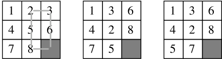
  Figure 2.1: The two configurations to the left can reach each other by the path indicated (the arrows indicate the (clockwise) motion of the empty square). The rightmost configuration cannot be reached since it differs by only one transposition from the middle one.

  Two such configurations can only be obtained from each other if the empty square describes a closed path, and this invariably corresponds to an even number of steps (transpositions) of the empty square. The first two configurations in figure 2.1 can be obtained by such a path. The third configuration (to the right) differs from the middle one in only one transposition. It can therefore not be obtained by a local algorithm. Ergodicity breaking of the present type is very easily fixed, by simply considering a larger class of possible moves.

• The much more vicious ergodicity breaking appears when the algorithm is “formally correct”, but is simply too slow. After a long simulation time, the algorithm may not have visited all the relevant corners of configuration space. The algorithm may be too slow by a constant factor, a factor $N$, or $\exp(N)$ …. Ergodicity breaking of this kind sometimes goes unnoticed for a while, because it may show up clearly only in particular variables, etc. Very often, the system can be solidly installed in some local equilibrium, which does however not correspond to the thermodynamically stable state. It always invalidates the Monte Carlo simulation. There are many examples of this type of ergodicity breaking, e. g. in the study of disordered systems. Notice that the abstract proof that no “trivial” accident happens does not protect you from a “vicious” one.

For Orientation (and knowing that I may add to the confusion) I would want to warn the reader to think that in a benign simulation all the configuration have a reasonable chance to be visited. This is not at all the case, even in small systems. Using the very fast algorithm for the Ising model which I presented in the last chapter, you may for yourself generate energy histograms of, say, the $20\times 20$ Ising model at two slightly different temperatures (above the Curie point). Even for very small differences in temperature, there are many configurations which have no practical chance to ever be generated at one temperature, but which are commonly encountered at another temperature. This is of course the legacy of the Metropolis method where we sample configurations according to their statistical weight $\pi(x)\sim\exp[-\beta E(x)]$. This socalled “Importance Sampling” is the rescue (and the danger) of the Monte Carlo method - but is related only to the equilibrium properties of the process. Ergodicity breaking - a sudden slowdown of the simulation - may be completely unrelated to changes in the equilibrium properties of the system. There are a few models in which this problem is discussed. In my opinion, none is as accessible as the work of ref [7] which concerns a modified Ising model, which undergoes a purely dynamic roughening transition.

We retain that the absolute probability $p(a\rightarrow\ldots\rightarrow b)>0$ can very rarely be evaluated explicitly, and that the formal mathematical analysis is useful only to detect the “trivial” kind of ergodicity violation. Very often, careful data analysis and much physical insight is needed to assure us of the practical correctness of the algorithm.

2.1.1 Dynamics

One is of course very interested in the numerical study of the phenomena associated with very slow dynamics, such as relaxation close to phase transitions, as glasses, spin glasses, etc. We have just seen that these systems are a priori difficult to study with Monte Carlo methods, since the stationary distribution is never reached during the simulation.

It is characteristic of the way things go in Physics that - nonwithstanding these difficulties - there is often no better method to study these systems than to do a …Monte Carlo simulation! In Dynamical Monte Carlo, one is of course bound to a specific Monte Carlo algorithm, which serves as a model for the temporal evolution of the system from one local equilibrium state to another. In these cases, one knows by construction that the Monte Carlo algorithm will drive the system towards the equilibrium, but very often after a time much too large to be relevant for experiment and simulation. So one is interested in studying relaxation of the system from a given initial configuration.

The conceptual difference of the equilibrium Monte Carlo (which was treated in the last chapter) with the dynamical Monte Carlo methods cannot be overemphasized. In the first one, we have an essentially unrestricted choice of the algorithm (expressed by the a priori probability, which was discussed at length), since one is exclusively interested in generating independent configurations $x$ distributed according to $\pi(x)$. In the thermodynamic Monte Carlo, the temporal correlations are just a nuisance. As we turn to dynamical calculations, these correlations become the main object of our curiosity. In dynamical simulations, the a priori probability is of course fixed. Also, if the Monte Carlo algorithm is ergodic both in principle and in practice, the static results will naturally be independent of the algorithm.

You may ask whether there is any direct relationship between the Metropolis dynamics (which serves as our Model), and the true physical time of the experiment, which would be obtained by a numerical integration of the equations of motion, as is done for example in molecular dynamics. There has been a lot of discussion of this point and many simulations have been devoted to an elucidation of this question for, say, the hard sphere liquid. All these studies have confirmed our intuition (as long as we stay with purely local Monte Carlo rules): the difference between the two approaches corresponds to a renormalization of time, as soon as we leave a ballistic regime (times large compared to the mean-free time). The Monte Carlo dynamics is very often simpler to study.

In equilibrium Monte Carlo, theory does not stop with the naive Metropolis algorithm. Likewise, in dynamical simulation there is also room for much algorithmic subtlety. In fact, even though our model for the dynamics is fixed, we are not forced to implement the Metropolis rejections blindly on the computer. Again, it’s the rate of rejections which serves as an important indicator that something more interesting than the naive Metropolis algorithm may be tried. The keyword here are faster than the Clock algorithms which are surprisingly little appreciated, even though they often allow simulations of unprecedented speed.

2.2 Playing dice

As a simple example which is easy to remember, consider the system shown in figure 2.2: a single spin, which can be $S=\pm 1$ in

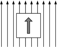
Figure 2.2: Here, we look at the dynamics of a single spin in a magnetic field. We will soon relate it …

a magnetic field $\mathcal{H}$, at finite temperature. The energy of each of the two configurations is

$$E=-\mathcal{H}\;S$$ (2.1)

We consider the Metropolis algorithm of eq. (1.10) to model the dynamical evolution of the system and introduce an explicit time step $\Delta\tau=1$.

$$p(S\rightarrow-S,\Delta\tau)=\Delta\tau\left\{\begin{array}[]{cl}1&(\mbox{if}\;E(-S)<E(S))\\ \exp[-\beta(E(-S)-E(S))]&(\mbox{otherwise})\end{array}\right.$$ (2.2)

To be completely explicit, we write down again how the spin state for the next time step is evaluated in the Metropolis rejection procedure: at each time step $t=1,2,\ldots$ we compute a random number $0<ran<1$ and compare it with the probability $p$ from eq. (2.2):

$$S_{t+1}=\left\{\begin{array}[]{cl}-S_{t}&\mbox{if}\;p(S_{t}\rightarrow-S_{t})>\mbox{ran}\\ S_{t}&\mbox{otherwise}\end{array}\right.$$ (2.3)

This rule assures that, asymptotically, the two configurations are chosen with the Boltzmann distribution. Notice that, whenever we are in the excited “$-$” state of the single spin model, our probability to fall back on the next time step is $1$, which means that the system will flip back to the “$+$” state on the next move. Therefore, the simulation will look as follows:

$$\ldots++++\framebox{- +}+\framebox{- +}++\framebox{- +}++++\framebox{- +}++\framebox{- +}\ldots$$ (2.4)

As the temperature is lowered, the probability to be in the excited state will gradually diminish, and you will spend more and more time computing random numbers in eq. (2.3), but rejecting the move from $S=+1$ to $S=-1$.

At the temperature $\beta=\log(6)/2$, the probability to flip the spin is exactly $1/6$, and the physical problem is then identical to the game of the little boy depicted in figure 2.3. He is playing with

Figure 2.3: …to the game of this little boy. There is a simpler way to simulate the dynamics of a single spin than to throw a die at each time step. The solution is indicated in the lower part: the shaded space corresponds to the probability of obtaining a “flip” on the third throw.

a special die, with $5$ empty faces (corresponding to the rejections $S_{t+1}=S_{t}=1$) and one face with the inscription “flip” ($S_{t+1}=-S_{t}$, $S_{t+2}=-S_{t+1}$). The boy will roll the die over and over again, but of course most of the time the result of the game is negative. As the games goes on, he will expend energy, get tired, etc etc, mostly for nothing. Only very rarely does he encounter the magic face which says “flip”. If you play this game in real life or on the computer, you will soon get utterly tired of all these calculations which result in a rejection, and you may get the idea that there must be a more economical way to arrive at the same result. In fact, you can predict analytically what will be the distribution of time intervals between “flips”. For the little boy, at any given time, there is a probability of $5/6$ that one roll of the die will result in a rejection, and a probability of $(5/6)^{2}$ that two rolls result in successive rejections, etc. The numbers $(5/6)^{l}$ are shown in the lower part of figure 2.3. You can easily convince yourself that the shaded space in the figure corresponds to the probability $(5/6)^{2}-(5/6)^{3}$ to have a flip at exactly the third roll. So, to see how many times you have to wait until obtaining a “flip”, you simply draw a random number ran $0<ran<1$, and check into which box it falls. The box index $l$ is calculated easily:

$$(5/6)^{l+1}<ran<(5/6)^{l}\Rightarrow l=\mbox{Int}\left\{\frac{\log{ran}}{log(5/6)}\right\}.$$ (2.5)

What this means is that there is a very simple program “dice.f”, which you can obtain from my WWW-site, and which has the following characteristics:

• the program has no rejection. For each random number drawn, the program computes a true event: the waiting time for the next flip.

• The program thus is “faster than the clock” in that it is able to predict the state of the boy’s log-table at simulation time t with roughly t/6 operations.

• the output of the accelerated program is completely indistinguishable from the output of the naive Metropolis algorithm.

You see that to determine the temporal evolution of the die-playing game you don’t have to do a proper “simulation”, you can use a far better algorithm.

It is of course possible to generalize the little example from a probability $\lambda=1/6$ to a general value of $\lambda$, and from a single spin to a general statistical mechanics problem with discrete variables. …I hope you will remember the trick next time that you are confronted to a simulation, and the terminal output indicates one rejection after another. So you will remember that the proper rejection method eq. (2.3) is just one possible implementation of the Metropolis algorithm eq. (2.2). The method has been used to study different versions of the Ising model, disordered spins, kinetic growth and many other phenomena. At low temperatures, when the rejection probabilities increase, the benefits of this method can be enormous.

So, you will ask why you have never heard of this trick before. One of the reason for the relative obscurity of the method can already be seen on the one-spin example: In fact you see that the whole method does not actually use the factor $1/6$, which is the probability to do something, but with $5/6=1-1/6$, which is the probability to do nothing. In a general spin model, you can flip each of the $N$ spins. As input to your algorithm computing waiting times, you again need the probability “to do nothing”, which is

$$1-\lambda=1-\sum_{i=1}^{N}[\mbox{probability to flip spin $i$}]$$ (2.6)

If these probabilities all have to be computed anew for each new motion, the move becomes quite expensive (of order $N$). A straightforward implementation therefore has all the chances to be too onerous to be extremely useful. In practice, however, you may encounter enormous simplifications in evaluating $\lambda$ for two reasons:

• you may be able to use symmetries to compute all the probabilities. Since the possible probabilities to flip a spin fall into a finite number $n$ of classes. The first paper on accelerated dynamical Monte Carlo algorithms [6] has coined the name “n-fold way” for this strategy.

• You may be able to simply look up the probabilities, instead of computing them, since you didn’t visit the present configuration for the first time and you took notes [12].

2.3 Accelerated Algorithms for Discrete Systems

We now discuss the main characteristics of the method, as applied to a general spin model with configurations $S_{i}$ made up of $N$ spins $S_{i}=(S_{i,1},\ldots,S_{i,N})$. We denote the configuration obtained from $S_{i}$ by flipping the spin $m$ as $S_{i}^{[m]}$. The system remains in configuration $S_{i}$ during a time $\tau_{i}$, so that the time evolution can be written as

$$S_{1}(\tau_{1})\rightarrow S_{2}(\tau_{2})\ldots\rightarrow S_{i}(\tau_{i})\rightarrow S_{i+1}(\tau_{i+1})\ldots etc$$ (2.7)

The probability of flipping spin $m$ is given by

$$p(S_{i}\rightarrow S_{i}^{[m]},\Delta\tau)=\frac{\Delta\tau}{N}\left\{\begin{array}[]{cl}1&(\mbox{if}\;\;E(S_{i}^{[m]})<E(S_{i}))\\ \exp[-\beta(\Delta E)]&(\mbox{otherwise})\end{array}\right.$$ (2.8)

where the $1/N$ factor expresses the the $1/N$ probability to select the spin $m$. After computing $\lambda=\sum_{i}p(S_{i}\rightarrow S_{i}^{[m]})$, we obtain the waiting time as in eq. (2.5), which gives the exact result for a finite values of $\Delta\tau$. Of course, in the limit $\Delta\tau\rightarrow 0$, the eq. (2.5) simplifies, and we can sample the time to stay in $S_{i}$ directly from an exponential distribution $p(\tau_{i})=\lambda\exp(-\lambda\tau_{i})$ (cf [8] chap. 7.2 for how to generate exponentially distributed random numbers).

If we have then found out that after a time $\tau$ we are going to move from our configuration $S$, where are we going? The answer to this question can be simply understood by looking at figure 2.4:

Figure 2.4: “Pile” of probabilities, which allows us to understand how we decide on the spin to flip. Accelerated algorithms make sense if, usually, $\lambda<<1$.

there we see the “pile” of all the probabilities which were computed. If the waiting time $\tau_{i}$ is obtained from $\lambda_{i}$, we choose the index $[m]$ of the flipped spin with a probability $p(S\rightarrow S^{[m]})$. To do this, you need all the elements to produce the box in figure 2.4 i. e. the probabilities:

$$\begin{array}[]{l}p(S\rightarrow S^{[1]})+p(S\rightarrow S^{[2]})+\ldots p(S\rightarrow S^{[N]})=\lambda\\ \vdots\\ p(S\rightarrow S^{[1]})+p(S\rightarrow S^{[2]})\\ p(S\rightarrow S^{[1]})\\ \end{array}$$ (2.9)

In addition, one needs a second random number ($0<ran<\lambda$) to choose one of the boxes (cf the problem in figure 2.3). The best general algorithm to actually compute $m$ is of course not “visual inspection of a postscript figure”, but what is called “search of an ordered table”. This you find explained in any book on basic algorithms (cf, for example [8], chap. 3.2). Locating the correct box only takes of the order of $\log(N)$ operations. The drawback of the computation is therefore that any move costs an order of $N$ operations, since in a sense we have to go through all the possibilities of doing something before knowing our probability “to do nothing”. This expense is the price to be payed in order to completely eliminate the rejections.

2.4 Implementing Accelerated Algorithms

Once you have understood the basic idea of accelerated algorithms, you may wonder how these methods are implemented, and whether it’s worth the trouble. In cases in which the local energy is the same for any lattice site, you will find out that the probabilities can take on only $n$ different values. In the case of the $2$-dimensional Ising model, there are $10$ classes that the spin can belong to, ranging from up-spin with $4$ neighboring up-spins, up-spin with $3$ neighboring up-spins, to down-spin with $4$ neighboring down-spins. Knowing the repartition into different classes at the initial time, you see that flipping the spin changes the classes of $5$ spins, and can be seen as a change of the number of particles belonging to the different classes. Using a somewhat more intricate bookkeeping, we can therefore compute the value of $\lambda$ in a constant number of operations, and the cost of making a move is reduced to order $O(1)$. You see that the accelerated algorithm has truly solved the problem of small acceptance probabilities which haunts so many simulations at low temperature (for practical details, see refs [6], [15]).

…If you program the method, the impression of bliss may well turn into frustration, for we have overlooked an important point: the system’s dynamics, while without rejections, may still be futile. Consider for concreteness an energy landscape as in figure 2.5,

Figure 2.5: Rugged energy “landscape” which poses problems in a dynamical Monte Carlo simulation at low temperatures. The system will be stuck in one of the local minima, and the dynamics will be futile, i. e. very repetitive.

where any configuration (one of the little dots) is connected to two other configurations. Imagine the system at one of the local minima at some initial time. At the next time step, it will move to one of the neighboring sites, but it will almost certainly fall back right afterwards. At low temperature, the system will take a very long time (and, more importantly, a very large number of operations) before hopping over one of the potential barriers. In these cases, the dynamics is extremely repetitive, futile. If such behavior is foreseeable, it is of course wasteful to recompute the “‘pile of probabilities” eq. (2.9), and even to embark on the involved book-keeping tricks of the n-fold way algorithm. In these cases, it is much more economical to save much of the information about the probabilities, and to look up all the relevant information. An archive can be set up in such a way that, upon making the move $S_{i}\rightarrow S_{i}^{[m]}$ we can quickly decide whether we have seen the new configuration before, and we can immediately look up the “pile of probabilities”. This leads to extremely fast algorithms (for practical details, see [11], [12]). Systems in which this approach can be used contain: flux lines in a disordered superconductor, the NNN Ising model [7] alluded to earlier, disordered systems with a so-called single-step replica symmetry breaking transition, and in general systems with steep local minima. For these systems it is even possible to produce a second-generation algorithm, which not only accepts a move at every timestep, but even a move to a configuration which the system has never seen before. One such algorithm has been proposed in [11], cf also [16].

There are endless possibilities to improve the dynamical algorithms for some systems. Of course, the more powerful a method the less frequently it can be applied. It should be remembered that the above method is only of use if the probability to do nothing is very large, and/or if the dynamics is very repetitive (steep local minimum of energy function in figure 2.5). A large class of systems for which none of these conditions hold are the spin glasses with a socalled continuous replica symmetry breaking transition, as the Sherrington-Kirkpatrick model. In these cases, the ergodicity breaking takes place very “gracefully”, there are very many configurations accessible for any given initial condition. In this case, there seems to be very little room for improvements of the basic method.

2.5 Random Sequential Adsorption

I do not want to leave the reader with the impression that the accelerated algorithms are restricted only to spin models. In fact, intricate rapid methods can be conceived in most cases in which you have many rejections in a dynamical simulation. These rejections simply indicate that the time to “do something” may be much larger than the simulation time step.

The following example, random sequential adsorption, was already mentioned in section 1.1. Imagine a large two-dimensional square on which you deposit one coin per second - but attention: we only put the coin if it does not overlap with any of the coins already deposited. The light-gray coin in the figure 2.6 will immediately be taken away.

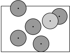
Figure 2.6: Random sequential adsorption: the light coin - which has just been deposited - has to be taken away again.

Random sequential adsorption is a particularly simple dynamical system because of its irreversibility. We are interested in two questions:

• The game will stop at the moment at which it is impossible to deposit a new coin. What is the time after which this “jamming” state is reached and what are its properties?

• We would also like to know the mean density as a function of time for a large number of realizations.

I will give here a rather complete discussion of this problem in six steps, displaying the panoply of refinements which can be unfolded as we come to understand the program. There is a large research literature on the subject, but you will see that you can yourself find an optimal algorithm by simply applying what we have learned in the problem of the rolling die.

2.5.1 Naive Algorithm

You can write a program simulating in a few minutes. You need a table which contains the ($x,y$) positions of the $N(t)$ coins already deposited, and a random number generator which will give the values of $x,y$. If you run the program, you will see that even for modest sizes of the box, it will take quite a long time before it stops. You may say “Well, the program is slow, simply because the physical process of random absorption is slow, there is nothing I can do …”. If that is your reaction, you may gain something from reading on. You will find out that there is a whole cascade of improvement that can be imported into the program. These improvements concern not only the implementation details but also the deposition process itself, which can be simulated faster than in the experiment - especially in the final stages of the deposition. Again, there is a Faster than the Clock algorithm, which deposits (almost) one particle per unit time. These methods have been very little explored in the past.

2.5.2 Underlying Lattice

The first thing you will notice is that the program spends a lot of time computing distances between the proposed point ($x,y$) and the coins which are already deposited. It is evident that you will gain much time by performing only a local search. This is done with a grid, as shown in figure 2.7 and by computing the table of all the particles contained in each of the little squares. As you try to deposit the particle at $(x,y)$, you first

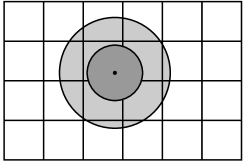
Figure 2.7: One of the basic techniques to orient oneself is introducing a grid. The exclusion area of the coin is also shown.

compute the square which houses the point ($x,y$) and then compute the overlaps with particles contained in neighboring squares. Some bookkeeping is necessarily involved, and varies with the size of the squares adopted. There has been a lot of discussion about how big the little squares have to be taken, and there is no clear-cut answer. Some people prefer a box of size approximately $\sqrt{2}$ times the radius of the spheres. In this case you are sure that at most $1$ sphere per square is present, but the number of boxes which need to be scrutinized is quite large. Others have adopted larger boxes which have the advantage that only the contents of $9$ boxes have to be checked. In any case, one gains an important factor N with respect to the naive implementation.

2.5.3 Stopping criterion

Since we said that we want to play the game up to the bitter end, you may want to find out whether there is at all a possibility to deposit one more coin. The best thing to do is to write a program which will tell you whether the square can host one more point. To do this, you have to apply basic trigonometry to find out whether the whole square is covered with “exclusion disks”, as shown in figure 2.7

2.5.4 Excluding Squares

Try to apply the idea of an exclusion disk to the configuration shown in figure 2.8. Using the idea of the exclusion disk, you will be able to compute the parts of the field on which you can still deposit a new coin. These parts have been designed in dark, we call them

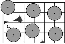
Figure 2.8: Even though there is much empty space, we can only deposit further coins on three “stars” (belonging to $4$ of the $24$ squares making up the field).

“stars” for obvious reasons. You can see that, at the present moment, there are only $4$ of the $24$ grid-squares which can take on a new point. Before starting to compute distances with coins in adjacent squares, it may be a good idea to check at all whether it is possible to deposit a box on the point. You will quickly realize that we are confronted with exactly the same problem as the boy in figure 2.3: only one out of six grid-squares has a non-zero chance to accept a new coin. The time for the next hit of one of the useful squares can be obtained with a one-sides die, or, equivalently, sampled from eq. (2.5). So, you can write a faster (intermediate) program, by determining which of the boxes can still hold a coin. This probability then gives the probability “to do nothing”, which is used in eq. (2.5) to sample the time after which a new deposition is attempted. Are you tempted to write such a program? You simply need a subroutine able to determine whether there is still free space in a square. With such a subroutine you are able to exclude squares from the consideration. The ratio of excluded squares to the total number of squares then gives the probability $1-\lambda$ to do nothing, which is what you need for the faster-than-the-clock algorithm of section 2.2.

2.5.5 The Ultimate Algorithm

Cutting up the field into little squares allows us a second time to make the program run faster by a factor $N$, where $N$ is the number of little squares. Not only can we use the squares to simplify the calculation of overlaps, but to exclude large portions of the field from the search.

Unfortunately, you will quickly find out that the program still has a very large rejection probability …just look at the square denoted by an a in figure 2.3: roughly $2\%$ of the square’s surface can only accept a new coin. So, you will attempt many depositions in vain before being able to do something reasonable. One idea to go farther consists in going to smaller and smaller squares. This has been implemented in the literature [10]. What one really wants to do, however, is to exploit the exact analogy between the area of the stars, and the probabilities in eq. (2.9). If we know the location and the area of the stars, we are able to implement one of the rejection-free algorithms. Computing the area of a “star” is a simple trigonometric exercise. Having such a subroutine at our disposal allows us to envision the ultimate program for random sequential adsorption.

• Initially, you do the naive algorithm for a while

• Then you do a first cut-up into stars. The total relative area of the field not covered by stars corresponds to the factor $\lambda$, and you will sample the the star for the next deposition exactly as in eq. (2.9). Then you randomly deposit ($x,y$) into the star chosen, and update the book keeping.

2.5.6 How to sample a Random Point in a Star

So, finally, this breath-taking, practical discussion brings us to ponder a philosophical question: how to sample loci in a star. In fact, how do we do that?. For my part, I have given up looking for a rejection-free method to solve this problem - I simply sample a larger square, as in figure 2.9, and then use the good old rejection method. But perhaps you know how to do this?

Figure 2.9: The ultimate algorithm for random sequential adsorption needs a program to calculate the area of a star (straightforward), and a method to sample a random point within it. Can you sample random points within the star without rejections?

2.5.7 Literature, extensions

Of course, the example of the random adsorption was only given to stimulate you to think about better algorithms for Your current Monte Carlo problem, and how it may be possible in your own research problem to get away from a blind use of algorithms. If you want to know more about random deposition, notice that there is a vast research literature, and an algorithm has been presented in [10]. Notice that in our algorithm it was very important for the spheres to be monodisperse, ie for them all to have the same diameter. What can be done in the contrary case? Are there accelerated algorithms for spheres with some distribution of diameters (from $d_{min}$ to $d_{max}$) (easy), and what would be an optimal algorithm for deposition of objects with additional degrees of freedom? The problem is of some interest in the case of ellipses. Evidently, from a numerical point of view, you will end up with a three-dimensional “star” in which you have to sample ($x,y,\theta$), where $\theta$ gives the orientation of the ellipse to be deposited. You may be inspired to think about such a simulation. Remember that it is not important to compute the $3-d$ star exactly, just as, in the last chapter, it was without real importance that the a priori probability $\mathcal{A}(x)$ could be made exactly to $\pi(x)$.

Bibliography

- [1] N. Metropolis, A. W. Rosenbluth, M. N. Rosenbluth, A. H. Teller, E. Teller, J. chem. Phys 21 1087 (1953)
- [2] Monte Carlo Methods in Statistical Physics, edited by K. Binder, 2nd ed. (Springer Verlag, Berlin, 1986)
- [3] S. Caracciolo, A. Pelissetto, A. D. Sokal, Phys. Rev. Lett 72 179 (1994)
- [4] R. H. Swendsen and J.-S. Wang Phys. Rev. Lett. 63, 86 (1987)
- [5] U. Wolff Phys. Rev. Lett. 62, 361 (1989)
- [6] A. B. Bortz, M. H. Kalos, J. L. Lebowitz; J. Comput. Phys. 17, 10 (1975) cf also : K. Binder in [2] sect 1.3.1
- [7] J. D. Shore, M. Holzer, J. P. Sethna; Phys Rev. B 46 11376 (1992)
- [8] W. H. Press, S. A. Teukolsky, W. T. Vetterling, B. P. Flannery, Numerical Recipes, 2nd edition, Cambridge University Press (1992).
- [9] E. L. Pollock, D. M. Ceperley Phys. Rev. B 30, 2555 (1984), 36 8343 (1987); D. M. Ceperley Rev. Mod. Phys 67, 1601 (1995)
- [10] J-S Wang Int. J. Mod. Phys C 5, 707 (1994)
- [11] W. Krauth, O. Pluchery J. Phys. A: Math Gen 27, L715 (1994)
- [12] W. Krauth, M. Mézard Z. Phys. B 97 127 (1995)
- [13] A. E. Ferdinand and M. E. Fisher Phys. Rev. 185 185 (1969)
- [14] J. Lee, K. J. Strandburg Phys Rev. B 46 11190 (1992)
- [15] M. A. Novotny Computers in Physics 9 46 (1995)
- [16] M. A. Novotny Phys. Rev. Lett. 74 1 (1995) Erratum: 75 1424 (1995)