Boundary conformal field theory approach to the critical two-dimensional Ising model with a defect line

Abstract

We study the critical two-dimensional Ising model with a defect line (altered bond strength along a line) in the continuum limit. By folding the system at the defect line, the problem is mapped to a special case of the critical Ashkin-Teller model, the continuum limit of which is the $Z_{2}$ orbifold of the free boson, with a boundary. Possible boundary states on the $Z_{2}$ orbifold theory are explored, and a special case is applied to the Ising defect problem. We find the complete spectrum of boundary operators, exact two-point correlation functions and the universal term in the free energy of the defect line for arbitrary strength of the defect. We also find a new universality class of defect lines. It is conjectured that we have found all the possible universality classes of defect lines in the Ising model. Relative stabilities among the defect universality classes are discussed.

1 Introduction

Boundary (surface) critical phenomena [1] in two-dimensional systems have attracted a lot of interest. Even if the bulk system is a free system, the presence of the boundary makes the problem non-trivial. Boundary conformal field theory [2] is a powerful tool to solve these problems. Its applications to quantum impurity problems are also discussed [3]. A variation of the problem has a defect line inside a two-dimensional system. This kind of problem can still be mapped to a system with boundary, by folding the system at the defect line [4].

The two-dimensional Ising model, which was solved 50 years ago by Onsager [5], is still useful to test new techniques and ideas in statistical mechanics. In this paper, we apply boundary conformal field theory to the two-dimensional Ising model with a defect line. This problem has been studied by several authors. Bariev [6] found a continuously varying “surface” critical exponent. McCoy and Perk [7] and Kadanoff [8] discussed the correlation functions along the defect line. Brown [9] discussed several properties of this model. In particular, he calculated two-point spin correlation function for general locations, in first-order perturbation of the defect strength. Several other studies are focused on the finite-size scaling of the transfer-matrix spectrum on a cylinder. Cabrera and Julien [14] calculated the spectrum numerically. Following the application of conformal invariance by Turban [10] (see also Ref. [11]), Henkel et. al. [12, 13] studied the spectrum of the quantum version by various methods and discussed the spectrum in terms of Virasoro and Kac-Moody algebras. Exact formulae for the spectrum on the square lattice with general anisotropy are given by Abraham et. al. [15]. Grimm [16] also examined generalizations of the defect line. Recently, an $S$-matrix approach to the problem was also presented by Delfino et. al. [17].

In this paper, we study the continuum limit at the critical point. To relate this problem to boundary conformal field theory, we “fold” the system into a $c=1$ conformal field theory with a boundary. Using the exact partition function, we identify the boundary states in terms of $c=1$ conformal field theory. Folding the Ising model gives two decoupled Ising models in the bulk, which is a special case of the Ashkin-Teller model. The critical theory of the Ashkin-Teller model is a $c=1$ conformal field theory: the $Z_{2}$ orbifold of a free boson. We explore the possible boundary states of the orbifold theory and apply a special case to the Ising defect problem.

Identification of the boundary states enables us to give the complete spectrum of “surface” critical exponents for general strength of the defect. Cardy and Lewellen [19] showed that the boundary correlation functions can be determined from the boundary state and the Operator Product Expansion (OPE) in the bulk. We employ this idea to calculate the exact two-point spin correlation function, using Zamolodchikov’s solution [20] for $c=1$ conformal blocks of spin operators. We also calculate certain four-point correlation functions, as well as some correlation function near the end of the defect line. A universal term in the free energy with a finite length defect is also given. Moreover, we find a new one-parameter universality class of defect lines in terms of boundary conformal field theory. We calculate two-point spin correlation functions and then identify a corresponding defect in the quantum lattice model. Finally, the relative stability of the defect universality classes is discussed, and a conjecture is made regarding the complete set of defect universality classes.

The organization of the paper is as follows. In Section 2, we derive the partition function of the model in the critical continuum limit. We use the result to identify the boundary condition in terms of Ashkin-Teller model in Section 3. The possible boundary states on the $Z_{2}$ orbifold theory is explored in Section 4, and further applied to the present problem. In Section 5, we calculate two-point correlation functions and other universal quantities for arbitrary strength of the defect. A new one-parameter family of defect lines is studied in Section 6. In Section 7, we discuss the relative stability and renormalization-group flow among the defect universality classes. We give a summary and some discussion in Section 9.

A brief description of the present work has appeared in [18].

2 Partition function at the critical point

Here we derive the partition function of the Ising model with a defect line, in the continuum limit. While Henkel et. al. [12, 13] have found the result in the $\tau$-continuum limit (quantum Ising chain), here we derive the partition function for the square lattice Ising model with an arbitrary anisotropy, taking the continuum limit of the analysis by Abraham et. al. [15]. Apart from the trivial non-universal parts, the result is independent of the anisotropy, under an appropriate rescaling. It agrees with that of Henkel et. al. which corresponds to the extremely anisotropic limit. This is a manifestation of the universality in the Ising model in the presence of a defect line.

We consider a square-lattice Ising model with the lattice constant $a$. The Ising model on a cylinder with a defect line is defined by the classical Hamiltonian:

$${\cal E}=-\sum_{i=1,M-1}\sum_{j=1,N}[J_{1}\sigma_{i,j}\sigma_{i,j+1}+J_{2}\sigma_{i,j}\sigma_{i+1,j}]-\sum_{j=1,N}[J_{1}\sigma_{M,j}\sigma_{M,j+1}+\tilde{J}\sigma_{M,j}\sigma_{1,j}].$$ (1)

The altered link (defect) is placed between $i=M$ and $i=1$. We denote the defect strength by $b=\tilde{J}/J_{2}$. This model reduces to the periodic boundary condition, the free boundary condition and the antiperiodic boundary condition, respectively for $b=1,0,-1$. We also introduce $K_{1},K_{2}$ and $K^{*}_{1}$ by

$$K_{1}=J_{1}/kT,K_{2}=J_{1}/kT$$ (2)

$$\sinh{K^{*}_{1}}\sinh{K_{1}}=1.$$ (3)

Let us refer to the direction parallel to the defect line as horizontal. For periodic or antiperiodic boundary condition the transfer matrix can be mapped to a free-fermion Hamiltonian [21] by the Jordan-Wigner transformation. However, it is not straightforward for general $b$ because the system lacks translation invariance in the $i$ (vertical) direction and a simple Fourier transformation is not useful. Nevertheless, Abraham, Ko and Svrakic [15] obtained the spectrum of the transfer matrix in the $j$ (horizontal) direction using a spinor approach. We start from their result and apply it to the critical case.

According to their result, the transfer matrix $V$ can be simply expressed by fermion operators, but the Hilbert space is divided into two sectors:

$$V=P_{+}V_{+}+P_{-}V_{-}.$$ (4)

Here $P_{+}$ ($P_{-}$) is the projection operator onto the even (odd) fermion-number sector. However, one must be careful about the definition of the “even” and “odd” sectors. (See below.) The transfer matrices in the two sectors are given by

$$V_{\pm}=\exp{[-\sum_{j=1}^{M}\gamma(ak^{\pm}_{j})(c^{\dagger}_{j}c_{j}-1/2)]}.$$ (5)

The “single-fermion energy” $\gamma$ is given by the Onsager dispersion function

$$\cosh{\gamma(p)}\equiv\cosh{2K^{*}_{1}}\cosh{2K_{2}}-\sinh{2K^{*}_{1}}\sinh{2K_{2}}\cos{p}$$ (6)

and the quantization condition of the wave number $0<k<\pi/a$

$$e^{iMak^{\pm}} = \zeta e^{i\alpha(ak^{\pm},\mp\zeta b)}$$ (7)

$$\tan{\frac{\alpha(p,x)}{2}} \equiv \frac{\sinh{[(1-x)K_{2}]}}{\sinh{[(1+x)K_{2}]}}\tan{\frac{\delta^{*}(p)}{2}}$$ (8)

where $\pm$ in the first equation corresponds to $V_{\pm}$, $a$ is the lattice constant, $\zeta=+1$ or $-1$ which is independent of $V_{\pm}$. $\delta^{*}$ is defined as

$$\sinh{\gamma(p)}\cos{\delta^{*}(p)}=\sinh{2K_{2}}\cosh{2K_{1}^{*}}-\cosh{2K_{2}}\sinh{2K_{1}^{*}}\cos{p}.$$ (9)

Let us discuss the critical point where $K_{2}=K^{*}_{1}$ but $b$ still remains as a free parameter. In order to discuss the universal behavior at large distances, we take the continuum limit $a\rightarrow 0$ (or equivalently consider the scaling limit where the length scale is much larger than the lattice constant), keeping the circumference of the cylinder $L=Ma$ constant.

Then only the low-energy limit of the dispersion relation is relevant in the discussion. It is given by

$$\gamma(k)=v|k|,$$ (10)

where $v$ is a constant (spin wave velocity). In the following, we rescale the horizontal (“imaginary time”) direction so that $v=1$. The transfer matrix can be described by a Hamiltonian in the continuum limit. The Hamiltonians for fermion number even/odd sector are given by

$$H_{\pm}=\sum_{j}|k^{\pm}_{j}|(c^{\dagger}_{j}c_{j}-1/2).$$ (11)

In this limit, $\delta^{*}(k)=\pi/2$ independent of $k$ and the quantization condition (8) is much simplified. Furthermore, we can choose freely the sign of $k$ in the discussion of the energy, because the dispersion function is an even function of $k$. Thus the quantization condition in the continuum limit is written as

$$k^{\pm}=\frac{\alpha(\mp b)}{2\pi}+\frac{2\pi}{L}n$$ (12)

where $n$ is an arbitrary integer and $\alpha$ is now independent of $k$:

$$\tan{\frac{\alpha(x)}{2}}=\frac{\sinh{[(1-x)K_{2}]}}{\sinh{[(1+x)K_{2}]}}.$$ (13)

From this equation, we see that $\alpha(x)$ satisfies

$$\alpha(x)+\alpha(-x)=\pi.$$ (14)

$\alpha(x)$ takes the values $\pi$, $\pi/2$ and $0$ respectively for $x=-1$,$0$ and $1$. When $x\rightarrow\pm\infty$, $\alpha$ is given by

$$\tan{\frac{\alpha(\pm\infty)}{2}}=-e^{\mp 2K_{2}}.$$ (15)

Thus $\pi<\alpha(-\infty)<3\pi/2$ and $-\pi/2<\alpha(\infty)<0$. We note that, in the $K_{2}\rightarrow 0$ limit with the $x\rightarrow\pm\infty$ limit, $\alpha$ approaches the limiting values $\alpha(-\infty)=3\pi/2$ and $\alpha(\infty)=-\pi/2$. The $K_{2}\rightarrow 0$ limit corresponds to the anisotropic limit where the horizontal link becomes very strong. (It should be remembered that we stay at the critical point where $K_{2}=K_{1}^{*}$.) Regarding the horizontal direction as imaginary time, this is the so-called $\tau$-continuum limit [22] of the Ising model. In this limit, the system is equivalent to the one-dimensional quantum Ising model in a transverse field. The quantum Hamiltonian is given by

$$H=-\sum_{n=-\infty}^{\infty}\hat{\sigma}^{x}(n)-\sum_{n\neq 0}\hat{\sigma}^{z}(n-1)\hat{\sigma}^{z}(n)-b\hat{\sigma}^{z}(-1)\hat{\sigma}^{z}(0),$$ (16)

where $\hat{\sigma}^{x,z}(n)$ is a Pauli spin operator at site $n$. This model is the critical transverse Ising model with a defective link between $n=-1$ and $0$.

In eq. (11), we arrived at a rather simple description of the transfer matrix for generalized boundary condition with parameter $b$. Namely, it is always a free fermion Hamiltonian and the dispersion relation (10) is independent of $b$. The only effect of the boundary condition is the “phase shift” $\alpha$ of the wavenumber as in (12). This phase shift is different in even- and odd- fermion number sectors.

We note that the parity of the fermion number is a subtle problem. Exchanging a fermion annihilation operator $c_{k}$ and the corresponding creation operator $c^{\dagger}_{k}$ preserves all the fermion anticommutation relations. However, this procedure flips the fermion number parity operator defined by $(-1)^{F}=(-1)^{\sum_{j}c^{\dagger}_{j}c_{j}}$. Thus the fermion parity operator depends on the definition of the fermion creation/annihilation operators. We fix the fermion operators so that all particles have non-negative energy and the Hamiltonian takes the form of eq. (11). For $\alpha>0$, the two sectors of Hilbert space in (4) actually corresponds to the even/odd fermion number in the above definition:

$$P_{+}=\frac{1+(-1)^{F}}{2},\hfill P_{-}=\frac{1-(-1)^{F}}{2}.$$ (17)

When $\alpha$ changes sign, one of the quantized wavevectors passes through $k=0$. The energy of the corresponding fermion seems to change non-analytically as $|k|$. However, this should be understood as the fermion energy depending on on the parameter linearly but the annihilation/creation operators being exchanged when the single fermion energy becomes negative. Hence the fermion number parity should be flipped when $\alpha$ becomes negative (as long as we keep the above definition of the fermion operators.)

Figure 1: The Ising model the defect line on a cylinder. The defect line is parallel to the cylinder axis.

Let us consider the partition function of the Ising model on a cylinder with circumference $L$ and length $\beta$ (a macroscopic length scale), as shown in Fig. 1. We apply the periodic boundary condition in the $\beta$ direction. The partition function is given by

$$Z={\rm Tr}\exp{(-\beta H)}$$ (18)

where $H=P_{+}H_{+}+P_{-}H_{-}$ is the total Hamiltonian.

First we consider the $-1\leq b\leq 1$ case. Here $\alpha(\pm b)\geq 0$ and thus the assignment (17) is valid. In the following we denote $\alpha(b)$ by simply $\alpha$: $0\leq\alpha\leq\pi$ for $-1\leq b\leq 1$. In the odd ($(-1)^{F}=-1$) sector, the fermion one-particle energies are given by $\epsilon_{n}=|(\alpha+2\pi n)/L|$. The ground state is the fermionic vacuum $|\mbox{vac}\rangle$ which satisfies $c_{k}|\mbox{vac}\rangle=0$. The vacuum still has “zero-point energy”

$$E_{\rm vac}=-\frac{1}{2}\sum_{n}\epsilon_{n}$$ (19)

according to eq. (11). While this quantity apparently diverges (but of course is cut off by the lattice) in the continuum limit, we can extract the universal “Casimir energy” in the odd sector as

$$E^{-}_{\rm vac}=CL+A+\frac{1}{L}\left(\frac{\pi}{6}+\frac{\alpha^{2}}{4\pi}-\frac{\alpha}{2}\right)$$ (20)

where $C$ is a non-universal energy density, which is the order of inverse square of the lattice constant. The second term is a non-universal shift of the ground-state energy due to the defect. (“surface energy”). The last term is the universal Casimir energy.

For even sector, we can simply replace $\alpha$ by $\pi-\alpha$ to obtain

$$E^{+}_{\rm vac}=CL+A+\frac{1}{L}\left(-\frac{\pi}{12}+\frac{\alpha^{2}}{4\pi}\right).$$ (21)

Since there must be at least one fermion in the odd sector, the ground state energy in the odd sector is given by

$$E^{-}_{g}=E^{-}_{\rm vac}+\frac{\pi-\alpha}{L}$$ (22)

The ground state energy in the even sector is simply (21) and is lower than $E^{-}_{g}$. Thus eq. (21) also gives the ground-state energy of the present system. It reduces to the known value for periodic ($\alpha=0$), antiperiodic ($\alpha=\pi$) and free ($\alpha=\pi/2$) cases [29].

In the following we ignore the non-universal part and set $L=1$ for simplicity. (The $L$ dependence can be recovered by simply replacing $\beta\rightarrow\beta/L$.) The partition function in the odd sector is given by

$$Z_{\rm odd}=e^{-\beta E_{\rm vac}}\sum_{\{n_{k}=0,1\}}P_{-}e^{-\beta\sum_{k}\epsilon_{k}n_{k}}$$ (23)

Using

$$P_{-}=\frac{1-(-1)^{F}}{2}=\frac{1-(-1)^{\sum_{k}n_{k}}}{2},$$ (24)

we obtain the infinite product representation of the elliptic theta functions as

$$Z_{\rm odd}=\frac{e^{-\alpha^{2}\beta/4\pi}}{2}\left[\frac{\vartheta_{2}(w,q)}{\eta(q)}+i\frac{\vartheta_{1}(w,q)}{\eta(q)}\right],$$ (25)

where the parameters is given by

$$q=e^{-2\pi\beta},\hfill w=e^{-\alpha\beta}.$$ (26)

In this paper we use the elliptic theta functions and Dedekind eta function

$$\vartheta_{1}(w,q) = i\sum_{n=-\infty}^{\infty}(-1)^{n}q^{\frac{1}{2}(n-\frac{1}{2})^{2}}w^{n-\frac{1}{2}}$$ (27)

$$\vartheta_{2}(w,q) = \sum_{n=-\infty}^{\infty}q^{\frac{1}{2}(n-\frac{1}{2})^{2}}w^{n-\frac{1}{2}}$$ (28)

$$\vartheta_{3}(w,q) = \sum_{n=-\infty}^{\infty}q^{\frac{1}{2}n^{2}}w^{n}$$ (29)

$$\vartheta_{4}(w,q) = \sum_{n=-\infty}^{\infty}(-1)^{n}q^{\frac{1}{2}n^{2}}w^{n}$$ (30)

$$\eta(q) = q^{1/24}\prod_{n=1}^{\infty}(1-q^{n}).$$ (31)

Theta functions with a single argument $\vartheta_{j}(q)$ should be understood as $\vartheta_{j}(w=1,q)$ (“theta constants”).

For the even sector we make a similar calculation and obtain

$$Z_{\rm even}=\frac{e^{-\alpha^{2}\beta/4\pi}}{2}\left[\frac{\vartheta_{3}(w,q)}{\eta(q)}+\frac{\vartheta_{4}(w,q)}{\eta(q)}\right].$$ (32)

Thus the total partition function $Z=Z_{\rm even}+Z_{\rm odd}$ is given by

$$Z_{\rm Ising}=\frac{e^{-\alpha^{2}\beta/4\pi}}{2}\left[\frac{\vartheta_{3}(w,q)}{\eta(q)}+\frac{\vartheta_{4}(w,q)}{\eta(q)}+\frac{\vartheta_{2}(w,q)}{\eta(q)}+i\frac{\vartheta_{1}(w,q)}{\eta(q)}\right],$$ (33)

with the parameters as in eq. (26).

For $|b|>1$, we must flip the fermion parity in the sector with negative phase shift $\alpha$. However, as a result of the calculation, we found that the above equation (33) is still valid in this case. Thus the partition function of the critical Ising model on the cylinder is given by eq. (33) for the entire range $-\infty<b<\infty$. Our result agrees with that by Henkel et. al. [12, 13], which is obtained in $\tau$-continuum limit.

3 Identification of the boundary state by folding

Figure 2: The folding of the Ising model on a cylinder to a $c=1$ theory on a strip. We fold at the defect line and also at the line on the opposite side. These lines correspond to the boundary in the folded system.

In order to apply boundary conformal field theory to the present problem, we fold the system so that the defect line becomes the boundary of the system [4]. The cylinder of circumference $1$ is folded to a strip of width $1/2$, as shown in Fig. 2. In addition to the boundary which corresponds to the defect line, we have another boundary on the opposite side. The two boundaries are identical when there is no defect line, or equivalently when the periodic boundary condition is imposed on the Ising model ($b=1$). As a result of the folding, the degrees of freedom in the bulk are doubled. There are two different kinds of spin operators at each point, corresponding to the locations before the folding. We will call them two different layers of spins. Because of the doubling, we must consider a $c=1$ conformal field theory, rather than $c=1/2$. Known $c=1$ conformal field theories are described by a free boson or its orbifold.

Actually, a useful trick to study the Ising model on a plane is to regard two independent Ising models as a free boson theory [23, 24]. Let us denote the spins in each layer as $\sigma_{1}$ and $\sigma_{2}$. The product $\sigma_{1}\sigma_{2}$ of the spin operators in each layer (at the same point) can be expressed as a simple bosonic operator $\cos{\varphi}$ where $\varphi$ is the free boson field. Since the two Ising models are independent, correlation functions of this composite operator is always the square of the spin correlation in a single layer. Thus we can calculate spin correlation functions of the Ising model in terms of the free boson. In the present problem, the two Ising layers are coupled at the boundary though they are independent in the bulk. This makes the problem more difficult.

The two-dimensional Ashkin-Teller model [25] is defined by the classical Hamiltonian

$${\cal E}=\sum_{\langle xy\rangle}\left\{K[\sigma_{1}(x)\sigma_{1}(y)+\sigma_{2}(x)\sigma_{2}(y)]+L\sigma_{1}(x)\sigma_{1}(y)\sigma_{2}(x)\sigma_{2}(y)\right\},$$ (34)

where $\langle x,y\rangle$ runs over all nearest neighbor pairs on the square lattice. The doubled independent Ising model can be regarded as a decoupling point $L=0$ of the Ashkin-Teller model. Of course this is usually an unnecessary complication when one focuses on the Ising model. However, in the present problem it seems necessary to consider the doubled Ising model as a special case of the Ashkin-Teller model, This will become manifest in Sec. 5.2, where two-spin correlation functions are discussed.

The critical Ashkin-Teller model is identified with a $c=1$ conformal field theory. Precisely speaking, it is not a simple free boson but the $Z_{2}$ orbifold of the free boson. (For a review, see Ref. [26].) We take the normalization of the free boson field so that the Lagrangian is given by

$${\cal L}=\frac{1}{2\pi}(\partial_{\mu}\varphi)^{2}.$$ (35)

The orbifold theory depends on a continuous parameter: the compactification radius $r$ of the free boson (i.e. we make the identification $\varphi\sim\varphi+2\pi r$). The decoupling point (doubled Ising model), which is relevant in our defect problem, corresponds to $r=1$. The boundary condition (or the boundary state, see below) in the present problem can be identified in two (presumably equivalent) ways: in terms of Ashkin-Teller boundary states and in terms of the orbifold free boson. We first describe the former identification, which will be useful in the calculation of the spin correlation function. We will discuss the orbifold boundary state in the next section.

A boundary of the system is described by a boundary state, if we exchange space and time so that the “(imaginary) time” is orthogonal to the boundary. In particular, when the boundary is conformally invariant, the boundary state $|B\rangle$ must satisfy the condition

$$(L_{n}^{(P)}-\bar{L}_{-n}^{(P)})|B\rangle=0,$$ (36)

where $L^{(P)}$ and $\bar{L}^{(P)}$ are the bulk Virasoro generators [27, 28]. A solution to this equation is given by the Ishibashi state

$$|\Delta\rangle\rangle=\sum_{N}|\Delta,N\rangle\otimes|\overline{\Delta,N}\rangle$$ (37)

where $|\Delta,N\rangle$ is a normalized $N$-th descendant of the primary field of weight $\Delta$, and the summation is over all descendants. In this paper, $|\Delta\rangle\rangle$ denotes the Ishibashi state constructed from the primary state with the weight $\Delta$. A linear combination of Ishibashi states also satisfy conformal invariance. In general, the boundary state consists of several Ishibashi states. The corresponding primary weights are included in bulk operator contents. While there are bulk operator with spin, only the spinless primaries ($\Delta=\bar{\Delta}$) are relevant in the boundary state, as is seen from the structure of the Ishibashi states.

The partition function and the operator content of the critical Ashkin-Teller model is studied by Yang [30]. We summarize the spinless primaries at the decoupling point (doubled Ising model) in Table 1. Hereafter we will denote the critical Ashkin-Teller model at the decoupling point simply as “Ashkin-Teller model”.

$\Delta=\bar{\Delta}$	Multiplicity	Degeneracy	Identification
$n^{2}$	1	[degenerate ]	$I_{1}\cdot I_{2}$ ($n=0$); $\epsilon_{1}\cdot\epsilon_{2}$ ($n=1$)
$\frac{(n+1)^{2}}{2}$	2	[non-degenerate ]	$\epsilon_{1}\cdot I_{2},I_{1}\cdot\epsilon_{2}$ ($n=0$)
$\frac{(2n+1)^{2}}{8}$	1	[non-degenerate ]	$\sigma_{1}\cdot\sigma_{2}$ ($n=0$)
$\frac{(2n+1)^{2}}{16}$	2	[non-degenerate ]	$\sigma_{1}\cdot I_{2},I_{1}\cdot\sigma_{2}$ ($n=0$)

Table 1: The spinless primary operators in the critical Ashkin-Teller model (at the decoupling point). $n=0,1,2,\ldots$ and the “degeneracy” means the degeneracy in terms of the $c=1$ Virasoro representation (not the multiplicity of the operators).

A primary state $|I\rangle$ of the Ising model satisfies the condition

$$L_{n}^{\rm Ising}|I\rangle=0\;\;\;\;(n>0)$$ (38)

where $L_{n}^{\rm Ising}$ is a Virasoro generator of the Ising model. A primary state of the Ashkin-Teller model is defined by the condition

$$(L_{n}^{\rm Ising1}+L_{n}^{\rm Ising2})|AT\rangle=0\;\;\;\;(n>0)$$ (39)

Thus a tensor product of two Ising primaries is a primary (or a sum of primaries) of the Ashkin-Teller model, but the reverse is not always true. In fact, there is an infinite number of primaries in the Ashkin-Teller model, while only three primaries are present in the Ising model: the identity operator $I$, the energy density $\epsilon$ and the spin operator $\sigma$. For example, the second set of the above spinless primaries ($\Delta=\bar{\Delta}=(n+1)^{2}/2$) is identified as follows. There are two primaries for each dimension. For $n$ even ($\Delta=\bar{\Delta}=(2m+1)^{2}/2$), the two Ashkin-Teller primaries are $\epsilon_{1}\cdot I_{2}$ and $I_{1}\cdot\epsilon_{2}$ ($n=0$) or corresponding Ising descendants ($n\geq 1$). We will distinguish them as $|\frac{(2m+1)^{2}}{2},1\rangle\rangle$ and $|\frac{(2m+1)^{2}}{2},2\rangle\rangle$. For $n$ odd ($\Delta=\bar{\Delta}=2m^{2}$), the two primaries are Ising descendants of $I_{1}\cdot I_{2}$ and $\epsilon_{1}\cdot\epsilon_{2}$. We will distinguish corresponding Ishibashi states as $|2m^{2},II\rangle\rangle\equiv|2m^{2},1\rangle\rangle$ and $|2m^{2},\epsilon\epsilon\rangle\rangle\equiv|2m^{2},2\rangle\rangle$.

Let us write the tensor product of the Ising Ishibashi states as Ashkin-Teller Ishibashi states. For example, we consider the Ising Ishibashi state $|I\rangle\rangle$ of the identity operator $I$. (Note that it is not a physically allowed boundary state of the Ising model without superposition with other Ishibashi states [28].) The partition function on a strip of width $1/2$ and length $\beta$ with two boundaries specified by the Ishibashi state $|I\rangle\rangle$ is given by the $c=1/2$ Virasoro character [29]

$$\chi_{I}(\tilde{q})=\frac{1}{2\eta(\tilde{q})}[\vartheta_{3}(\tilde{q})+\vartheta_{4}(\tilde{q})]$$ (40)

where $\tilde{q}$ is defined as

$$\tilde{q}=e^{-2\pi/\beta}.$$ (41)

Let us consider the Ashkin-Teller boundary state defined by the tensor product of the Ising Ishibashi state $|I_{1}\rangle\rangle\otimes|I_{2}\rangle\rangle$. The partition function of the Ashkin-Teller model on the strip with the corresponding boundary condition on both boundaries is given by the square of eq. (40). Regarding the Ashkin-Teller model as a $c=1$ conformal field theory, it should be possible to express it in terms of $c=1$ Virasoro characters. The $c=1$ Virasoro characters [31] for the primary weight $h$ are given by

$$\chi_{h}(q)=\frac{q^{h}}{\eta(q)},$$ (42)

if $h\neq n^{2}/4$. When $h=n^{2}/4$, the representation is degenerate and the character $\chi_{h}$ is rather given by

$$\chi_{h}(q)=\frac{q^{n^{2}/4}-q^{(n+2)^{2}/4}}{\eta(q)}.$$ (43)

The partition function on the strip is expressed as

$$\chi_{I}(\tilde{q})^{2}=\sum_{n=1}^{\infty}\chi_{2n^{2}}(\tilde{q})+\sum_{n=0}^{\infty}\chi_{(2n)^{2}}(\tilde{q}).$$ (44)

Thus the boundary state is identified in terms of Ashkin-Teller Ishibashi states as

$$|I_{1}\rangle\rangle\otimes|I_{2}\rangle\rangle=\sum_{n=1}^{\infty}|2n^{2},II\rangle\rangle+\sum_{n=1}^{\infty}|(2n)^{2}\rangle\rangle.$$ (45)

Similarly, we identify other tensor products as follows.

$$|\epsilon_{1}\rangle\rangle\otimes|\epsilon_{2}\rangle\rangle = \sum_{n=1}^{\infty}|2n^{2},\epsilon\epsilon\rangle\rangle+\sum_{n=0}^{\infty}|(2n+1)^{2}\rangle\rangle$$ (46)

$$|\sigma_{1}\rangle\rangle\otimes|\sigma_{2}\rangle\rangle = \sum_{n=0}^{\infty}|\frac{(2n+1)^{2}}{8}\rangle\rangle$$ (47)

$$|I_{1}\rangle\rangle\otimes|\epsilon_{2}\rangle\rangle = \sum_{n=0}^{\infty}|\frac{(2n+1)^{2}}{2},2\rangle\rangle$$ (48)

$$|\epsilon_{1}\rangle\rangle\otimes|I_{2}\rangle\rangle = \sum_{n=0}^{\infty}|\frac{(2n+1)^{2}}{2},1\rangle\rangle$$ (49)

$$|I_{1}\rangle\rangle\otimes|\sigma_{2}\rangle\rangle = \sum_{n\equiv 0,3({\rm mod}4)}|\frac{(2n+1)^{2}}{16},2\rangle\rangle$$ (50)

$$|\sigma_{1}\rangle\rangle\otimes|I_{2}\rangle\rangle = \sum_{n\equiv 0,3({\rm mod}4)}|\frac{(2n+1)^{2}}{16},1\rangle\rangle$$ (51)

$$|\epsilon_{1}\rangle\rangle\otimes|\sigma_{2}\rangle\rangle = \sum_{n\equiv 1,2({\rm mod}4)}|\frac{(2n+1)^{2}}{16},2\rangle\rangle$$ (52)

$$|\sigma_{1}\rangle\rangle\otimes|\epsilon_{2}\rangle\rangle = \sum_{n\equiv 1,2({\rm mod}4)}|\frac{(2n+1)^{2}}{16},1\rangle\rangle$$ (53)

The boundary states of the Ising model correspond to the free, up-spin and down-spin boundary conditions are given by [28]

$$|f\rangle = |I\rangle\rangle-|\epsilon\rangle\rangle$$ (54)

$$|\uparrow\rangle = \frac{1}{\sqrt{2}}(|I\rangle\rangle+|\epsilon\rangle\rangle)+\frac{1}{2^{1/4}}|\sigma\rangle\rangle.$$ (55)

$$|\downarrow\rangle = \frac{1}{\sqrt{2}}(|I\rangle\rangle+|\epsilon\rangle\rangle)-\frac{1}{2^{1/4}}|\sigma\rangle\rangle.$$ (56)

The $b=0$ defect in our model is described by the tensor product of the free boundary state of the Ising model as

$$|ff\rangle = \left(|I_{1}\rangle\rangle-|\epsilon_{1}\rangle\rangle\right)\otimes\left(|I_{2}\rangle\rangle-|\epsilon_{2}\rangle\rangle\right)$$ (57)

$$= \sum_{j=1}^{2}\sum_{n=1}^{\infty}\cos{\frac{\pi n}{2}}|\frac{n^{2}}{8},j\rangle\rangle+\sum_{n=0}^{\infty}|n^{2}\rangle\rangle.$$

Similarly, the fixed spin boundary states of the Ashkin-Teller model are given by

$$|\uparrow\uparrow\rangle = |\uparrow_{1}\rangle\otimes|\uparrow_{2}\rangle$$ (58)

$$= \frac{1}{2}\sum_{j=1}^{2}\sum_{n=1}^{\infty}|\frac{n^{2}}{2},j\rangle\rangle+\frac{1}{2}\sum_{n=0}^{\infty}|n^{2}\rangle\rangle$$

$$+\frac{1}{\sqrt{2}}\sum_{n=0}^{\infty}|\frac{(2n+1)^{2}}{8}\rangle\rangle+\frac{1}{2^{3/4}}\sum_{j=1}^{2}\sum_{n=0}^{\infty}|\frac{(2n+1)^{2}}{16},j\rangle\rangle$$

$$|\downarrow\downarrow\rangle = \frac{1}{2}\sum_{j=1}^{2}\sum_{n=1}^{\infty}|\frac{n^{2}}{2},j\rangle\rangle+\frac{1}{2}\sum_{n=0}^{\infty}|n^{2}\rangle\rangle$$ (59)

$$+\frac{1}{\sqrt{2}}\sum_{n=0}^{\infty}|\frac{(2n+1)^{2}}{8}\rangle\rangle-\frac{1}{2^{3/4}}\sum_{j=1}^{2}\sum_{n=0}^{\infty}|\frac{(2n+1)^{2}}{16},j\rangle\rangle$$

$$|\uparrow\downarrow\rangle = \frac{1}{2}\sum_{j=1}^{2}\sum_{n=1}^{\infty}|\frac{n^{2}}{2},j\rangle\rangle+\frac{1}{2}\sum_{n=0}^{\infty}|n^{2}\rangle\rangle-\frac{1}{\sqrt{2}}\sum_{n=0}^{\infty}|\frac{(2n+1)^{2}}{8}\rangle\rangle$$ (60)

$$-\frac{1}{2^{3/4}}\sum_{j=1}^{2}(-1)^{j}\sum_{n=0}^{\infty}|\frac{(2n+1)^{2}}{16},j\rangle\rangle$$

$$|\downarrow\uparrow\rangle = \frac{1}{2}\sum_{j=1}^{2}\sum_{n=1}^{\infty}|\frac{n^{2}}{2},j\rangle\rangle+\frac{1}{2}\sum_{n=0}^{\infty}|n^{2}\rangle\rangle-\frac{1}{\sqrt{2}}\sum_{n=0}^{\infty}|\frac{(2n+1)^{2}}{8}\rangle\rangle$$ (61)

$$+\frac{1}{2^{3/4}}\sum_{j=1}^{2}(-1)^{j}\sum_{n=0}^{\infty}|\frac{(2n+1)^{2}}{16},j\rangle\rangle$$

Furthermore, there are tensor products of free and fixed boundary states:

$$|\uparrow f\rangle = \frac{1}{2}\sum_{n=1}^{\infty}|\frac{n^{2}}{2},A\rangle\rangle+\frac{1}{2}(-1)^{n}|n^{2}\rangle\rangle$$ (62)

$$+\frac{1}{2^{1/4}}\sum_{n=0}^{\infty}(-1)^{\frac{n(n+1)}{2}}|\frac{(2n+1)^{2}}{16},1\rangle\rangle$$

$$|\downarrow f\rangle = \frac{1}{2}\sum_{n=1}^{\infty}|\frac{n^{2}}{2},A\rangle\rangle+\frac{1}{2}(-1)^{n}|n^{2}\rangle\rangle$$ (63)

$$-\frac{1}{2^{1/4}}\sum_{n=0}^{\infty}(-1)^{\frac{n(n+1)}{2}}|\frac{(2n+1)^{2}}{16},1\rangle\rangle$$

$$|f\uparrow\rangle = \frac{1}{2}\sum_{n=1}^{\infty}(-1)^{n}|\frac{n^{2}}{2},A\rangle\rangle+\frac{1}{2}(-1)^{n}|n^{2}\rangle\rangle$$ (64)

$$+\frac{1}{2^{1/4}}\sum_{n=0}^{\infty}(-1)^{\frac{n(n+1)}{2}}|\frac{(2n+1)^{2}}{16},2\rangle\rangle$$

$$|f\downarrow\rangle = \frac{1}{2}\sum_{n=1}^{\infty}(-1)^{n}|\frac{n^{2}}{2},A\rangle\rangle+\frac{1}{2}(-1)^{n}|n^{2}\rangle\rangle$$ (65)

$$-\frac{1}{2^{1/4}}\sum_{n=0}^{\infty}(-1)^{\frac{n(n+1)}{2}}|\frac{(2n+1)^{2}}{16},2\rangle\rangle$$

where

$$|\frac{n^{2}}{2},A\rangle\equiv\frac{1}{\sqrt{2}}\left[|\frac{n^{2}}{2},1\rangle-|\frac{n^{2}}{2},2\rangle\right].$$ (66)

It is natural to think that the combination

$$|\uparrow\uparrow\rangle+|\downarrow\downarrow\rangle=\sum_{j=1}^{2}\sum_{n=1}^{\infty}|\frac{n^{2}}{2},j\rangle\rangle+\sqrt{2}\sum_{n=0}^{\infty}|\frac{(2n+1)^{2}}{8}\rangle\rangle+\sum_{n=0}^{\infty}|n^{2}\rangle\rangle$$ (67)

corresponds to the infinitely ferromagnetic defect $b\rightarrow\infty$ together with the anisotropic limit $K_{2}\rightarrow 0$, namely $\alpha=-\frac{\pi}{4}$. (The overall normalization is determined from the partition function. See below.) Similarly,

$$|\uparrow\downarrow\rangle+|\downarrow\uparrow\rangle=\sum_{j=1}^{2}\sum_{n=1}^{\infty}|\frac{n^{2}}{2},j\rangle\rangle-\sqrt{2}\sum_{n=0}^{\infty}|\frac{(2n+1)^{2}}{8}\rangle\rangle+\sum_{n=0}^{\infty}|n^{2}\rangle\rangle$$ (68)

corresponds to the infinitely antiferromagnetic defect $b\rightarrow-\infty$ with $K_{2}\rightarrow 0$.

Thus we have obtained the boundary state for three special types of defect line. Now we make the following assumption about the boundary state for general strength of the defect, generalizing (57),(67) and (68).

Assumption

The boundary state $|B\rangle$ is given by

$$|B(\varphi_{0})\rangle=\sum_{n=0}^{\infty}|n^{2}\rangle\rangle+\sqrt{2}\sum_{n=1}^{\infty}\cos{(n\varphi_{0})}|\frac{n^{2}}{8},S\rangle\rangle.$$ (69)

Here $\varphi_{0}$ is given by

$$\varphi_{0}=\frac{\pi}{4}+\frac{\alpha}{2},$$ (70)

using $\alpha$ defined in (13). $|n^{2}/8,S\rangle\rangle$ is defined as

$$|\frac{n^{2}}{8},S\rangle\rangle=\left\{\begin{array}[]{ll}2^{-1/2}\left[|(2k)^{2}/8,1\rangle\rangle+|(2k)^{2}/8,2\rangle\rangle\right]&(n=2k)\\ |(2k+1)^{2}/8\rangle\rangle&(n=2k+1)\end{array}\right.$$ (71)

We note that the boundary state contains only the combination $|n^{2}/2,S\rangle\rangle$ of Ishibashi states, which is symmetric with respect to the interchange of the two Ising layers. This is presumably a consequence of the reflection symmetry about the defect line in the unfolded picture. For the boundary corresponding to the defect line, we take $\alpha=\alpha(b)$. For the other boundary, we take $\varphi_{0}=\pi/4$ because there is no defect ($b=1$). We summarize the correspondence between the defect strength and the parameter $\varphi_{0}$ in Table 2.

$\varphi_{0}$	$b$	Condition	Description
$0$	$\infty$	$K_{2}\rightarrow 0$	Infinitely ferromagnetic limit
$\pi/4$	$1$	(none)	No defect / periodic
$\pi/2$	$0$	(none)	Free boundary
$3\pi/4$	$-1$	(none)	Antiferromagnetic defect / antiperiodic
$\pi$	$-\infty$	$K_{2}\rightarrow 0$	Infinitely antiferromagnetic limit

Table 2: The value of $\varphi_{0}$ for several strengths of the defect

We can calculate the partition function on the strip from the boundary state. Using the transfer matrix $H^{(P)}$ in the direction orthogonal to the boundaries,

$$Z = \langle B(\frac{\pi}{4})|e^{-H^{(P)}/(2\beta)}|B(\varphi_{0})\rangle$$ (72)

$$= \sum_{n=0}^{\infty}\chi_{n^{2}}(\tilde{q})+2\sum_{n=1}^{\infty}\cos{(n\varphi_{0})}\cos{(n\pi/4)}\tilde{\chi}_{n^{2}/8}(\tilde{q})$$

$$= Z(\varphi_{0}-\frac{\pi}{4})+Z(\varphi_{0}+\frac{\pi}{4})$$

where

$$Z(\xi) = \frac{1}{2\eta(\tilde{q})}\vartheta_{3}(e^{i\xi},\tilde{q}^{1/4})$$ (73)

$$= \frac{1}{\eta(q)}e^{-\beta\xi^{2}/\pi}\vartheta_{3}(e^{-4\xi\beta},q^{4})$$

$$= \frac{1}{2\eta(q)}e^{-\beta\xi^{2}/\pi}[\vartheta_{3}(e^{-2\xi\beta},q)+\vartheta_{4}(e^{-2\xi\beta},q)]$$

This actually agrees with the partition function of the model obtained in (33).

We note that, while Henkel et al. [12, 13] identified the partition function with a $c=1$ Virasoro algebra empirically, it is a natural consequence from our “folding” approach. They further studied the system with many parallel defect lines [13]. For example, for the system with two defects, they found that the spectum can be described in terms of a Virasoro algebra if the location of the defect lines is commensurate, namely the distance between two defects is an integral multiple of $1/n$ of the system size, where $n$ is an integer. The central charge in this case is given by $c=n$ when $n$ is odd and $c=n/2$ if $n$ is even. This can be also naturally understood in terms of multiple folding, i.e. we fold the system many times so that we have $2c$ layers of the Ising model, and defect lines are placed only at the boundaries. In principle the boundary conformal field theory for the corresponding central charge could be useful for analysis of the commensurate multiple defects. Such an analysis is however beyond the scope of the present paper.

4 $Z_{2}$ orbifold of free boson and the boundary state

We turn to the second identification of the boundary state in terms of the free boson. This is useful in calculation of some correlation functions, as we will see in the Section 5. Moreover, it gives a more transparent understanding of boundary states and also enables us to find a new universality class of defect lines.

4.1 Boundary states of the free boson

In order to make our paper self-contained, here we give a brief review on the boundary states of the free boson. We consider the free boson (before the orbifolding) defined by the Lagrangian density

$${\cal L}=\frac{1}{2\pi}(\partial_{\mu}\varphi)^{2}$$ (74)

where $\varphi=\varphi(\sigma,t)$ and $0\leq\sigma\leq\beta$. $\varphi$ is compactified with the compactification radius $r$, namely $\varphi\sim\varphi+2\pi r$. From the Lagrangian, we can derive the equation of motion

$$\partial^{2}\varphi=0$$ (75)

and the canonical commutation relation

$$[\varphi(\sigma,t),\Pi(\sigma^{\prime},t)]=i\delta(\sigma-\sigma^{\prime})$$ (76)

where $\Pi=\dot{\varphi}/\pi$. We impose the periodic boundary condition in “space” (parallel to the boundary direction) $\varphi(\sigma,t)\sim\varphi(\sigma+\beta,t)$.

We can determine the mode expansion of the boson field from eqs. (75) and (76) as follows:

$$\varphi(\sigma,t)=$$ (77)

$$\hat{x}+\frac{2\pi}{\beta}rw\sigma+\frac{\pi}{\beta}\hat{p}t$$

$$+\frac{1}{2}\sum_{n=1}^{\infty}[\frac{a_{n}}{\sqrt{n}}e^{-in(\sigma+t)\frac{2\pi}{\beta}}+\frac{a^{\dagger}_{n}}{\sqrt{n}}e^{in(\sigma+t)\frac{2\pi}{\beta}}]$$

$$+\frac{1}{2}\sum_{n=1}^{\infty}[\frac{\tilde{a}_{n}}{\sqrt{n}}e^{in(\sigma-t)\frac{2\pi}{\beta}}+\frac{\tilde{a}^{\dagger}_{n}}{\sqrt{n}}e^{-in(\sigma-t)\frac{2\pi}{\beta}}]$$

where $w$ is an integer (winding number) allowed by the angular nature of the boson field. The operators satisfies the commutation relations

$${[}\hat{x},\hat{p}] = i$$ (78)

$${[}a_{n},{a}^{\dagger}_{m}]={[}\tilde{a}_{n},\tilde{a}^{\dagger}_{m}] = \delta_{nm}$$ (79)

and the other commutators vanish. Since the constant mode $\hat{x}$ is also compactified as $\hat{x}\sim\hat{x}+2\pi r$, the conjugate momentum $\hat{p}$ is quantized to an integer multiple of $1/r$.

The boson field $\varphi$ can be decomposed into chiral components $\varphi_{L}$ and $\varphi_{R}$ as

$$\varphi_{L}(x^{+}) = \frac{\hat{x}}{2}+\frac{\pi}{\beta}(rw+\frac{\hat{p}}{2})x^{+}$$ (80)

$$+\frac{1}{2}\sum_{n=1}^{\infty}[\frac{a_{n}}{\sqrt{n}}e^{-inx^{+}\frac{2\pi}{\beta}}+\frac{a^{\dagger}_{n}}{\sqrt{n}}e^{inx^{+}\frac{2\pi}{\beta}}]$$

$${\varphi}_{R}(x^{-}) = \frac{\hat{x}}{2}+\frac{\pi}{\beta}(-rw+\frac{\hat{p}}{2})x^{-}$$ (81)

$$+\frac{1}{2}\sum_{n=1}^{\infty}[\frac{\tilde{a}_{n}}{\sqrt{n}}e^{-inx^{-}\frac{2\pi}{\beta}}+\frac{\tilde{a}^{\dagger}_{n}}{\sqrt{n}}e^{inx^{-}\frac{2\pi}{\beta}}]$$

where $x^{\pm}=t\pm\sigma$.

We make a mode expansion of the energy-momentum tensor $T(x^{+})=\frac{1}{\pi}(\partial_{+}\varphi_{L})^{2}$ and $\bar{T}(x^{-})=\frac{1}{\pi}(\partial_{-}\varphi_{R})^{2}$ as

$$T(x^{+}) = \frac{2\pi}{\beta^{2}}\sum_{m=-\infty}^{\infty}L_{m}e^{-imx^{+}\frac{2\pi}{\beta}}$$ (82)

$$T(x^{-}) = \frac{2\pi}{\beta^{2}}\sum_{m=-\infty}^{\infty}\bar{L}_{m}e^{-imx^{-}\frac{2\pi}{\beta}}.$$ (83)

$L_{m}$ and $\bar{L}_{m}$, which are (bulk) Virasoro generator, are given by

$$L_{m}=\frac{1}{2}\sum_{n=-\infty}^{\infty}:\alpha_{m-n}\alpha_{n}:-\frac{1}{12}\delta_{m0}$$ (84)

$$\bar{L}_{m}=\frac{1}{2}\sum_{n=-\infty}^{\infty}:\tilde{\alpha}_{m-n}\tilde{\alpha}_{n}:-\frac{1}{12}\delta_{m0},$$ (85)

where $\alpha_{m}$ and $\tilde{\alpha}_{m}$ are defined as

$$\alpha_{n} = \left\{\begin{array}[]{lr}-i\sqrt{n}a_{n}&(n>0)\\ (rw+\frac{\hat{p}}{2})&(n=0)\\ i\sqrt{n}a^{\dagger}_{-n}&(n<0)\end{array}\right.$$ (89)

$$\tilde{\alpha}_{n} = \left\{\begin{array}[]{lr}-i\sqrt{n}\tilde{a}_{n}&(n>0)\\ (-rw+\frac{\hat{p}}{2})&(n=0)\\ i\sqrt{n}\tilde{a}^{\dagger}_{-n}&(n<0)\end{array}\right.$$ (93)

and $::$ denotes the normal ordering

$$:\alpha_{n}\alpha_{m}:=\left\{\begin{array}[]{lr}\alpha_{n}\alpha_{m}&(n\leq m)\\ \alpha_{m}\alpha_{n}&(n>m)\end{array}\right..$$ (94)

The Hamiltonian for the free boson with the periodic boundary condition in the spatial direction of length $\beta$ is given by

$$H^{(P)}_{\beta}=\frac{2\pi}{\beta}\left[(rw)^{2}+(\frac{\hat{p}}{2})^{2}+\sum_{n}na^{\dagger}_{n}a_{n}+\sum_{n}n\tilde{a}^{\dagger}_{n}\tilde{a}_{n}-\frac{1}{12}\right].$$ (95)

A conformally invariant boundary state must satisfy the Ishibashi condition (36). In the present case, this condition is satisfied, if the boundary state $|X\rangle$ satisfies

$$(\alpha_{m}\pm\tilde{\alpha}_{-m})|X\rangle=0$$ (96)

for any integer $m$. (The sign $\pm$ should be common for all $m$.) Let us first consider

$$(\alpha_{m}+\tilde{\alpha}_{-m})|X\rangle=0.$$ (97)

The conditions for $m\neq 0$ are satisfied by

$$|X\rangle=\exp{[-\sum_{n=1}^{\infty}a^{\dagger}_{n}\tilde{a}^{\dagger}_{n}]}|\mbox{vac}\rangle,$$ (98)

where $|\mbox{vac}\rangle$ is an oscillator vacuum which satisfies $a_{n}|\mbox{vac}\rangle=\tilde{a}_{n}|\mbox{vac}\rangle=0$. An oscillator vacuum is characterized by two integers: $w$ and $k=r\hat{p}$. (Recall that $\hat{p}$ is quantized due to the compactification.) Hereafter $|(w,k)\rangle$ denotes the oscillator vacuum with zero-mode parameters $w$ and $k$. The remaining condition for $m=0$ requires $w=0$. Thus a boundary state which satisfies eq. (97) is given by

$$\sum_{k}C_{k}\exp{[-\sum_{n=1}^{\infty}a^{\dagger}_{n}\tilde{a}^{\dagger}_{n}]}|(0,k)\rangle,$$ (99)

where $C_{k}$ are constants. Besides the Ishibashi condition, there is a consistency condition found by Cardy [28]. We can calculate the partition function on a strip with two boundary conditions. If we exchange the space and time and regard the direction parallel to the boundary as time coordinate, the partition function should be expressed as a sum of Virasoro characters with integer coefficients. Namely, the partition function with the boundary conditions $A$ and $B$ on the two sides should take the form

$$Z=\sum_{h}n^{h}_{AB}\chi_{h}(q)$$ (100)

where $n^{h}_{AB}$ are non-negative integers and $\chi_{h}(q)$ is the Virasoro character for the primary weight $h$. If the two boundary conditions are the same, the partition function shows the boundary operator content for the boundary. In particular, there should be exactly one dimension-zero character corresponding to the identity operator: $n^{0}_{AA}=1$. These requirement comes from the radial quantization on a half-plane and the conformal mapping to the strip.

A solution to the consistency condition is given by

$$C_{k}=\frac{1}{\sqrt{2r}}e^{-ik\varphi_{0}/r},$$ (101)

where $\varphi_{0}$ is a constant. It gives a one-parameter family of boundary states

$$|D(\varphi_{0})\rangle=\frac{1}{\sqrt{2r}}\sum_{k=-\infty}^{\infty}e^{-ik\varphi_{0}/r}\exp{[-\sum_{n=1}^{\infty}a^{\dagger}_{n}\tilde{a}^{\dagger}_{n}]}|(0,k)\rangle,$$ (102)

Below we show that this state satisfies the consistency condition. Let us assume the width of the strip is $1/2$ (and the length is $\beta$). The partition function of the strip for the above boundary condition with parameters $\varphi_{0}$ and $\varphi_{0}^{\prime}$ at two boundaries is

$$Z_{r}(\Delta\varphi_{0}) \equiv \langle D(\varphi_{0})|e^{-H^{(P)}_{\beta}/2}|D(\varphi_{0}^{\prime})\rangle$$

$$= \frac{1}{2r}\frac{1}{\eta(\tilde{q})}\vartheta_{3}(e^{i\Delta\varphi_{0}/r},\tilde{q}^{1/4r^{2}}),$$

where $\tilde{q}$ is defined in eq. (41) and $\Delta\varphi_{0}=\varphi_{0}-\varphi_{0}^{\prime}$. Here $1/\eta(\tilde{q})$ is given by the summation over the oscillator states and $\vartheta_{3}$ part comes from the summation over zero-mode quantum number $k$. We express the above partition function as a function of $q$ defined in eq. (26). This is achieved by a modular transformation of $\eta$ and $\vartheta$ function. The result is

$$Z_{r}(\Delta\varphi_{0})=\frac{1}{\eta(q)}q^{-(\Delta\varphi_{0}/\pi)^{2}}\vartheta_{3}(e^{-4r\Delta\varphi_{0}\beta},q^{4r^{2}}),$$ (104)

This actually is a sum of $c=1$ Virasoro characters with non-negative integer coefficients. In particular, it gives the boundary operator content when the two boundary states are the same ($\Delta\varphi_{0}=0$). In this case, the partition function contains one dimension-zero character. Thus Cardy’s consistency conditions are satisfied. The boundary state (102) has a simple physical meaning: we see that

$$\varphi(\sigma,t=0)|D(\varphi_{0})\rangle=\varphi_{0}|D(\varphi_{0})\rangle,$$ (105)

namely the boson field takes a fixed value $\varphi_{0}$ at the boundary. Thus it corresponds to the Dirichlet boundary condition $\varphi=\varphi_{0}$.

We can discuss the other possibility

$$(\alpha_{m}-\tilde{\alpha}_{-m})|X\rangle=0$$ (106)

in a similar manner. In this case, conditions for $m\neq 0$ implies

$$|X\rangle=\exp{[+\sum_{n=1}^{\infty}a^{\dagger}_{n}\tilde{a}^{\dagger}_{n}]}|\mbox{vac}\rangle,$$ (107)

and that for $m=0$ requires $\hat{p}=0$. A solution to Cardy’s consistency condition is given by

$$|N(\tilde{\varphi}_{0})\rangle=\sqrt{r}\sum_{w=-\infty}^{\infty}e^{-2irw\tilde{\varphi}_{0}}\exp{[+\sum_{n=1}^{\infty}a^{\dagger}_{n}\tilde{a}^{\dagger}_{n}]}|(w,0)\rangle.$$ (108)

Again it has a simple physical interpretation: von Neumann boundary condition ($\dot{\varphi}=\mbox{const.}$), or equivalently, Dirichlet boundary condition on the dual field $\tilde{\varphi}\equiv\varphi_{L}-\varphi_{R}=\tilde{\varphi}_{0}$. Since the von Neumann boundary condition is the Dirichlet boundary condition on the dual field, the amplitude between two von Neumann boundary states are given by replacing the compactification radius by its dual $1/(2r)$, and the parameters $\varphi_{0}$ and $\varphi_{0}^{\prime}$ by $\tilde{\varphi}_{0}$ and $\tilde{\varphi}_{0}^{\prime}$ in eq. (4.1). Thus the von Neumann boundary state is mutually consistent with a von Neumann boundary state with any value of the parameter. We note that, although the Dirichlet and Neumann boundary states contain a continuous parameter, the operator content of the theory does not depend on the parameter, as is seen from the amplitude with the same boundary state.

The amplitude between the Dirichlet and the von Neumann boundary states is given as

$$\langle D(\varphi_{0})|e^{-H^{(P)}_{\beta}/2}|N(\tilde{\varphi}_{0})\rangle = \frac{1}{\sqrt{2}}\tilde{q}^{-1/24}\prod_{n=1}^{\infty}\frac{1}{1+\tilde{q}^{n}}$$ (109)

$$= \frac{1}{\sqrt{2}\eta(\tilde{q})}{\vartheta_{4}(\tilde{q}^{2})}$$

$$= \frac{1}{2\eta(q)}{\vartheta_{2}(q^{1/2})}.$$

This is again a sum of $c=1$ Virasoro characters with non-negative integer coefficients; they are mutually compatible. We note that this Dirichlet-von Neumann amplitude depends neither on $\varphi_{0}$ nor $\tilde{\varphi}_{0}$, because only the zero winding number sector built on $|(0,0)\rangle$ contributes to the amplitude.

4.2 Boundary states of the orbifold

Now we discuss the boundary states of the $Z_{2}$ orbifold, which has a direct relevance to our problem. Related discussion in string theory can be found in Refs. [32, 33, 34]. The $Z_{2}$ orbifold of the free boson is constructed from the free boson, identifying $\varphi\sim-\varphi$. Thus a boundary state must be invariant under the transformation

$$G:\varphi\rightarrow-\varphi.$$ (110)

The simplest way to satisfy this requirement is to symmetrize the free boson boundary state. Such a boundary state constructed from the Dirichlet boundary state of the free boson is

$$|D_{O}(\varphi_{0})\rangle=\frac{1}{\sqrt{2}}[|D(\varphi_{0})\rangle+|D(-\varphi_{0})\rangle],$$ (111)

where $0<\varphi_{0}<\pi r$. The overall factor is determined from the consistency condition. The partition function of the orbifold theory for the Dirichlet condition with parameters $\varphi_{0}$ and $\varphi_{0}^{\prime}$ at the two boundaries is given by

$$\langle D_{O}(\varphi_{0})|e^{-H^{(P)}_{\beta}/2}|D_{O}(\varphi_{0}^{\prime})\rangle=Z_{r}(\varphi_{0}-\varphi_{0}^{\prime})+Z_{r}(\varphi_{0}+\varphi_{0}^{\prime}),$$ (112)

where $Z_{r}$ is defined in (4.1). Thus the orbifold Dirichlet boundary state (111) is mutually consistent boundary state for any $0<\varphi_{0}<\pi r$. The operator content for the boundary state (111) is obtained from the above partition function with setting $\varphi_{0}^{\prime}=\varphi_{0}$. We note that, it contains $Z_{r}(2\varphi_{0})$ which depends on the continuous parameter $\varphi_{0}$. Thus, the boundary operator content of the orbiford theory depends on the boundary value paramter $\varphi_{0}$. On the other hand, the boundary operator content for the Dirichlet boundary state (102) of the (unorbifolded) free boson does not depend on the boundary value $\varphi_{0}$. This is a consequence of the $U(1)$ symmetry $\varphi\rightarrow\varphi+\mbox{const.}$ of the free boson. The orbifolding breaks this symmetry and thus the spectrum of the boundary operators can depend on $\varphi_{0}$.

Similarly, we can consider the orbifold version of the von Neumann boundary state:

$$|N_{O}(\tilde{\varphi}_{0}\rangle\equiv\frac{1}{\sqrt{2}}\left[|N(\tilde{\varphi}_{0}\rangle+|N(-\tilde{\varphi}_{0})\rangle\right],$$ (113)

where $|N(\tilde{\varphi}_{0})\rangle$ is given in (108) and $0<\tilde{\varphi}_{0}<\pi/(2r)$. It can be also shown that it is mutually consistent boundary state, and also consistent with the orbifold Dirichlet boundary state (111). From the analysis of the partition function, the operator content of the state (113) also depends on $\tilde{\varphi}_{0}$.

The endpoints $\varphi_{0}=0,\pi r$ and $\tilde{\varphi}_{0}=0,\pi/(2r)$ are the fixed point of the transformation (110). At those endpoints, the orbifold boundary state (111) or (113) contains two dimension-zero boundary operators and therefore does not satisfy Cardy’s consisntency condition. On the other hand, another kind of Dirichlet/von Neumann boundary state is possible at these endpoints.

Namely, due to the orbifold condition $\varphi\sim-\varphi$, the antiperiodic boundary condition in terms of free boson

$$\varphi(\sigma+\beta,t)\sim-\varphi(\sigma,t)$$ (114)

is allowed under the “periodic” boundary condition of the orbifold. Let us call the subspace with the above boundary condition the twisted sector. The mode expansion of the free boson with the antiperiodic boundary condition is given by

$$\varphi(\sigma,t)=$$ (115)

$$\hat{x}+\frac{1}{2}\sum_{n=1}^{\infty}\left[\frac{b_{n}}{\sqrt{n-\frac{1}{2}}}e^{-i(n-\frac{1}{2})(\sigma+t)\frac{2\pi}{\beta}}+\frac{b^{\dagger}_{n}}{\sqrt{n-\frac{1}{2}}}e^{i(n-\frac{1}{2})(\sigma+t)\frac{2\pi}{\beta}}\right]$$

$$+\frac{1}{2}\sum_{n=1}^{\infty}\left[\frac{\tilde{b}_{n}}{\sqrt{n-\frac{1}{2}}}e^{i(n-\frac{1}{2})(\sigma-t)\frac{2\pi}{\beta}}+\frac{\tilde{b}^{\dagger}_{n}}{\sqrt{n-\frac{1}{2}}}e^{-i(n-\frac{1}{2})(\sigma-t)\frac{2\pi}{\beta}}\right],$$

where $b_{n}$,$b^{\dagger}_{n}$,$\tilde{b}_{n}$ and $\tilde{b}^{\dagger}_{n}$ are the boson creation/annihilation operators obeying the commutation relations similar to (79). The Hamiltonian for the free boson with the antiperiodic boundary condition in the spatial direction of length $\beta$ is given by

$$H^{(A)}_{\beta}=\frac{2\pi}{\beta}\left[\sum_{n}(n-\frac{1}{2})b^{\dagger}_{n}b_{n}+\sum_{n}(n-\frac{1}{2})\tilde{b}^{\dagger}_{n}\tilde{b}_{n}+\frac{1}{48}\right].$$ (116)

The essential point in the twisted sector is that $\hat{x}$ can only take the fixed point values $0$ or $\pi r$ due to the the antiperiodic boundary condition (114). Thus there are two independent oscillator vacua $|0\rangle_{T}$ and $|\pi r\rangle_{T}$ corresponding to $\hat{x}=0,\pi r$, in the twisted sector. From them we can construct the Dirichlet boundary state in the twisted sector. Those twisted Dirichlet boundary states are given by

$$|D(\varphi_{0})_{T}\rangle=e^{-\sum_{n=1}^{\infty}b^{\dagger}_{n}\tilde{b}^{\dagger}_{n}}|\varphi_{0}\rangle_{T},$$ (117)

where $\varphi_{0}=0$ or $\pi r$ only.

The von Neumann boundary states in the twisted sector are less clear. Since $\varphi$ is not fixed in the von Neumann boundary condition, we assume that they are constructed on the oscillator vacua $|0\rangle_{T}\pm|\pi r\rangle_{T}$. We will later confirm that this ansatz actually leads to mutually consistent boundary states. Then the twisted von Neumann boundary states are given by

$$|N(0)_{T}\rangle = e^{+\sum_{n=1}^{\infty}b^{\dagger}_{n}\tilde{b}^{\dagger}_{n}}\frac{1}{\sqrt{2}}\left(|0\rangle_{T}+|\pi r\rangle_{T}\right),$$ (118)

$$|N(\frac{\pi}{2r})_{T}\rangle = e^{+\sum_{n=1}^{\infty}b^{\dagger}_{n}\tilde{b}^{\dagger}_{n}}\frac{1}{\sqrt{2}}\left(|0\rangle_{T}-|\pi r\rangle_{T}\right).$$ (119)

While these four twisted boundary states satisfy the Ishibashi condition, they are not consistent boundary states by themselves. The amplitudes among them are

$$\langle D(\varphi_{0})_{T}|e^{-H^{(A)}_{\beta}/2}|D(\varphi_{0})_{T}\rangle = \tilde{q}^{1/48}\prod_{n=1}^{\infty}\frac{1}{1-\tilde{q}^{n-1/2}}$$

$$= \frac{\vartheta_{2}(\tilde{q}^{1/2})}{2\eta(\tilde{1})}$$

$$= \frac{\vartheta_{4}(q^{2})}{\sqrt{2}\eta(q)}$$

$$= \langle N(\tilde{\varphi}_{0})_{T}|e^{-H^{(A)}_{\beta}/2}|N(\tilde{\varphi}_{0})_{T}\rangle$$

$$\langle D(\varphi_{0})_{T}|e^{-H^{(A)}_{\beta}/2}|N(\tilde{\varphi}_{0})_{T}\rangle = \pm\frac{1}{\sqrt{2}}\tilde{q}^{1/48}\prod_{n=1}^{\infty}\frac{1}{1+\tilde{q}^{n-1/2}}$$ (121)

$$= \pm\frac{1}{2\eta(\tilde{q})}\vartheta_{2}(e^{i\pi/2},\tilde{q}^{1/2})$$

$$= \pm\frac{1}{\sqrt{2}\eta(q)}q^{1/16}\vartheta_{4}(q^{-1/2},q^{2}),$$

where $\varphi_{0}=0$ or $\pi r$, $\tilde{\varphi}_{0}=0$ or $\pi/(2r)$ and $\pm$ depends on the value of $\varphi_{0}$ and $\tilde{\varphi}_{0}$. The other amplitudes vanish:

$$\langle D(0)_{T}|e^{-H^{(A)}_{\beta}/2}|D(\pi r)_{T}\rangle = \langle N(0)_{T}|e^{-H^{(A)}_{\beta}/2}|N(\frac{\pi}{2r})_{T}\rangle$$ (122)

$$= 0.$$

In order to construct consistent boundary states, we must combine the twisted and untwisted sectors with appropriate coefficients. These endpoint Dirichlet/Neumann boundary states are

$$|D_{O}(\varphi_{0})\pm\rangle \equiv 2^{-1/2}|D(\varphi_{0})\rangle\pm 2^{-1/4}|D(\varphi_{0})_{T}\rangle,$$ (123)

$$|N_{O}(\tilde{\varphi}_{0})\pm\rangle \equiv 2^{-1/2}|N(\tilde{\varphi}_{0})\rangle\pm 2^{-1/4}|N(\tilde{\varphi}_{0})_{T}\rangle,$$ (124)

where $\varphi_{0}$ and $\tilde{\varphi}_{0}$ again take only the endpoint values. The amplitude among those endpoint Dirichlet boundary states are

$$\langle D_{O}(\varphi_{0})\pm|e^{-H^{(A)}_{\beta}/2}|D_{O}(\varphi_{0})\pm\rangle = \frac{1}{2}Z_{r}(0)+\frac{1}{2\eta(q)}\vartheta_{4}(q^{2})$$ (125)

$$= \frac{1}{2\eta(q)}\sum_{n=-\infty}^{\infty}\left[q^{2r^{2}n^{2}}+(-1)^{n}q^{n^{2}}\right]$$

$$= \sum_{n=1}^{\infty}\chi_{2r^{2}n^{2}}+\sum_{n=0}^{\infty}\chi_{(2n)^{2}},$$

$$\langle D_{O}(\varphi_{0})\pm|e^{-H^{(A)}_{\beta}/2}|D_{O}(\varphi_{0})\mp\rangle = \frac{1}{2}Z_{r}(0)-\frac{1}{2\eta(q)}\vartheta_{4}(q^{2})$$ (126)

$$= \frac{1}{2\eta(q)}\sum_{n=-\infty}^{\infty}\left[q^{2r^{2}n^{2}}-(-1)^{n}q^{n^{2}}\right]$$

$$= \sum_{n=1}^{\infty}\chi_{2r^{2}n^{2}}+\sum_{n=0}^{\infty}\chi_{(2n+1)^{2}},$$

$$\langle D_{O}(\varphi_{0})\nu_{1}|e^{-H^{(A)}_{\beta}/2}|D_{O}(\pi r-\varphi_{0})\nu_{2}\rangle = \frac{1}{2}Z_{r}(\pi r)$$ (127)

$$= \sum_{n=1}^{\infty}\frac{q^{r^{2}(2n-1)^{2}}}{\eta(q)},$$

where $\nu_{1,2}$ take either $+$ or $-$ independently. The amplitude among the endpoint Neumann are given by replacing the radius $r$ by its dual $1/(2r)$. The amplitudes between the endpoint Dirichlet and Neumann boundary states are given by

$$\langle D_{O}(\varphi_{0})\nu_{1}|e^{-H^{(A)}_{\beta}/2}|N_{O}(\tilde{\varphi}_{0})\nu_{2}\rangle = \frac{1}{4\eta(q)}\vartheta_{2}(q)\pm\frac{1}{2\eta(q)}q^{1/16}\vartheta_{4}(q^{-1/2},q^{2})$$ (128)

$$= \sum_{n=0}^{\infty}\chi_{\frac{1}{2}(2n-1\pm\frac{1}{2})^{2}},$$

where $\pm$ in the last line depends on the signs $\nu_{1,2}$ and values of $\varphi_{0}$ and $\tilde{\varphi}_{0}$. Thus these eight discrete boundary states mutually consistent. Moreover, they are consistent with the continuous Dirichlet (111) and von Neumann (113) boundary states on the orbifold. This can be easily seen because only the untwisted sector in (123) and (124) contribute to the mutual amplitude with the continuous ones. For example,

$$\langle D_{O}(0)\pm|e^{-H^{(A)}_{\beta}/2}|D_{O}(\varphi_{0})\rangle=Z_{r}(\varphi_{0}).$$ (129)

In this way, we have found two continous families of boundary states and eight discrete ones and they are all mutually consistent boundary states. While our construction does not exclude the presence of other boundary states, we conjecture that the above exhaust all the possible orbifold boundary states for generic values of the compactification radius $r$. An analogous statement has been proven for a non-orbifold boson [36]. (For special values of $r$, another family of boundary states is constructed for non-orbifold boson [43]. Similar construction may apply to the orbifold boson.)

Finally, we note that although the above orbifold boundary states are mutually complatible, they are incompatible with non-orbifold boson boundary states. For example, the coefficient of the boson Dirichlet boundary state is fixed as (102), by requiring the compatibility with itself. Thus the partition function with the boundary conditions (111) and (102) at the opposite sides is given by

$$\frac{1}{\sqrt{2}}\left[Z_{r}(\varphi_{0}-\varphi^{\prime}_{0})+Z_{r}(\varphi_{0}+\varphi^{\prime}_{0})\right].$$ (130)

This contains non-integer (irrational) coefficient when expressed as a sum of $c=1$ Virasoro characters; the two boundary conditions are incompatible. This incompatibility is presumably related to the fact that the sets of local operators are different for the free boson theory and its orbifold (Ashkin-Teller model).

4.3 Applications to the defect line problem

Now we turn to our original problem of the Ising model with a defect line. As explained, the bulk theory in the present problem is the special $r=1$ point of the orbifold, after the folding. Thus a universality class of the defect line should correspond to an orbifold boundary state with $r=1$. Hereafter we fix the compactification radius as $r=1$.

From the general discussion of the orbifold boundary states, we have two continuous family of boundary states and eight discrete ones, all of which are mutually consistent. The continuous Dirichlet boundary state (111) is identified with the boundary state (69) for the defect line in (1), using the same $\varphi_{0}$ defined in (70). In fact, the partition functions constructed from (69) and (111) agrees completely, observing that $Z(\Delta\varphi_{0})$ in eq. (73) is identical to $Z_{r}(\Delta\varphi_{0})$ in eq. (4.1) for $r=1$.

Comparing (69) and (111), we can identify the symmetric combination of bosonic oscillator vacua as

$$\frac{1}{\sqrt{2}}\left[|(0,k)\rangle+|(0,-k)\rangle\right]=|\frac{k^{2}}{8},S\rangle,$$ (131)

where the right hand side is defined as eq. (71) in the Ashkin-Teller classification. The other symmetric combination is also identified with eq. (66) as

$$\frac{1}{\sqrt{2}}\left[|(n,0)\rangle+|(-n,0)\rangle\right]=|\frac{n^{2}}{2},A\rangle.$$ (132)

Other $3\times 3=9$ universality classes can be readily obtained by cutting the system at the defect line, and imposing one of the three possible Ising boundary universality class on the two sides. As discussed in the previous section, the corresponding boundary states are given by the tensor product of the Ising boundary states. One of them, $|ff\rangle$ is actually the special case $\varphi_{0}=\pi/2$ of the Dirichlet boundary state (69) or (111). The remaining 8 universality classes nicely fit with the 8 discrete endpoint boundary states of the orbifolds. Actually we can identify them as following:

$$|\uparrow\uparrow\rangle = |D_{O}(0)+\rangle$$ (133)

$$|\uparrow\downarrow\rangle = |D_{O}(\pi)-\rangle$$ (134)

$$|\downarrow\uparrow\rangle = |D_{O}(\pi)+\rangle$$ (135)

$$|\downarrow\downarrow\rangle = |D_{O}(0)-\rangle$$ (136)

$$|\uparrow f\rangle = |N_{O}(0)+\rangle$$ (137)

$$|\downarrow f\rangle = |N_{O}(0)-\rangle$$ (138)

$$|f\uparrow\rangle = |N_{O}(\frac{\pi}{2})+\rangle$$ (139)

$$|f\downarrow\rangle = |N_{O}(\frac{\pi}{2})-\rangle$$ (140)

We note that the sign flip of the coefficient of the twisted sector corresponds to an overall Ising spin flip.

These are equivalent to the following identification between the twisted orbifold boundary state and the Ashkin-Teller Ishibashi states:

$$|D(0)_{T}\rangle = \frac{1}{\sqrt{2}}\sum_{n=0}^{\infty}\left(|\frac{(2n+1)^{2}}{16},1\rangle\rangle+|\frac{(2n+1)^{2}}{16},2\rangle\rangle\right),$$ (141)

$$|D(\pi)_{T}\rangle = \frac{1}{\sqrt{2}}\sum_{n=0}^{\infty}\left(|\frac{(2n+1)^{2}}{16},1\rangle\rangle-|\frac{(2n+1)^{2}}{16},2\rangle\rangle\right),$$ (142)

$$|N(0)_{T}\rangle = \sum_{n=0}^{\infty}(-1)^{n(n+1)/2}|\frac{(2n+1)^{2}}{16},1\rangle\rangle$$ (143)

$$|N(\frac{\pi}{2})_{T}\rangle = \sum_{n=0}^{\infty}(-1)^{n(n+1)/2}|\frac{(2n+1)^{2}}{16},2\rangle\rangle$$ (144)

These correspondences are verified from the calculation of the partition functions:

$$\sum_{n=0}^{\infty}\langle\langle\frac{(2n+1)^{2}}{16}|\tilde{q}^{(L_{0}+\bar{L}_{0})/2}|\frac{(2n+1)^{2}}{16}\rangle\rangle = \frac{1}{2\eta(\tilde{q})}\vartheta_{2}(\tilde{q}^{1/2}),$$ (145)

$$\frac{1}{\sqrt{2}}\sum_{n=0}^{\infty}\langle\langle\frac{(2n+1)^{2}}{16}|(-1)^{\frac{n(n+1)}{2}}\tilde{q}^{\frac{(L_{0}+\bar{L}_{0})}{2}}|\frac{(2n+1)^{2}}{16}\rangle\rangle = \frac{1}{2\eta(\tilde{q})}\vartheta_{2}(e^{\pi i/2},\tilde{q}^{1/2}),$$ (146)

which should be compared with (4.2) and (121).

Thus all the known defect universality classes are understood in terms of orbifold boundary states. On the other hand, the defect line corresponding to the continuous von Neumann boundary state (113) has not been yet identified. This actually gives a previously unknown universality class of defect lines. The nature of this defect universality class will be discussed in Section 6.

5 Correlation functions for the continuous Dirichlet universality class

Here we discuss several correlation functions in the presence of the defect line (1) that is identified with the continuous Dirichlet boundary state (111) or (69) in our approach.

5.1 Spectrum of boundary operators

As discussed in Section 4.2, the complete spectrum of boundary operators can be determined from the partition function of the strip with the same boundary condition at the both sides [28]. In the case of the continuous Dirichlet universality class (111), it is obtained by putting $\varphi^{\prime}_{0}=\varphi_{0}$ and $r=1$ in eq. (112) as

$$Z=Z(0)+Z(2\varphi_{0}),$$ (147)

where $Z(\Delta\varphi_{0})$ is defined in (73). By expressing this result in terms of $c=1$ Virasoro characters (42), we obtain the complete set of boundary primary operators.

The boundary operators consist of two sets: the one corresponds to $Z(0)$, which is independent of the boundary condition (defect strength), and the other corresponds to $Z(2\varphi_{0})$ which depends on the boundary condition. As we discuss later, the former is identified with the boundary operators associated with the bosonic operators, and the latter is the boundary operators associated with twist (spin) operators. The surface critical exponent of the operator is defined by the correlation function of the two operators located far apart along the boundary (the defect line in our case). This surface critical exponent is given by the dimension of the corresponding boundary operator. Here we give the complete spectrum of the boundary primary operators in the “moving sector” $Z(2\varphi_{0})$:

$$\Delta_{b}=2n^{2}+\frac{4n\varphi_{0}}{\pi}+2\frac{{\varphi_{0}}^{2}}{\pi^{2}},$$ (148)

where $n$ is an arbitrary integer. (The above is the complete set for generic $\varphi_{0}$, where no degenerate representation of $c=1$ Virasoro algebra occurs.)

Let us assume that the surface exponent of the Ising spin is given by the boundary operator with the smallest dimension in the above “moving” sector. Then we find that the exponent depends continuously on the defect strength as

$$2\Delta_{b}=\mbox{min}\left(4(\frac{\varphi_{0}}{\pi})^{2},4(\frac{\pi-\varphi_{0}}{\pi})^{2}\right).$$ (149)

This continuously changing surface exponent reproduces the previous result by Bariev [6] and McCoy and Perk [7]. (Note that their lattice model is dual to our model, and surface exponent changes under the duality transformation as discussed in Ref. [9]. In Section 5.7, we argue they belong to the same universality class with different parameters.)

Our formalism gives a complete set of boundary operators in addition to their result. Note that the surface exponent is unchanged under $\varphi_{0}\rightarrow\pi-\varphi_{0}$ which corresponds to the sign reversal of the defect $b\rightarrow-b$.

We note that, for $\varphi_{0}=0$ or $\pi$ there is a dimension zero operator other than the identity. Thus Cardy’s consistency condition does not hold in these cases. The presence of the dimension zero operator is related to the infinitely long range correlation of the spin operators along the boundary. This somewhat unphysical situation is only achieved as a limit of anisotropic and strong defect limit. (However, it corresponds to $b=0$ in dual quantum model (192), which is a well-defined quantum model.)

5.2 Two-spin correlation functions

The conformal field techniques enable us to calculate also the exact two-point correlation functions at general location for arbitrary strength of the defect. Let us consider the two-spin correlation function. By folding, the correlation of two spins located on the same or opposite side of the boundary is mapped to the correlation function $\langle\sigma_{1}\sigma_{1}\rangle$ or $\langle\sigma_{1}\sigma_{2}\rangle$, respectively. Let us take the boundary as the real axis of the complex plane. In boundary conformal field theory, a basic technique is to analytically continue the energy-momentum tensor beyond the boundary. Then the two-point correlation function of a non-chiral operator is mapped to a four-point correlation function of chiral operators as

$$\langle\sigma_{j}(z_{1},\bar{z}_{1})\sigma_{k}(z_{2},\bar{z}_{2})\rangle=\langle\sigma_{j}(z_{1})\sigma^{\prime}_{j}(z^{*}_{1})\sigma_{k}(z_{2})\sigma^{\prime}_{k}(z^{*}_{2})\rangle,$$ (150)

where $z^{*}_{1}$ and $z^{*}_{2}$ are complex conjugates of $z_{1}$ and $z_{2}$, and $\sigma_{j}(z_{l})$ is a chiral operator which should be distinguished from the non-chiral $\sigma_{j}(z_{l},\bar{z}_{l})$. This may be regarded as a generalization of the mirror image method.

In the present problem, the non-chiral spin operator $\sigma_{j}(z,\bar{z})$ has the dimension $(1/16,1/16)$ and all the four operators in (150) have the dimension $1/16$. Thus the correlation function should be constructed from the $c=1$ conformal blocks of four spin operators of dimension $1/16$. These conformal blocks are obtained by Zamolodchikov [20] as

$$f(\Delta,\frac{1}{16},1,x)=(16\sqrt{u})^{\Delta}\vartheta_{3}^{-1}(u)$$ (151)

where $\Delta$ is the dimension of the intermediate primary state, $x$ is the cross-ratio

$$x=\left|\frac{z_{1}-z_{2}}{z_{1}-z_{2}^{*}}\right|^{2}$$ (152)

and $u$ is determined from $x$ by

$$x=\left(\frac{\vartheta_{2}(u)}{\vartheta_{3}(u)}\right)^{4}.$$ (153)

(Note that our definition of the theta functions is different from that used in Ref. [20].) Any real dimension $\Delta$ of the intermediate state is allowed in this $c=1$ theory.

The correlation function can be determined if the intermediate states and the corresponding OPE coefficients are identified. These OPE coefficients depend on the boundary condition (defect strength) and in general different from those in the bulk four-point function. Nevertheless, Cardy and Lewellen [19] presented a method to determine them from the bulk four-point function and the boundary state. We use this idea to determine the boundary correlation function (150).

The essential point of their argument is that the OPE of the two bulk operators is independent of the boundary condition. If we use the bulk OPE, the boundary correlation function is in principle obtained from the one-point function in the presence of the boundary:

$$\langle\sigma_{j}(z_{1},\bar{z}_{1})\sigma_{k}(z_{2},\bar{z}_{2})\rangle\sim\sum_{\Delta,\bar{\Delta}}C_{\sigma_{j}\sigma_{k}(\Delta,\bar{\Delta})}\langle\phi_{\Delta,\bar{\Delta}}+\mbox{(descendants)}\rangle,$$ (154)

where $\phi_{\Delta,\bar{\Delta}}$ is a primary field with dimension $(\Delta,\bar{\Delta})$, $C_{\sigma_{j}\sigma_{k}(\Delta,\bar{\Delta})}$ are the bulk OPE coefficients and the coordinate dependent factor is omitted. The one-point boundary correlation function of the primary field $\phi_{\Delta,\bar{\Delta}}$ is given in terms of the boundary state as

$$\langle\phi_{\Delta,\bar{\Delta}}(y)\rangle = A^{\phi}_{B}\left(\frac{1}{2y}\right)^{\Delta+\bar{\Delta}}$$ (155)

$$= \frac{\langle\phi_{\Delta\bar{\Delta}}|B\rangle}{\langle 0|B\rangle}\left(\frac{1}{2y}\right)^{\Delta+\bar{\Delta}},$$

where $y$ is the distance from the boundary. The boundary state $|B\rangle$ consists of Ishibashi states. In general, only the primary states $|\phi_{\Delta\bar{\Delta}}\rangle$ with $\Delta=\bar{\Delta}$ can have non-vanishing $A^{\phi}_{B}$. Once the contribution from an intermediate primary state is identified in this way, contributions from its descendants are determined from the conformal invariance. The total contribution from a conformal family should be the conformal block function multiplied by the constant $A^{\phi}_{B}$, as required from eq. (150).

Zamolodchikov [20] also constructed an explicit expression of the bulk correlation function of four spin operators of the Ashkin-Teller model in the same layer. In the doubled Ising case, it reads

$$\langle\sigma_{1}(z_{1},\bar{z}_{1})\sigma_{1}(z_{2},\bar{z}_{2})\sigma_{1}(z_{3},\bar{z}_{3})\sigma_{1}(z_{4},\bar{z}_{4})\rangle=$$ (156)

$$|\frac{z_{14}z_{32}}{z_{12}z_{34}z_{13}z_{42}}|^{1/4}\frac{1}{\vartheta_{3}(u)}\sum_{k,l=-\infty}^{\infty}[\sqrt{u}^{2k^{2}}\sqrt{\bar{u}}^{2l^{2}}+\sqrt{u}^{(2k+1)^{2}/2}\sqrt{\bar{u}}^{(2l+1)^{2}/2}],$$

which is equivalent to the well-known four-point function of the Ising model. From this correlation function, we can read off the dimensions of the intermediate primaries as

$$(\Delta,\bar{\Delta})=(2k^{2},2l^{2})\;\;\;\;\;(\frac{(2k+1)^{2}}{2},\frac{(2l+1)^{2}}{2}).$$ (157)

In the calculation of the boundary correlation functions, we need only the spinless primaries

$$\Delta=\bar{\Delta}=\frac{k^{2}}{2}$$ (158)

and the corresponding OPE coefficient.

To calculate the correlation function of the spins in the opposite side of the defect line ($\langle\sigma_{1}\sigma_{2}\rangle$ after the folding), we need the OPE of $\sigma_{1}$ and $\sigma_{2}$. This can be read off from the bulk four-point function $\langle\sigma_{1}\sigma_{2}\sigma_{1}\sigma_{2}\rangle$. Since the two layers are not coupled in the bulk, this is simply a product of two-point functions $\langle\sigma_{1}\sigma_{1}\rangle\langle\sigma_{2}\sigma_{2}\rangle$. Still it can also be written in terms of the $c=1$ conformal block as

$$\langle\sigma_{1}(z_{1},\bar{z}_{1})\sigma_{2}(z_{2},\bar{z}_{2})\sigma_{1}(z_{3},\bar{z}_{3})\sigma_{2}(z_{4},\bar{z}_{4})\rangle=$$ (159)

$$\left|\frac{z_{14}z_{32}}{z_{12}z_{34}z_{13}z_{42}}\right|^{1/4}\frac{2}{\vartheta_{3}(u)}\sum_{k,l=1}^{\infty}\sqrt{u}^{(2k-1)^{2}/8}\sqrt{\bar{u}}^{(2l-1)^{2}/8}.$$

Thus the spinless primaries appear in the OPE of $\sigma_{1}\sigma_{2}$ are

$$\Delta=\bar{\Delta}=\frac{(2k-1)^{2}}{8}.$$ (160)

There is some ambiguity in determination of the OPE coefficient from the bulk correlation functions. The sign of the OPE coefficient cannot be determined from the bulk correlation where the square of a coefficient appears. The sign actually depends on the definition of the intermediate field, but the boundary correlation function depends only on the product $A^{\phi}_{B}C_{\sigma\sigma\phi}$, which is independent of the sign convention of the field $\phi$. In the following, we fix the sign convention so that $A^{\phi}_{B}\geq 0$. Anyway we cannot determine the sign of $A^{\phi}_{B}C_{\sigma\sigma\phi}$ from those bulk correlation functions.

Thus we assume a specific form of the OPE coefficients that is consistent with the bulk correlation functions, and construct the boundary two-point function. Then we will check the validity of our assumption by comparing the result with the known cases.

We assume all the OPE coefficients are positive. The spinless operators appearing in the OPE of $\sigma_{1}$ and $\sigma_{2}$ have dimensions as shown in eq. (160) and are identified with the third set of the Ashkin-Teller primaries listed in Table 1. The bulk correlation function (159) uniquely determines the OPE coefficients as

$$C_{\sigma_{1}\sigma_{2}(2n-1)^{2}/8}=\sqrt{2}\left(\frac{1}{16}\right)^{(2n-1)^{2}/8}$$ (161)

where $(2n-1)^{2}/8$ is the primary weight of the intermediate operator. The spinless operators in the OPE of $\sigma_{j}$ and $\sigma_{j}$ ($j=1$ or $2$) have dimensions (158). They are naturally identified with $n=0$ in the first set and the whole second set. This is consistent with the Ising OPE: $\sigma\sigma\sim[I]+[\epsilon]$. The second set with the primary weight $n^{2}/2$ has multiplicity two for each dimension, as we discussed in the last section. We determine which operator appears in the OPE, from the Ising OPE. For odd $n=2k+1$ (weight $(2k+1)^{2}/2$), they are identified as the descendants of $\epsilon_{1}\otimes I_{2}$ and $I_{1}\otimes\epsilon_{2}$. Thus the OPE of $\sigma_{1}$ and $\sigma_{1}$ produces the former, and that of $\sigma_{2}$ and $\sigma_{2}$ produces the latter. For even $n=2k$ (weight $2k^{2}$), they are identified as the descendants of $I_{1}\otimes I_{2}$ and $\epsilon_{1}\otimes\epsilon_{2}$. From the Ising OPE, we see that both OPE of $\sigma_{j}$ and $\sigma_{j}$ ($j=1,2$) produces the former. Since the boundary state (69) consists only the symmetric combination of corresponding Ishibashi states as in (71), we consider the OPE coefficient for the symmetrized operator. It is determined from the bulk correlation function (156) as

$$C_{\sigma_{j}\sigma_{j}(n^{2}/2,S)}=\sqrt{2}\left(\frac{1}{16}\right)^{n^{2}/2}$$ (162)

for $j=1,2$ and $n\geq 1$. The coefficient for identity operator is

$$C_{\sigma_{j}\sigma_{j}0}=1$$ (163)

for $j=1,2$.

The coefficients $A^{\Delta}_{B}$ is read off from (69) as

$$A^{(n^{2}/8,S)}_{B}=\left\{\begin{array}[]{ll}1&(n=0)\\ \sqrt{2}\cos{(n\varphi_{0})}&(n\geq 1)\end{array}\right.$$ (164)

Therefore we obtain the boundary correlation functions as

$$\langle\sigma_{j}(z_{1},\bar{z}_{1})\sigma_{j}(z_{2},\bar{z}_{2})\rangle$$ (165)

$$= \left(\frac{1}{4y_{1}y_{2}x}\right)^{1/8}\frac{1}{\vartheta_{3}(u)}\sum_{n=0}^{\infty}A^{(n^{2}/2,S)}_{B}C_{\sigma_{j}\sigma_{j}(n^{2}/2,S)}f(\frac{n^{2}}{2},\frac{1}{16},1,x)$$

$$= \left(\frac{1}{4y_{1}y_{2}x}\right)^{1/8}\frac{1}{\vartheta_{3}(u)}(1+\sum_{n=1}^{\infty}2\cos{(2n\varphi_{0})}u^{\frac{n^{2}}{4}})$$

$$= \left(\frac{1}{4y_{1}y_{2}x}\right)^{1/8}\frac{1}{\vartheta_{3}(u)}\vartheta_{3}(e^{2i\varphi_{0}},\sqrt{u}),$$

$$\langle\sigma_{1}(z_{1},\bar{z}_{1})\sigma_{2}(z_{2},\bar{z}_{2})\rangle$$ (166)

$$= \left(\frac{1}{4y_{1}y_{2}x}\right)^{1/8}\frac{1}{\vartheta_{3}(u)}\sum_{n=0}^{\infty}A^{(2n+1)^{2}/8}_{B}C_{\sigma_{1}\sigma_{2}(2n+1)^{2}/8}f(\frac{(2n+1)^{2}}{8},\frac{1}{16},1,x)$$

$$= \left(\frac{1}{4y_{1}y_{2}x}\right)^{1/8}\frac{1}{\vartheta_{3}(u)}\vartheta_{2}(e^{2i\varphi_{0}},\sqrt{u}),$$

where $y_{1}$ and $y_{2}$ are the imaginary parts of $z_{1}$ and $z_{2}$, $x$ is the cross-ratio (152), and $u$ is a function of $x$ determined by eq. (153). This generalizes Brown’s result [9], which is the first order perturbation in the defect strength.

Let us check the result, in order to justify our assumptions about the OPE coefficients.

No defect (b=1)

$$\langle\sigma_{1}\sigma_{1}\rangle = \frac{1}{|z_{1}-z_{2}|^{1/4}}\frac{1}{(1-x)^{1/8}}\frac{1}{\vartheta_{3}(u)}\vartheta_{3}(e^{i\pi/2},\sqrt{u})$$ (167)

$$= \frac{1}{|z_{1}-z_{2}|^{1/4}}\frac{1}{\sqrt{\vartheta_{3}(u)\vartheta_{4}(u)}}\vartheta_{4}(u^{2})$$

$$= \frac{1}{|z_{1}-z_{2}|^{1/4}}$$

$$\langle\sigma_{1}\sigma_{2}\rangle = \frac{1}{|z_{1}-z^{*}_{2}|^{1/4}}\left[\frac{1}{x(1-x)}\right]^{1/8}\frac{1}{\vartheta_{3}(u)}\vartheta_{2}(e^{i\pi/2},\sqrt{u})$$ (168)

$$= \frac{1}{|z_{1}-z^{*}_{2}|^{1/4}}\frac{1}{\sqrt{\vartheta_{2}(u)\vartheta_{4}(u)}}\vartheta_{2}(e^{i\pi/4},\sqrt{u})$$

$$= \frac{1}{|z_{1}-z^{*}_{2}|^{1/4}}$$

Thus we recover the known result (bulk two-spin correlation) for both $\langle\sigma_{1}\sigma_{1}\rangle$ and $\langle\sigma_{1}\sigma_{2}\rangle$.

Free boundary ($b=0$)

$$\langle\sigma_{1}\sigma_{1}\rangle = \frac{1}{(4y_{1}y_{2})^{1/8}}\frac{1}{x^{1/8}}\frac{1}{\vartheta_{3}(u)}\vartheta_{3}(e^{i\pi},\sqrt{u})$$ (169)

$$= \frac{1}{(4y_{1}y_{2})^{1/8}}\frac{1}{\sqrt{\vartheta_{2}(u)\vartheta_{3}(u)}}\vartheta_{4}(\sqrt{u})$$

$$= \frac{1}{(4y_{1}y_{2})^{1/8}}\sqrt{x^{-1/4}-x^{1/4}}$$

$$\langle\sigma_{1}\sigma_{2}\rangle = \frac{1}{|z_{1}-z^{*}_{2}|^{1/4}}\left[\frac{1}{x(1-x)}\right]^{1/8}\frac{1}{\vartheta_{3}(u)}\vartheta_{2}(e^{i\pi},\sqrt{u})$$ (170)

$$= 0$$

The former agrees with the boundary two-point correlation of the Ising model with the free boundary condition [2]. The latter result is expected since the two layers are completely decoupled at this point.

Antiferromagnetic defect ($b=-1$)

$$\langle\sigma_{1}\sigma_{1}\rangle = \frac{1}{|z_{1}-z_{2}|^{1/4}}\frac{1}{(1-x)^{1/8}}\frac{1}{\vartheta_{3}(u)}\vartheta_{3}(e^{i3\pi/2},\sqrt{u})$$ (171)

$$= \frac{1}{|z_{1}-z_{2}|^{1/4}}\frac{1}{\sqrt{\vartheta_{3}(u)\vartheta_{4}(u)}}\vartheta_{4}(u^{2})$$

$$= \frac{1}{|z_{1}-z_{2}|^{1/4}}$$

$$\langle\sigma_{1}\sigma_{2}\rangle = \frac{1}{|z_{1}-z^{*}_{2}|^{1/4}}\left[\frac{1}{x(1-x)}\right]^{1/8}\frac{1}{\vartheta_{3}(u)}\vartheta_{2}(e^{i3\pi/2},\sqrt{u})$$ (172)

$$= -\frac{1}{|z_{1}-z^{*}_{2}|^{1/4}}\frac{1}{\sqrt{\vartheta_{2}(u)\vartheta_{4}(u)}}\vartheta_{2}(e^{i\pi/2},\sqrt{u})$$

$$= -\frac{1}{|z_{1}-z^{*}_{2}|^{1/4}}$$

The former is the same as the no defect case ($b=0$), while the latter changes sign. This is consistent with the original lattice model, where one can reverse the sign of all spins on one side of the defect to change the sign of the defect strength. Thus our formulae again give the correct description of the system.

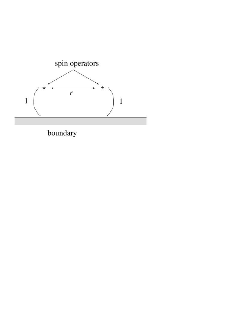
Figure 3: The location of spin operators used in the graph of correlation functions (Fig. 4). We fix the distance of spin operators from the boundary to $1$, and leave the horizontal distance $r$ between them as a variable.

Figure 4: The two-spin correlation for various strength of the defect. We show the result on (a) $\langle\sigma_{1}\sigma_{1}\rangle$ and (b) $\langle\sigma_{1}\sigma_{2}\rangle$ for $\varphi_{0}=0$ (strong coupling and anisotropic limit), $0.1\pi,0.2\pi,0.25\pi$ (no defect) , $0.3\pi,0.4\pi$ and $0.5\pi$ (free boundary condition). They are shown as a function of the distance $r$, in a log-log plot.

From the agreement with the known cases, we believe our exact expressions (165) and (166) of the boundary two-spin correlation are correct, though we made some assumptions during the calculation. While the parameter $u$ is implicitly defined by the eq. (153), there is no essential difficulty in solving the equation numerically. We used Mathematica to solve the equation and then draw graphs of our results. We choose the location of the spins as shown in Fig. 3. We show the correlation functions for various strength of the defect in Fig. 4 as a function of the distance. In the short-distance limit, $\langle\sigma_{1}\sigma_{1}\rangle$ converges to a single power-law which is independent of the defect strength. This is the expected bulk limit. In the large-distance limit, the correlation function is governed by another exponent, which depends on the defect strength. This is the boundary limit. In the next subsection, we will find the boundary exponent actually agrees with the boundary operator with the smallest dimension found in eq. (149). Our result interpolates between these two limits.

In the “short-distance” limit, $\langle\sigma_{1}\sigma_{2}\rangle$ converges to a constant which depends on the defect strength. This actually corresponds to two spins located symmetrically about the defect line, and is related to the one-point function of the bosonic operator $\cos{\varphi}$. In general, $\langle\sigma_{1}\sigma_{2}\rangle$ is smaller than $\langle\sigma_{1}\sigma_{1}\rangle$ for the same defect strength and the same (horizontal) distance, as expected. Nevertheless, they asymptotically converges to the same power-law function in the large-distance limit for $b\neq 0$. Not only the exponent but also the constant prefactor is the same. This somewhat unexpected phenomenon will be further discussed in the next subsection using the boundary OPE.

5.3 Boundary OPE of spin operators

As discussed in Ref. [19], once we obtain the boundary correlation function from the bulk OPE, we can calculate the boundary OPE from the boundary correlation function.

The boundary OPE is the expansion about the boundary limit, where two operators are close to the boundary (real axis). Then the cross-ratio $x$, defined in (152), approaches $1$. Thus we should expand the correlation function in $\tilde{x}=1-x$. If we define $\tilde{u}=e^{2\pi i\tilde{\tau}}$ by

$$\tilde{x}=\left(\frac{\vartheta_{2}(\tilde{u})}{\vartheta_{3}(\tilde{u})}\right)^{4},$$ (173)

$\tilde{u}$ is related to $u=e^{2\pi i\tau}$ by the modular transformation

$$\tilde{\tau}=-\frac{1}{\tau}.$$ (174)

The correlation functions (165) and (166) can be expressed in terms of $\tilde{u}$ by the modular transformation of the elliptic theta function as

$$\langle\sigma_{1}(z_{1},\bar{z}_{1})\sigma_{1}(z_{2},\bar{z}_{2})\rangle = \left(\frac{1}{4y_{1}y_{2}x}\right)^{1/8}\frac{\sqrt{2}\tilde{u}^{(\frac{\varphi_{0}}{\pi})^{2}}}{\vartheta_{3}(\tilde{u})}\vartheta_{3}(\tilde{u}^{-2\varphi_{0}/\pi},\tilde{u}^{2}),$$ (175)

$$\langle\sigma_{1}(z_{1},\bar{z}_{1})\sigma_{2}(z_{2},\bar{z}_{2})\rangle = \left(\frac{1}{4y_{1}y_{2}x}\right)^{1/8}\frac{\sqrt{2}\tilde{u}^{(\frac{\varphi_{0}}{\pi})^{2}}}{\vartheta_{3}(\tilde{u})}\vartheta_{4}(\tilde{u}^{-2\varphi_{0}/\pi},\tilde{u}^{2}).$$ (176)

From these expressions, we can read off the boundary OPE of $\sigma_{1}$ and $\sigma_{2}$. In particular, for both $\langle\sigma_{1}\sigma_{1}\rangle$ and $\langle\sigma_{1}\sigma_{2}\rangle$, the dimension of the intermediate boundary primary operators are given by

$$\Delta_{b}=2n^{2}+\frac{4n\varphi_{0}}{\pi}+2\frac{{\varphi_{0}}^{2}}{\pi^{2}}$$ (177)

where $n$ is an arbitrary integer. They are exactly the boundary scaling dimensions of the primaries in the “moving sector” (148). Thus the “moving sector” is identified as the set of boundary operators generated by the boundary OPE of the spin operators.

We note that, while the intermediate states in the bulk OPE are different for $\sigma_{1}\sigma_{1}$ and $\sigma_{1}\sigma_{2}$, the intermediate states in the boundary OPE are common between them. Only the OPE coefficients are different. Moreover, the OPE coefficient for the boundary operator with the smallest dimension is exactly the same between $\langle\sigma_{1}\sigma_{1}\rangle$ and $\langle\sigma_{1}\sigma_{2}\rangle$. This means that the asymptotic behavior of these two correlation functions at large distance is exactly the same. (For negative $b$, they differ only by their sign.) The only exception is the free boundary case ($b=0$). In this case, there are two boundary operators for each boundary dimension and the two coefficients cancel exactly to make $\langle\sigma_{1}\sigma_{2}\rangle$ identically zero.

The boundary OPE coefficients for $\sigma_{1}\pm\sigma_{2}$ are given by the sum of (or the difference between) those for $\sigma_{1}$ and $\sigma_{2}$. The smallest boundary dimension is given by $2(\frac{\varphi_{0}}{\pi})^{2}$ and $2(1-\frac{\varphi_{0}}{\pi})^{2}$ respectively for $\sigma_{1}+\sigma_{2}$ and $\sigma_{1}-\sigma_{2}$. As discussed in Section 5.1, they are the only relevant boundary operators for this boundary condition.

5.4 Correlation functions of the bosonic operators

Here we consider correlation functions of the bosonic operators $\cos{k\varphi}$. For $k=1$, $\sqrt{2}\cos{\varphi}$ is identified with the composite spin operator $\sigma_{1}\sigma_{2}$ (at the same point). Thus the boundary two-point function of $\cos{\varphi}$ corresponds to a special case of the four-spin correlation function in the presence of the defect line: correlation function of two pairs, each of which consists of two spins located symmetrically about the defect line.

The boundary one-point function can be determined by the method of Ref. [19] as

$$\langle\cos{k\varphi}\rangle=\frac{\cos{k\varphi_{0}}}{(2y)^{1/4}}.$$ (178)

In order to calculate the boundary two-point function $\langle\cos{k\varphi}\cos{k\varphi}\rangle$, we use a kind of mirror image method. Since it is symmetric under $\varphi\rightarrow-\varphi$, it is sufficient to consider only the fixed boundary condition $\varphi=\varphi_{0}$ at the boundary, apart from an ambiguity in the overall constant. The overall constant can not be determined by the mirror image method and will be fixed later by requiring the correct bulk limit.

Given the boundary condition $\varphi=\varphi_{0}$ at the boundary (real axis), the non-chiral boson field $\varphi(z,\bar{z})$ can be represented by a single chiral boson $\phi(z)$ as

$$\varphi(z,\bar{z})=\varphi_{0}+\phi(z)-\phi(z^{\prime}),$$ (179)

where $z^{\prime}$ is the complex conjugate of $z$. Thus the boundary two-point function is mapped to the chiral four-point function as

$$\langle\cos{k\varphi(z_{1},\bar{z}_{1})}\cos{k\varphi(z_{2},\bar{z}_{2})}\rangle=$$ (180)

$$\frac{1}{4}\sum_{\pm\pm}\langle e^{\pm ik[\varphi_{0}+\phi(z_{1})-\phi(z^{\prime}_{1})]}e^{\pm ik[\varphi_{0}+\phi(z_{2})-\phi(z^{\prime}_{2})]}\rangle,$$

where $\pm$’s are summed independently.

Using the standard result on the correlation functions of the vertex operators

$$\langle\prod_{j}e^{i\alpha_{j}\phi(z_{j})}\rangle=\prod_{j<k}(z_{j}-z_{k})^{\alpha_{j}\alpha_{k}/4}\;\;\;\;\;\;(\sum_{j}\alpha_{j}=0),$$ (181)

this reduces to

$$\langle\cos{k\varphi(z_{1},\bar{z}_{1})}\cos{k\varphi(z_{2},\bar{z}_{2})}\rangle=\frac{C}{(4y_{1}y_{2})^{k^{2}/4}}[x^{-k^{2}/4}+x^{k^{2}/4}\cos{2k\varphi_{0}}]$$ (182)

where $C$ is a constant and $y_{1}$, $y_{2}$ and $x$ are defined similarly with eq. (165). Requiring the correct bulk limit

$$\langle\cos{k\varphi(z_{1},\bar{z}_{1})}\cos{k\varphi(z_{2},\bar{z}_{2})}\rangle\rightarrow\frac{1}{2|z_{1}-z_{2}|^{k^{2}/4}},$$ (183)

$C$ is fixed to be $1/2$.

Let us compare our result (182) for $k=1$, which is the special case of four-spin correlation function, with known results. For periodic ($\varphi_{0}=\pi/4$) and antiperiodic ($\varphi_{0}=3\pi/4$) boundary conditions, our result agrees with the bulk four-point spin correlation of the Ising model for the special location of the spins. For the free ($\varphi_{0}=\pi/2$) boundary condition, our result agrees with the square of the boundary two-spin correlation [2] for the free boundary condition. Again we found consistency of our approach with the known results.

5.5 Two-spin correlation near the end of the defect line

Figure 5: The correlation function of two spins located symmetrically about the defect line. It is characterized by the distance from the line $y$ and the angle $\theta$.

So far we have discussed only the defect line without ends (infinitely long or periodic). Let us consider the neighborhood of the end of the defect line. We discuss only the correlation function of two spins located symmetrically about the defect line, as shown in Fig. 5. This can be reduced to the one-point function $\langle\sqrt{2}\cos{\varphi}\rangle=\langle\sigma_{1}\sigma_{2}\rangle$ after the folding, with a changing boundary condition.

We regard the end point as the origin, and make the conformal mapping $z=e^{w}$ to the strip with different boundary conditions at two sides. Then the one-point function is given by the vacuum expectation value with two specified boundary conditions. The Hilbert space of the strip is classified into several sectors by the zero-mode. We only need to consider the lowest energy zero mode to calculate the vacuum expectation value. Thus we fix $\varphi=\varphi_{0}$ at the boundary corresponding to the defect and $\varphi=\pi/4$ at the other boundary.

We employ the mirror image method used in the last subsection. In order to ensure the boundary conditions on the two boundaries, we first need two mirror images as

$$\varphi(w,\bar{w})\sim\frac{\pi}{4}+(\varphi_{0}-\frac{\pi}{4})\frac{v}{\pi}+\phi(w)-\phi(w^{\prime})-\phi(w^{\prime}+2\pi i),$$ (184)

where $\phi$ is a chiral boson, $w^{\prime}$ is the complex conjugate of $w$ and $v={\rm Im}w$. However, the mirror image about one boundary conflicts with the boundary condition on the other boundary. Thus we need the mirror image of the images. In this way, we need infinitely many mirror images as

$$\varphi(w,\bar{w})=\frac{\pi}{4}+(\varphi_{0}-\frac{\pi}{4})\frac{v}{\pi}-\sum_{n}\phi(w^{\prime}+2\pi ni)+\sum_{n}\phi(w+2\pi ni).$$ (185)

Using eq. (181), the one-point function is given by

$$\langle\cos{\varphi}\rangle = \mbox{const.}\cos{[\frac{\pi}{4}+(\varphi_{0}-\frac{\pi}{4})\frac{v}{\pi}]}\left(\prod_{n=-\infty}^{\infty}\frac{2\pi n}{2v+2\pi n}\right)^{1/4}$$ (186)

$$= \mbox{const.}\frac{\cos{[\frac{\pi}{4}+(\varphi_{0}-\frac{\pi}{4})\frac{v}{\pi}]}}{(\sin{v})^{1/4}}.$$

Going back to the half plane, we obtain the one-point function, or the special two-spin correlation before folding as in Fig. 5, near the end of the defect line. It is given by

$$\langle\sigma_{1}(z,\bar{z})\sigma_{2}(z,\bar{z})\rangle=\sqrt{2}\frac{\cos{[\frac{\pi}{4}+(\varphi_{0}-\frac{\pi}{4})\frac{\theta}{\pi}]}}{(2y)^{1/4}},$$ (187)

where $z=0$ is the end of the defect line, $y={\rm Im}z$, $\theta=\arg{z}$, and the overall normalization is determined from the $\theta\rightarrow 0,\pi$ limit. In the $\theta\rightarrow 0$ limit, the spins are located far apart from the defect line and the correlation function should approach the bulk value $(2y)^{-1/4}$. In the $\theta\rightarrow\pi$ limit, the spins are located symmetrically about the defect line and are far apart from the end of the defect. Thus the correlation function should converge to that for the infinitely long defect (178).

5.6 Free energy of the finite length defect line

Here we discuss the free energy due to the presence of the defect line of the continuous Dirichlet universality class (69). A defect line with a finite length corresponds to a finite interval with a different boundary condition, after the folding. The partition function in the presence of the defect line is expressed by the two-point function of a boundary condition changing operator [28]. (For further discussion, see Appendix.)

The dimension of the boundary condition changing operator is determined by the ground-state energy of a strip with boundary conditions corresponding to the defect line and no defect ($b=1$) on the two sides. From the partition function (33), the dimension is found as

$$\Delta_{b}=\frac{1}{2}\left[\frac{1}{\pi}(\varphi_{0}-\frac{\pi}{4})\right]^{2}.$$ (188)

The universal term in the free energy of a defect of length $l$ on an infinite plane is thus given by

$$F_{\rm univ}(l)=-kT\log{Z}=kT\Delta_{b}\log{l}.$$ (189)

The universal free energy of the defect line along the circumference $L$ of a cylinder can be obtained by a conformal mapping $z=\tan{\pi w/L}$ as

$$F_{\rm univ}(l,L)=kT\Delta_{b}\log{\left[\frac{L}{\pi}\sin{\frac{\pi l}{L}}\right]}.$$ (190)

However, the above is not the only term in the free energy. There are also non-universal terms. Firstly, there is a non-universal shift of the ground state energy depending on the boundary condition, as seen in the second term in eqs. (20) and (21). This is due to the phase shift of the fermion momenta (8), which depends on the fermion energy. This effect, which is known as Fumi’s theorem [38] in the general case, depends on the dispersion relation and the phase shift in the entire Brillouin zone, and thus is non-universal. In general, we expect a shift of the ground-state energy of order $1/a$ and the free energy proportional to the defect length as $Al$, where $A$ is a constant of order $1/a$. An exception is the antiferromagnetic defect ($b=-1$). In this case, the quantization of the wavevectors is exactly the same as in the no defect case and only the parity assignment is reversed. Therefore the non-universal term proportional to the length is absent ($A=0$). This is also required from the fact that the antiferromagnetic defect is exactly the two-point correlation of disorder operators [39], which decays purely algebraically.

Secondly, the free energy of the defect line should vanish when there is no defect ($l=0$). Hence a constant term of order $\log{a}$, where $a$ is the cutoff length (lattice constant) is required. The combined result would be approximately $kT\Delta_{b}\log{\frac{l}{a}}$, which is only valid for $l>>a$. The constant term of order $\log{a}$ is non-universal and can be regarded as an effect of the ends of the defect line (or, of the insertion of the boundary condition changing operator.) Moreover, the dependence of the free energy on $l$ when $l\sim a$ should be non-universal. If the defect length approaches to the circumference of the cylinder ($l\sim L$), the dependence on $l$ becomes again non-universal for $(L-l)\sim a$. When $l=L$, however, the defect line completely wraps around the cylinder; there is no longer a non-universal constant due to the ends of the defect line. Nevertheless, a universal constant of order $1$ still remains in general. After the folding, we have a new single boundary condition. The universal remaining constant is nothing but the contribution from the “ground-state degeneracy” [37]: $-kT\log{g}$. In the present problem, $g=1$ for any continuous Dirichlet boundary state, as will be discussed in Section 7. Thus the universal constant for $l=L$ is zero.

As discussed above, the non-universal part in the free energy of the defect line is rather large except for $b=-1$; it may be difficult to measure the universal part in (numerical) experiments. (The dimensions of boundary condition changing operators are measurable in quantum impurity problems [40].)

5.7 Duality and disorder correlation

Our model (1) has a defect line where the strength of vertical (i.e. orthogonal to the defect line) links are altered. Under the duality transformation [41, 22], our model (1) transforms to the Ising model with the defect line where the strength of the horizontal coupling is altered. This “horizontal” model was studied by several authors [6, 7, 8, 9]. The duality transformation exchanges the order and disorder operator. It is illuminating to discuss the duality transformation in the quantum model under the $\tau$-continuum limit. Our “vertical” model corresponds to the quantum Hamiltonian (16). The duality transformation [22] is introduced by defining the new operators $\hat{\mu}$ as in

$$\begin{array}[]{rcl}\hat{\mu}^{z}(n)&\equiv&\prod_{m\leq n}\hat{\sigma}^{x}(m),\\ \hat{\mu}^{x}(n)&\equiv&\hat{\sigma}^{z}(n)\hat{\sigma}^{z}(n+1),\end{array}$$ (191)

where $\hat{\sigma}$’s are defined as in (16). $\hat{\mu}^{z}$ is the disorder operator.

We apply this dual transformation for $-\infty<n<\infty$. Using the new operators $\hat{\mu}$, the Hamiltonian (16) is expressed as

$$H=-\sum_{n\neq 0}\hat{\mu}^{x}(n)-\sum_{n=-\infty}^{\infty}\hat{\mu}^{z}(n-1)\hat{\mu}^{z}(n)-b\hat{\mu}^{x}(0).$$ (192)

Now the Hamiltonian is again the transverse Ising model, but the only the strength of the transverse field is altered at $n=0$. This corresponds to the variation of the horizontal link strength.

Let us consider the model by a perturbation from the model without the defect ($b=1$) as in Ref. [9]. In the continuum limit, the variation of either vertical or horizontal coupling correspond to the perturbation by the same energy density operator. Thus, if the continuum perturbation theory is valid in principle, the “horizontal” model is equivalent to the “vertical” model (1) under some change of the parameter $\varphi_{0}$. Assuming this, the Dirichlet boundary state is transformed to the Dirichlet boundary state with a different parameter $\varphi_{0}$ under the duality transformation. The transformation rule for the parameter $\varphi_{0}$ can be determined from Brown’s relation [9] between the surface exponents of the order/disorder fields:

$$\sqrt{2\Delta_{b}(\sigma)}+\sqrt{2\Delta_{b}(\mu)}=1.$$ (193)

This relation together with our result (149) gives the transformation of $\varphi_{0}$ under the duality transformation:

$$\varphi_{0}\rightarrow\varphi_{0}^{d}=\left\{\begin{array}[]{lr}\frac{\pi}{2}-\varphi_{0}&(0<\varphi_{0}<\frac{\pi}{2})\\ \varphi_{0}-\frac{\pi}{2}&(\frac{\pi}{2}<\varphi_{0}<\pi)\end{array}\right..$$ (194)

Thus the correlation functions of two disorder operators in the Dirichlet boundary state are given by

$$\langle\mu_{j}\mu_{k}\rangle_{D(\varphi_{0})}=\langle\sigma_{j}\sigma_{k}\rangle_{D(\varphi_{0}^{d})}$$ (195)

6 Properties of the continuous von Neumann universality class

Here we discuss the correlation functions near the defect line that is identified with the continuous von Neumann boundary state (113). We also identify the corresponding defect line in the one-dimensional quantum model.

6.1 Two-spin correlation functions

We can calculate the two-spin correlation functions $\langle\sigma_{i}\sigma_{j}\rangle$ in a similar manner to what we did in Section 5.2. The only difference is the boundary state, and consequently the coefficients $A^{\Delta}_{B}$ defined in (155). The boundary state (113) determines the coefficients as

$$A^{(n^{2}/2,A)}_{B}=\left\{\begin{array}[]{ll}1&(n=0)\\ \sqrt{2}\cos{(2n\tilde{\varphi}_{0})}&(n\geq 1)\end{array}\right.$$ (196)

Firstly, it is easy to see that $\langle\sigma_{1}\sigma_{2}\rangle$ vanishes for any value of $\tilde{\varphi}_{0}$, since the bulk OPE $\sigma_{1}$ and $\sigma_{2}$ only generates the operators as in (160).

The bulk OPE coefficients of $\sigma_{j}\sigma_{j}$ ($j=1,2$) are given by

$$C_{\sigma_{1}\sigma_{1}(n^{2}/2,A)} = \sqrt{2}\left(\frac{1}{16}\right)^{n^{2}/2},$$ (197)

$$C_{\sigma_{2}\sigma_{2}(n^{2}/2,A)} = (-1)^{n}\sqrt{2}\left(\frac{1}{16}\right)^{n^{2}/2}.$$ (198)

Thus the correlation functions are given by

$$\langle\sigma_{1}(z_{1},\bar{z}_{1})\sigma_{1}(z_{2},\bar{z}_{2})\rangle$$ (199)

$$= \left(\frac{1}{4y_{1}y_{2}x}\right)^{1/8}\frac{1}{\vartheta_{3}(u)}\sum_{n=0}^{\infty}A^{(n^{2}/2,A)}_{B}C_{\sigma_{1}\sigma_{1}(n^{2}/2,A)}f(\frac{n^{2}}{2},\frac{1}{16},1,x)$$

$$= \left(\frac{1}{4y_{1}y_{2}x}\right)^{1/8}\frac{1}{\vartheta_{3}(u)}(1+\sum_{n=1}^{\infty}2\cos{(2n\tilde{\varphi}_{0})}u^{\frac{n^{2}}{4}})$$

$$= \left(\frac{1}{4y_{1}y_{2}x}\right)^{1/8}\frac{1}{\vartheta_{3}(u)}\vartheta_{3}(e^{2i\tilde{\varphi}_{0}},\sqrt{u}),$$

$$\langle\sigma_{2}(z_{1},\bar{z}_{1})\sigma_{2}(z_{2},\bar{z}_{2})\rangle$$ (200)

$$= \left(\frac{1}{4y_{1}y_{2}x}\right)^{1/8}\frac{1}{\vartheta_{3}(u)}\sum_{n=0}^{\infty}A^{(n^{2}/2,A)}_{B}C_{\sigma_{2}\sigma_{2}(n^{2}/2,A)}f(\frac{n^{2}}{2},\frac{1}{16},1,x)$$

$$= \left(\frac{1}{4y_{1}y_{2}x}\right)^{1/8}\frac{1}{\vartheta_{3}(u)}(1+\sum_{n=1}^{\infty}2(-1)^{n}\cos{(2n\tilde{\varphi}_{0})}u^{\frac{n^{2}}{4}})$$

$$= \left(\frac{1}{4y_{1}y_{2}x}\right)^{1/8}\frac{1}{\vartheta_{3}(u)}\vartheta_{4}(e^{2i\tilde{\varphi}_{0}},\sqrt{u}).$$

They are no longer symmetric under the exchange of $\sigma_{1}$ and $\sigma_{2}$, or equivalently the reflection about the defect line before the folding. We notice that these correlation functions are actually identical to those for the continuous Dirichlet universality class (165,166) for an appropriate value of the parameter. We summarize this observation below

$$\begin{array}[]{rcl}\langle\sigma_{1}\sigma_{1}\rangle_{N(\tilde{\varphi}_{0})}&=&\langle\sigma_{1}\sigma_{1}\rangle_{D(\varphi_{0}=\tilde{\varphi}_{0})}\\ \langle\sigma_{2}\sigma_{2}\rangle_{N(\tilde{\varphi}_{0})}&=&\langle\sigma_{1}\sigma_{1}\rangle_{D(\varphi_{0}=\pi/2-\tilde{\varphi}_{0})}\\ \langle\sigma_{1}\sigma_{2}\rangle_{N(\tilde{\varphi}_{0})}&=&0,\end{array}$$ (201)

where $\langle\rangle_{N(\tilde{\varphi}_{0})}$ and $\langle\rangle_{D(\varphi_{0})}$ are the correlation function in the von Neumann and Dirichlet boundary states, respectively. It is also possible to calculate other quantities discussed in Section 5 for the continuous von Neumann universality class.

6.2 Identification of the defect line

Naively the result $\langle\sigma_{1}\sigma_{2}\rangle=0$ implies that the two layers are completely decoupled. If they are completely decoupled, the boundary state must be $|ff\rangle$ or equivalently the Dirichlet one with $\varphi_{0}=\pi/2$. However, for example, at $\tilde{\varphi}_{0}=\pi/4$ the correlation functions $\langle\sigma_{1}\sigma_{1}\rangle$ and $\langle\sigma_{2}\sigma_{2}\rangle$ behaves exactly as if there is no defect, while $\langle\sigma_{1}\sigma_{2}\rangle$ still vanishes. These behaviours are definitely different from those in $|ff\rangle$ boundary states. Hence there should be some sort of coupling between two layers.

We have not yet found an appropriate defect line in the classical model which corresponds to the continuous von Neumann boundary state. However, we have succeeded in finding an appropriate point defect in the corresponding one-dimensional quantum model. It is given by the Hamiltonian:

$$H=-\sum_{n\neq 0}\hat{\sigma}^{x}(n)-\sum_{n\neq 0}\hat{\sigma}^{z}(n-1)\hat{\sigma}^{z}(n)-b\hat{\sigma}^{z}(-1)\hat{\sigma}^{x}(0),$$ (202)

where the operators are defined similarly as in eq. (16).

We show that this model is related to the previous model (16) by a duality transformation (191) on one side of the defect only. The duality transformation on the half-line $n\geq 0$ is defined by

$$\hat{\mu}^{z}(n) \equiv \prod_{0\leq m\leq n}\hat{\sigma}^{x}(m),$$ (203)

$$\hat{\mu}^{x}(n) \equiv \hat{\sigma}^{z}(n)\hat{\sigma}^{z}(n+1).$$ (204)

The new operators $\hat{\mu}$’s are defined only for $n\leq 0$ and commute with $\hat{\sigma}$’s at $n<0$. They obey the same commutation relation as the original $\hat{\sigma}$’s do. The Hamiltonian (202) is rewritten as

$$H = -\sum_{n<0}\hat{\sigma}^{x}(n)-\sum_{n\geq 0}\hat{\mu}^{x}(n)$$ (205)

$$-\sum_{n<0}\hat{\sigma}^{z}(n-1)\hat{\sigma}^{z}(n)-\sum_{n>0}\hat{\mu}^{z}(n-1)\hat{\mu}^{z}(n)$$

$$-b\hat{\sigma}^{z}(-1)\hat{\mu}^{z}(0).$$

This is exactly the Hamiltonian (16), under the redefinition $\hat{\mu}\rightarrow\hat{\sigma}$.

In this way, the correlation functions in our model $\langle\rangle_{M}$ are identified with the correlation functions in the Dirichlet boundary condition as follows:

$$\langle\sigma_{1}\sigma_{1}\rangle_{M} = \langle\sigma_{1}\sigma_{1}\rangle_{D(\varphi_{0})},$$ (206)

$$\langle\sigma_{2}\sigma_{2}\rangle_{M} = \langle\mu_{2}\mu_{2}\rangle_{D(\varphi_{0})}$$ (207)

$$= \langle\sigma_{1}\sigma_{1}\rangle_{D(\varphi_{0}^{d})},$$

$$\langle\sigma_{1}\sigma_{2}\rangle_{M} = \langle\sigma_{1}\mu_{2}\rangle_{D(\varphi_{0})}=0,$$ (208)

where $\mu$ is the disorder operator [39], $\varphi_{0}^{d}$ is defined in (194) and $\varphi_{0}$ is determined by the parameter $b$ as in (70).

These results exactly agree with the correlation functions (201) in the von Neumann boundary condition if $\varphi_{0}=\tilde{\varphi}_{0}$. Therefore our model (202) presumably corresponds to the continuous von Neumann boundary state (113) in the continuum limit.

7 Renormalization group flow among the boundary states

7.1 The relative stability of the boundary states

Now we discuss the relative stability and the renormalization group flow among the boundary states. In this section, the orbifold radius $r$ is again fixed to $1$ as we discuss the Ising defect problem. The universal “ground-state degeneracy” $g$ [37], which is given by the inner product of the boundary state and the ground state, turns out to be $1$ in the continuous Dirichlet boundary state (111) for any value of $\varphi_{0}$. Similarly, $g=\sqrt{2}$ in the continuous von Neumann boundary state (113) independent of $\tilde{\varphi}_{0}$. The number $g$ plays the role similar to the central charge $c$ in the bulk conformal field theory. According to the “$g$-theorem” [37], $g$ decreases along a renormalization group trajectory connecting two conformally invariant boundary conditions.

In (111) and (113), the boundary state depends continuously on the defect strength $b$, namely there is a fixed line of conformally invariant boundary conditions. Thus it is natural that $g$ is constant along two continuous line of boundary universality class, as central charge $c$ is constant along a fixed line of conformally invariant bulk theories. Namely, no renormalization group flow can occur along these lines. The values of $g$ in the 8 discrete boundary states are simply the product of $g$ for the two Ising layers. It is known [28] that $g=1$ for the free Ising boundary condition and $g=1/\sqrt{2}$ for the fixed Ising boundary condition. Thus $g$ is $1/\sqrt{2}$ for the endpoint Neumann boundary states ($|\uparrow f\rangle$ etc.) and $1/2$ for the endpoint Dirichlet boundary states ($|\uparrow\uparrow\rangle$).

By the “$g$-theorem”, the continuous Neumann boundary state is the most unstable among these boundary states. The next most unstable one is the continous Dirichlet, then the endpoint Neumann, and the most stable ones are the endpoint Dirichlet. If there is no restriction on the defect line, it is thus generically attracted to one of the endpoint Dirichlet boundary states. In order to realize the other universality classes, we must protect the defect line from the relevant operators, for example by an appropriate symmetry. From the expression of the boundary states as the tensor products of the Ising boundary states, it is clear that the discrete endpoint boundary states break the global $Z_{2}$ symmetry: $\sigma\rightarrow-\sigma$. Thus if we do not break the global $Z_{2}$ symmetry, the defect line is renormalized to one of the continuous states. On the other hand, the endpoint Neumann boundary states are expected to have a different $Z_{2}$ symmetry: Ising spin flip only on the one side of the defect line. For example, $|\uparrow f\rangle$ is invariant under the Ising spin flip in the second layer. Therefore the defect line will be renormalized into one of the endpoint Neumann ones if we break the global $Z_{2}$ symmetry but preserve the other $Z_{2}$ symmetry.

Analysis of the operator contents is useful to further investigation of this problem. We can obtain the spectrum of the boundary operators in the continuous Neumann boundary states in a similar manner as in Section 5.1. The partition function on the strip with the same Neumann boundary on both sides is given by

$$Z=\frac{1}{\eta(q)}\sum_{n=-\infty}^{\infty}q^{n^{2}/2}+\frac{1}{\eta(q)}\sum_{n=-\infty}^{\infty}q^{(n+2\tilde{\varphi}_{0}/\pi)^{2}/2},$$ (210)

where $q$ is defined as in (26).

From this expression, we can read off the whole spectrum of boundary operators. In particular, the dimensions of the relevant operators (other than the identity) are given by $1/2$ (twice), $2(\frac{\tilde{\varphi}_{0}}{\pi})^{2}$, $\frac{1}{2}(1-\frac{2\tilde{\varphi}_{0}}{\pi})^{2}$. From the two-spin correlation functions (201), the latter two are identified with the spin operators $\sigma_{1}$ and $\sigma_{2}$. The remaining two with dimension $1/2$ are identified with $\sigma_{1}\sigma_{2}$. The multiplicity $2$ is understood as follows. Since the dimension $1/2$ is independent of the parameter $\tilde{\varphi}_{0}$, we may consider the simplest case $b=1$ ($\tilde{\varphi}_{0}=\pi/4$). At this point, the problem is reduced to the Ising model without any defect after the duality transformation. Now we can unfold the system and reduce the boundary OPE between $\sigma_{1}$ and $\sigma_{2}$ to the bulk OPE between $\sigma$ and $\mu$, which is given [39, 42] as

$$\sigma(w,\bar{w})\mu(0,0)\sim w^{3/8}\bar{w}^{-1/8}\psi+w^{-1/8}\bar{w}^{3/8}\bar{\psi}.$$ (211)

Thus there are actually two operators $\psi$ and $\bar{\psi}$ generated by the OPE of $\sigma$ and $\mu$. The coefficients depend on the relative location of $\sigma$ and $\mu$. Translating to the folded picture, two boundary operators are generated by the OPE of $\sigma_{1}$ and $\sigma_{2}$ and the relative coefficients depend on the location of $\sigma_{1}$ and $\sigma_{2}$. While the above argument is only valid for the special point $b=1$, it is natural to expect that two boundary operators are generated by the OPE for any value of $b$ (or $\tilde{\varphi}_{0}$).

Now let us turn to the stability of the Neumann boundary state. Since the spin operators $\sigma_{1}$ and $\sigma_{2}$ are relevant, the perturbation by these operators will drive the system away from the von Neumann boundary state. The resulting state will be one of the discrete boundary states. For example, if we perturb by $\sigma_{1}$, the boundary will be presumably renormalized to $|\uparrow f\rangle$ (or $|\downarrow f\rangle$) boundary state. The remaining relevant operators are generated by $\sigma_{1}\sigma_{2}$. Under this perturbation, the boundary will be presumably renormalized to the Dirichlet boundary state with some value of $\tilde{\varphi}_{0}$. These conclusions are consistent with our discussion based on the “$g$-theorem”.

To achieve the continuous Neuman boundary state in the infrared limit, we must protect the boundary from these relevant operators. The model (202) has the following $Z_{2}\times Z_{2}$ symmetry:

$$\begin{array}[]{ccc}\hat{\sigma}^{z}(n)\rightarrow-\hat{\sigma}^{z}(n)&(n<0)&\;\;\;\mbox{with}\;\;\hat{\sigma}^{x}(0)\rightarrow-\hat{\sigma}^{x}(0)\\ \hat{\sigma}^{z}(n)\rightarrow-\hat{\sigma}^{z}(n)&(n\geq 0)\end{array}$$ (212)

In the continuum limit, it may be simply interpreted as

$$\sigma_{1}\rightarrow-\sigma_{1}\;\;\mbox{and}\;\;\sigma_{2}\rightarrow-\sigma_{2}.$$ (213)

Any of the relevant operators $\sigma_{1}$, $\sigma_{2}$ and $\sigma_{1}\sigma_{2}$ breaks this $Z_{2}\times Z_{2}$ symmetry. This means that the $Z_{2}\times Z_{2}$ symmetry protects the von Neumann boundary state. However, the Dirichlet boundary state with $\varphi_{0}=\pi/2$ (i.e. $|ff\rangle$) also has the $Z_{2}\times Z_{2}$ symmetry. Hence a defect line with the $Z_{2}\times Z_{2}$ symmetry may not renormalize into the von Neumann boundary state; an obvious example is our original model (1) with $b=0$.

As we have discussed, the $\sigma_{1}\sigma_{2}$ perturbation will presumably drive the defect line to the Dirichlet boundary state, where only the single global $Z_{2}$ symmetry $\sigma_{1,2}\rightarrow-\sigma_{1,2}$ exists. This is natural since $\sigma_{1}\sigma_{2}$ breaks the $Z_{2}\times Z_{2}$ symmetry to $Z_{2}$. On the other hand, the reflection symmetry $\sigma_{1}\leftrightarrow\sigma_{2}$, which was absent in the continuous Neumann boundary state, is recovered in the continuous Dirichlet boundary state.

The boundary operator content in the continuous Dirichlet boundary state is given in Section 5.1. The two boundary operators with the dimensions $2(\varphi_{0}/\pi)^{2}$ and $2[(\pi-\varphi_{0})/\pi]^{2}$ are only the relevant boundary operators. As we have shown in Section 5.3, they correspond to $\sigma_{1}\pm\sigma_{2}$. At the “periodic” point $\varphi_{0}=\pi/4$, $\Delta_{b}=1/8,9/8$ which correspond to $\sigma$ and $d\sigma/dx\sim(\sigma_{1}-\sigma_{2})/a$. At the “free” point $\varphi_{0}=\pi/2$, $\Delta_{b}=1/2,1/2$ since $\sigma_{1}$ and $\sigma_{2}$ are independent.

Thus, if we preserve the global $Z_{2}$ symmetry $\sigma_{1},\sigma_{2}\rightarrow-\sigma_{1},-\sigma_{2}$, the fixed line is stable. If we perturb the defect line by the relevant operator $\sigma_{1}\pm\sigma_{2}$, the boundary state will be presumably renormalized to one of the magnetized boundary states ($|\uparrow\uparrow\rangle$ etc.) Such a flow is established at the “free” point ($\varphi_{0}=\pi/2$), where the boundary condition of the two independent Ising models are renormalized. We expect the renormalization group flow from the entire fixed line to the discrete magnetized boundary states, consistently with our arguments based on “$g$-theorem”.

8 Generalized defects and universality

Grimm [16] considered generalizations of the defect line. Here we discuss his result from our general consideration of defect universality classes.

His first (“integrable”) generalization of the defect line is given by the quantum Hamiltonian

$$H(\alpha,\phi)=-\sum_{j=1}^{N-1}\left[\sigma_{j}^{x}+\sigma_{j}^{z}\sigma_{j+1}^{z}\right]-\left[\sigma_{N}^{x}+\alpha\sigma_{N}^{\phi}\sigma_{1}^{\phi}\right]$$ (214)

where

$$\sigma^{\phi}\equiv\cos{\phi}\sigma^{z}+\sin{\phi}\sigma^{y}.$$ (215)

(Eq. (214) corresponds to eq. (3.1) in Ref. [16] but we have changed the notation.) When $\phi=0$, this reduces to the “ordinary” defect described by eq. (16). Grimm obtained the exact spectrum of this model. Apart from the non-universal shift in the ground-state energy, the result was identical to the “ordinary defect”, i.e. continous Dirichlet boundary state (111) with some value of $\varphi_{0}$. He noticed that the model (214) preserves the global $Z_{2}$ symmetry (simultaneous rotation about $x$-axis by angle $\pi$ at each site) and thus it belongs to the same universality class as the “ordinary” one (16). These are completely consistent with our arguments based on “$g$-theorem” and the boundary operator contents.

He further introduced another generalization given by

$$H(\beta,\psi)=-\sum_{j=1}^{N-1}\left[\sigma_{j}^{x}+\sigma_{j}^{z}\sigma_{j+1}^{z}\right]-\left[\sigma_{N}^{x}+\beta\sigma_{N}^{z}(\cos{\psi}\sigma_{1}^{z}-\sin{\psi}\sigma_{1}^{x})\right],$$ (216)

where $0<\psi<\pi$. (This corresponds to eq. (4.1) in Ref. [16] but again we changed the notation.) This model is not exactly solvable and he obtained the spectra numerically. He calculated the difference of the universal term in the ground-state energy between (216) with $\beta>0$ and eq. (16) with $b=0$. The numerical result was consistent with his conjecture that the difference is given by $0,1/16$ and $1/2$ (in unit of $2\pi v/N$), respectively for $\psi<\pi/2$, $\psi=\pi/2$ and $\psi>\pi/2$ (independent of $\beta$ as long as $\beta>0$.) He argued that this means that there are three universality classes for this model.

Let us reconsider his model (216) from our viewpoint. As he noticed, this model no longer keeps the global $Z_{2}$ symmetry. From our arguments in the previous subsection, we expect that the defect line will generically renormalize into one of the endpoint Dirichlet boundary states. Actually, we can understand as follows. (Here we restrict to the case in which $\beta>0$.) We expect $\langle\sigma_{1}^{x}\rangle>0$ due to the transverse field in the Hamiltonian (216). Thus $\langle\sigma_{N}^{z}\rangle$ is expected to be negative for all $0<\psi<\pi$, due to the effective field generated by $\sigma_{1}^{x}$. Then $\sigma_{1}^{z}$ is affected by the effective field generated by $\sigma_{N}^{z}$. Depending on the sign of the coupling, $\langle\sigma_{1}^{z}\rangle$ should be negative for $0<\psi<\pi/2$ and positive for $\pi/2<\psi<\pi$. At $\psi=\pi/2$, neither direction is favored for $\sigma_{1}^{z}$.

Thus we expect that the corresponding boundary state is $|\downarrow\downarrow\rangle$, $|\downarrow f\rangle$ and $|\downarrow\uparrow\rangle$, respectively for $0<\psi<\pi/2$, $\psi=\pi/2$ and $\pi/2<\psi<\pi$. From the discussion of the previous subsection, the endpoint Neumann boundary state $|\downarrow f\rangle$ is unstable and would be realized only at $\psi=\pi/2$. Actually, at this point we have the extra $Z_{2}$ symmetry: $\sigma^{z}\rightarrow-\sigma^{z}$ only on one side of the defect. This symmetry protects the endpoint Neumann boundary state, as we argued. Changing $\psi$ from $\pi/2$ corresponds to the relevant perturbation and the defect line will renormalize to the endpoint Dirichlet: $|\downarrow\downarrow\rangle$ or $|\downarrow\uparrow\rangle$ depending on the direction of the perturbation. We also note that, although his model (216) at $\psi=\pi/2$ looks similar to our model (202) which corresponds to the continuous von Neumann boundary state, they are actually different. The transverse field at site $n=0$ exists in the former, breaking the $Z_{2}\times Z_{2}$ symmetry (212) to the single $Z_{2}$ symmetry.

Grimm calculated the ground-state energy of the model (216) on a circle. In our formalism, it corresponds to a strip of width $N/2$, with the defect boundary state on one side and the “periodic” (Dirichlet with $\varphi_{0}=\pi/4$) boundary state on the other side. The partition function of the system is readily derived; only the untwisted sector of the defect boundary states contributes to the partition function. From the partition function, the ground-state energy of the strip is given by $1/16,1/8$ and $9/16$ in the unit of $2\pi v/N$, respectively for $|\downarrow\downarrow\rangle$, $|\downarrow f\rangle$ and $|\downarrow\uparrow\rangle$. Following his definition, we subtract the ground-state energy in the case the defect boundary state is $|ff\rangle$, to obtain $0,1/16$ and $1/2$ respectively for those three cases. Thus our analysis is in complete agreement with Grimm’s. Furthermore, his conjecture based on $c=1/2$ character of the Virasoro algebra also agrees with our boundary states which is tensor products of Ising boundary states.

The “new” universality class of the defect lines he obtained was actually equivalent to boundary conditions of two independent Ising models. Nevertheless, his general discussion on the universality of the defect lines seems quite correct.

Recently, Karevski and Henkel [44] discussed another kind of generalization. They studied a junction of $S=1/2$ and $S=1$ quantum Ising chains. In the continuum limit, the bulk universality class of the $S=1$ Ising chain is identical to that of standard $S=1/2$ Ising model [45]. Thus, when both chains are critical, we expect that the universality class of the junction is identical to that of the defect discussed in this paper. Actually, they numerically studied [44] the junction with the Ising $Z_{2}$ symmetry, and found the universal behaviour corresponding to the continuous Dirichlet boundary condition in our terminology. This also confirms that the notion of universality applies to the defect problem.

9 Summary and Discussion

We studied the continuum limit of the two-dimensional critical Ising model with a defect line. Folding the system at the defect line, we map the system to the critical Ashkin-Teller model [25, 30] at the decoupling point with boundaries. Thus we can classify the universality classes of the defect lines by the boundary states of a conformal field theory.

Based on the exact partition function, we identified the boundary state corresponding to arbitrary strength of the defect, in terms of the Ashkin-Teller Ishibashi states. Furthermore, we discussed the possible boundary states in the $Z_{2}$ orbifold of free boson, which is identified with the continuum limit of the critical Ashkin-Teller model. There are two continuous lines of boundary states, and eight discrete ones for general values of the compactification radius $r$. The special case $r=1$ is applied to our problem of the defect lines in the Ising model. It is shown that the obtained orbifold boundary states include all the known defect lines, and one new one-parameter family universality class of defect lines corresponding to the orbifold von Neumann boundary state. We conjectured that the above boundary states exhausts all the possible boundary states on $Z_{2}$ orbifold for generic value of $r$; if this is true, we have identified the complete set of universality classes of defect lines in the Ising model.

From the boundary state, we obtained the complete spectrum of boundary operators. We calculated the exact boundary two-spin correlation functions for arbitrary strength of the defect, employing the method of Cardy and Lewellen [19] and Zamolodchikov’s solution [20] for $c=1$ conformal block of spin operators. We also calculated the boundary two-point functions of bosonic operators, one of which is identified as a special case of the four-spin correlation function. In addition, we obtained a special case of the two-spin correlation function near the end of the defect line, the universal term in the free energy of the defect line and the correlation function of the disorder operators. While we made some assumptions during the calculation, our approach, which satisfies several nontrivial consistency check, appears to be valid.

We also calculated the two-point spin correlation functions in the new one-parameter family of defect lines, and identified the corresponding quantum model using the duality transformation. For the 8 discrete universality classes, calculation of the correlation functions reduces to that in the Ising model with a boundary, which is already solved [19]. Thus we have obtained two-point spin correlation functions for all defect universality classes found so far (i.e. for all the universality classes, if our conjecture is correct.) Finally, we discussed the renormalization-group flow among the defect universality classes based on the “$g$-theorem” and the operator contents. We explained Grimm’s results on the generalized defects, applying our observations.

A possible extention of our present work is the analysis of the boundary states in the general critical Ashkin-Teller model, i.e. for general value of the compactification radius of the orbifold. While two continuous families and eight discrete boundary states exist in general, their relative stability will vary. Moreover, for special values of the radius, additional boundary states may appear, as in the case of the free boson [43].

In Ref. [4], the first attempt was made to apply boundary conformal field theory to the defect problem via folding. However, it was essentially reproduction of the earlier results. On the other hand, our present result provides a more detailed description of defect lines in the Ising model, than that in the earlier literatures. This demonstrates the power of boundary conformal field theory for the application to the defect problems. In particular, the solution indeed posesses $c=1$ structure which is absent in the original $c=1/2$ problem before the folding. Thus the folding seems a really necessary procedure to treat the defect problem in terms of conformal field theory. From the general viewpoint on boundary conformal field theory, the present model seems one of the simplest nontrivial models with an infinite number of boundary conformal towers. Cardy’s original treatment [2, 28] mainly focused on minimal models which have a finite number of conformal towers. Most of the successful applications [3] to $c\geq 1$ have also been to theories with a finite number of primaries with respect to current algebra. When the number of primaries cannot be reduced to a finite one, there are several technical difficulties [4]. In spite of those difficulties, we found that the present problem is tractable, though we have not yet completely understood the structure of the theory as we do in minimal models. We hope that the observations on the present model will be useful in the further development of boundary conformal field theory with infinitely many conformal towers.

Appendix: free energy and the boundary condition changing operator

By folding, a finite length defect line is mapped to a changed boundary condition for a finite interval. Let us discuss the free energy associated to such a finite interval of changed boundary condition. Using the transfer matrix (Hamiltonian) in the direction parallel to the boundary (defect line), the partition function of the system may be written as

$$Z(l)={\rm Tr}e^{-(L-l)H_{0}}e^{-lH_{D}},$$ (217)

where $l$ is the interval of the changed boundary condition (length of the defect), $L$ is the system size in the direction parallel to the boundary and $H_{0}$ and $H_{D}$ are Hamiltonian for the original and changed boundary conditions. The partition function in the absence of the defect line is

$$Z_{0}={\rm Tr}e^{-LH_{0}}.$$ (218)

On the other hand, a change in the boundary condition can be associated with a “boundary condition changing operator” [28]. The boundary condition changing operator acts in an enlarged Hilbert space with all possible boundary conditions, and maps a whole subspace with a particular boundary condition into each other. By the boundary condition changing operator $U$, the Hamiltonian is mapped as

$$U^{\dagger}H_{0}U=H_{D}$$ (219)

In their pioneering work, Schotte and Schotte [47] introduced such an operator for the free boson. (See also [40].) Here we discuss the non-orbifold free boson. The boundary condition changing operator that maps the Dirichlet boundary condition $\varphi=0$ to the Dirichlet boundary condition with a different boundary value $\varphi=\delta$ is given as

$$U=\exp{\left[i\frac{\delta}{\pi}\tilde{\varphi}(0)\right]},$$ (220)

where $\tilde{\varphi}(0)$ is the quantum operator corresponding to the $\tilde{\varphi}$ at the boundary. Here the operators are quantized, regarding the direction parallel to the boundary as a imaginary time. As they claimed, $U$ is apparently a unitary operator. Then it follows

$$U^{\dagger}e^{-lH_{0}}U=e^{-lH_{D}},$$ (221)

and thus

$$Z(l)={\rm Tr}\left[e^{-(L-l)H_{0}}U^{\dagger}e^{-lH_{0}}U\right].$$ (222)

Namely, the ratio of $Z(l)$ and $Z_{0}$ is identified with the two-point correlation function of the boundary condition changing operator:

$$\frac{Z(l)}{Z_{0}}=\langle U^{\dagger}(l)U(0)\rangle,$$ (223)

where the expectation value is defined in the original theory with the Hamiltonian $H_{0}$. In the following, we assume the thermodynamic limit $L\rightarrow\infty$. The asymptotic behavior for large $l$ is governed by the lowest dimension $\Delta_{b}$ of the boundary condition changing operator. This gives

$$\langle U^{\dagger}(l)U(0)\rangle\sim\mbox{const.}l^{-\Delta_{b}}$$ (224)

The free energy of the changed boundary condition (defect line) of a finite length is given by taking the logarithm as

$$F(l)=-kT\log{\frac{Z(l)}{Z_{0}}}=\mbox{const.}+kT\Delta_{b}\log{l}.$$ (225)

The constant term is non-universal. From the dimensional analysis, we expect it to depend on the short-distance cutoff (lattice spacing) $a$ as roughly $-\log{a}$ In general, there can be also a non-universal shift in the energy for a different boundary condition. This contributes extra $Al$, where $A$ is a non-universal constant of order $1/a$, to the free energy.

However, there is a subtlety in the above argument: $U$ cannot be a unitary operator in the standard sense, since $H_{0}$ and $H_{D}$ have different spectrum in general. This peculiarity is presumably related to the presence of infinite degrees of freedom in the field theory. Thus the identity (221) and the above argument may be questionable. We argue that $U$ is still a unitary operator in some weak sense and the above discussion on free energy is valid in general. For the free boson case, we can demonstrate the validity by calculating both sides of the equation (223) independently.

Let us consider the free boson with the Lagrangian (35). We take the boundary as $x$-axis ($y=0$) and assume that the system lies in the upper half plane. We consider the Dirichlet boundary condition $\varphi=\delta$ for the interval $0<x<l$, and $\varphi=0$ elsewhere. The corresponding boundary condition changing operator is given in (220). The asymptotic form of the two-point correlation function of the boundary condition changing operator is given by (224) with $\Delta_{b}=\delta^{2}/\pi^{2}$. On the other hand, the Free energy in the absence of the changed boundary condition is given by

$$Z_{0}=\int{\cal D}\varphi e^{-\frac{1}{2\pi}\int d^{2}x(\partial_{\mu}\varphi)^{2}},$$ (226)

where $\varphi=0$ at the boundary ($y=0$). In the presence of the changed boundary condition, we write

$$\varphi=\varphi_{c}+\varphi_{q},$$ (227)

where $\varphi_{c}$ satisfies

$$\partial^{2}\varphi_{c} = 0$$

$$\varphi_{c}(x,0) = \left\{\begin{array}[]{cl}0&(x<0,l<x)\\ \delta&(0<x<l)\end{array}\right.$$ (230)

$$\varphi_{c}(x,y) \rightarrow 0\;\;\;(y\rightarrow\infty)$$

$\varphi_{q}$ is only required to satisfy $\varphi_{q}=0$ at the boundary, which is exactly the same condition $\varphi$ obeyed in the absence of the changed boundary condition. In other words, the change in the boundary condition is completely absorbed by $\varphi_{c}$. The partition function in the presence of the changed boundary condition is given as

$$Z(l)=\int{\cal D}\varphi_{q}e^{-\frac{1}{2\pi}\int d^{2}x[\partial_{\mu}(\varphi_{q}+\varphi_{c})]^{2}}.$$ (231)

The action can be decoupled as

$$\frac{1}{2\pi}\int d^{2}x(\partial_{\mu}\varphi_{c})^{2}+(\partial_{\mu}\varphi_{q})^{2},$$ (232)

since the cross term is shown to vanish by partial integration. Actually there is an infinite number of solution for $\varphi_{c}$ and we must sum over such allowed $\varphi_{c}$, apart from the integration over $\varphi_{q}$. However, in the large-$l$ limit, only the one with minimum action dominates. For $|\delta|<\pi r$, $\varphi_{c}$ with minimum action is given by

$$\varphi_{c}=\frac{\delta}{\pi}\left(\tan^{-1}{\frac{y}{x-l}}-\tan^{-1}{\frac{y}{x}}\right).$$ (233)

(The ones with larger value of the action is given by replacing $\delta$ by $\delta+2\pi r$, etc.) The leading term in the partition function is given by

$$Z(l) = \int{\cal D}\varphi_{q}\exp{[-\frac{1}{2\pi}\int d^{2}x(\partial_{\mu}\varphi_{c})^{2}+(\partial_{\mu}\varphi_{q})^{2}]}$$ (234)

$$= \exp{[-\frac{1}{2\pi}\int d^{2}x(\partial_{\mu}\varphi_{c})^{2}]}\int{\cal D}\varphi_{q}\exp{[-\frac{1}{2\pi}\int d^{2}x(\partial_{\mu}\varphi_{q})^{2}]}$$

The functional integral over $\varphi_{q}$ is identical to $Z_{0}$ in eq. (226). The action of $\varphi_{c}$ can be calculated using the explicit form (233). Actually it diverges at the singularities $(x,y)=(0,0)$ and $(l,0)$. Introducing the short-distance cutoff $a$, we obtain

$$\frac{1}{2\pi}\int d^{2}x(\partial_{\mu}\varphi_{c})^{2}=\frac{\delta^{2}}{\pi^{2}}\log{\frac{l}{a}}.$$ (235)

Thus we finally get

$$\frac{Z(l)}{Z_{0}}=(\frac{a}{l})^{\delta^{2}/\pi^{2}},$$ (236)

which agrees with the two-point correlation function of the boundary condition changing operator. Thus the validity of the relation (223) is explicitly shown in the free boson case.

This calculation can be generalized to the orbifold boson. On the other hand, in general conformal field theories, it is difficult to calculate directly the partition function in the presence of the changed boundary condition. We expect that the relation (223) also holds in such general cases.

References

• [1] K. Binder, in Critical behavior at surfaces, Phase transitions and critical phenomena vol. 8, edited by C. Domb and J. Lebowitz (Academic Press, London, 1983).
• [2] J. L. Cardy, Nucl. Phys. B 240, 514 (1984).
• [3] I. Affleck, Acta Physica Polonica, 26, 1869 (1995).
• [4] E. Wong and I. Affleck, Nucl. Phys. B 417, 403 (1994).
• [5] L. Onsager, Phys. Rev. 65, 117 (1944).
• [6] R. V. Bariev, Sov. Phys. JETP 50, 613 (1979).
• [7] B. M. McCoy and J. H. H. Perk, Phys. Rev. Lett. 44, 840 (1980).
• [8] L. P. Kadanoff, Phys. Rev. B 24, 5382 (1981).
• [9] A. C. Brown, Phys. Rev. B 25, 331 (1982).
• [10] L. Turban, J. Phys. A 18, L325 (1985).
• [11] L. G. Guimarães and J. R. Drugowich de Felício, J. Phys. A. 19, L341 (1986).
• [12] M. Henkel and A. Patkós, Nucl. Phys. B 285, 29 (1987).
• [13] M. Henkel, A. Patkós and M. Schlottmann, Nucl. Phys. B 314, 609 (1989).
• [14] G. G. Cabrera and R. Julien, Phys. Rev. B 35, 7062 (1987).
• [15] D. B. Abraham, L. F. Ko, and N. M. Svrakic, J. Stat. Phys. 56, 563 (1989).
• [16] U. Grimm, Nucl. Phys. B 340, 633 (1990).
• [17] G. Delfino, G. Mussardo and P. Simonetti, Nucl. Phys. B 432, 518 (1994).
• [18] M. Oshikawa and I. Affleck, Phys. Rev. Lett. 77, 2604 (1996).
• [19] J. L. Cardy and D. C. Lewellen, Phys. Lett. B 259, 274 (1991).
• [20] Al. B. Zamolodchikov, Sov. Phys. JETP 63, 1061 (1986).
• [21] T. D. Schultz, D. C. Mattis, and E. H. Lieb, Rev. Mod. Phys. 36, 856 (1964).
• [22] E. Fradkin and L. Susskind, Phys. Rev. D 17, 2637 (1978).
• [23] A. Luther and I. Peschel, Phys. Rev. B 12, 3908 (1975).
• [24] J. B. Zuber and C. Itzykson, Phys. Rev. D 15, 2775 (1977).
• [25] J. Ashkin and E. Teller, Phys. Rev. 64, 178 (1943).
• [26] P. Ginsparg, in Fields, Strings and Critical Phenomena, Les Houches, Session XLIX, edited by E. Brezin and J. Zinn-Justin (North-Holland, Amsterdam, 1988).
• [27] N. Ishibashi, Mod. Phys. Lett. A 4, 251 (1989).
• [28] J. L. Cardy, Nucl. Phys. B 324, 581 (1989).
• [29] J. L. Cardy, Nucl. Phys. B 275, 200 (1986).
• [30] S. K. Yang, Nucl. Phys. B 285, 183 (1987).
• [31] V. G. Kac, in Lecture Notes in physics Vol. 94 (Springer, New York, 1979)
• [32] J. A. Harvey and J. A. Minahan, Phys. Lett. B 188, 44 (1987).
• [33] N. Ishibashi and T. Onogi, Nucl. Phys. B 318, 239 (1989).
• [34] G. Pradisi and A. Sagnotti, Phys. Lett. B 216, 59 (1989).
• [35] C. G. Callan, C. Lovelace, C. R. Nappi, and S. A. Yost, Nucl. Phys. B 293, 83 (1987).
• [36] D. Friedan, private communications
• [37] I. Affleck and A. W. W. Ludwig, Phys. Rev. Lett. 67, 161 (1991).
• [38] G. D. Mahan, Many-particle physics 2nd ed. (Plenum Press, New York, 1990).
• [39] L. P. Kadanoff and H. Ceva, Phys. Rev. B 3, 3918 (1971).
• [40] I. Affleck and A. W. W. Ludwig, J. Phys. A 27, 5375 (1994).
• [41] H. A. Kramers and G. H. Wannier, Phys. Rev. 60, 252 (1941).
• [42] A. A. Belavin, A. M. Polyakov and A. B. Zamolodchikov, Nucl. Phys. B 241, 333 (1984).
• [43] C. G. Callan, C. Lovelace, C. R. Nappi and J. M. Maldacena, Nucl. Phys. B422, 417 (1994).
• [44] D. Karevski and M. Henkel, preprint cond-mat/9610079.
• [45] W. Hofstetter and M. Henkel, J. Phys. A 29, 1359 (1996).
• [46] A. W. W. Ludwig (unpublished).
• [47] K. D. Schotte and U. Schotte, Phys. Rev. 182, 479 (1969).