How to observe distinct universal conductances in tunneling to quantum Hall states: having the right contacts

Abstract

We show that different universal values can be obtained for the two-terminal conductance of a fractional quantum Hall state. At large voltages, or strong coupling, the conductance of a point-like tunneling junction between an electron gas reservoir and a Laughlin FQH state at filling fraction $\nu$ saturates to a universal value $G={\frac{2\nu}{\nu+1}}{\frac{e^{2}}{h}}$. We use this result to show that devices with different types of contacts between the reservoir and the FQH state lead to distinct universal values of saturation conductance which are rational multiples of $e^{2}/h$. The particular fraction $e^{2}/h$ is obtained for the case of electron tunneling in and out of a FQH liquid through two point contacts. We demonstrate that the problem of tunneling between an electron gas and a fractional quantum Hall state through an impurity is exactly equivalent to the problem of tunneling between a chiral Fermi liquid and a chiral Luttinger liquid. We investigate in detail the case of tunneling to a $\nu=1/3$ FQH state which we show to be equivalent to the problem of tunneling between two $g=1/2$ chiral Luttinger liquids. This system provides an experimental realization of this important exactly solvable case. We use the results of the single impurity problem to consider the case of many tunneling centers coupled independently to an electron reservoir, which is relevant to recent experiments by A. Chang et. al. We derive an explicit universal expression for the voltage and temperature dependent conductance which exhibits a crossover reminiscent of a Kondo effect. This universal curve fits the experimental data over the full range of probed voltages.

PACS: 73.23.-b, 71.10.Pm, 73.40.Hm, 73.40.Gk

I Introduction

Since its discovery, the quantum Hall effect (QHE) has provided the experimental setting for new ideas in condensed matter physics, as well the inspiration for new ones. For example, the QHE establishes a clean experimental realization of strongly correlated one-dimensional Luttinger liquids. It was noted first in X. G. Wen’s seminal work on the theory of edge states of fractional quantum Hall (FQH) liquids that the gapless edge modes were a realization of a (chiral) Luttinger liquid [1]. One of Wen’s first proposals for testing these ideas was to do experiments that would probe tunneling between the edges of QH states[2]. He predicted that in experiments in QH junctions, the tunneling current should exhibit a power law dependence on the applied voltage with an exponent determined by the topological order of the bulk QH liquid. For a QH state with a single edge the exponent is determined solely by the filling fraction $\nu$. Tunneling in QH states is conceptually related to the problem of scattering of quasiparticles in quantum wires (QW) which are non-chiral Luttinger liquids. C. Kane and M. P. A. Fisher have given a physical picture of tunneling in Luttinger liquids in the form of a renormalization group theory for both chiral and non-chiral liquids. In particular, they predicted the nonlinear $I-V$ characteristics and the universal shape of the conductance peaks [3].

Experimentally, the power law scaling of the tunneling current on voltage and temperature in Luttinger liquids has been observed by two groups. Milliken, Umbach and Webb [4] used a gated quantum point-contact to bring the edges of a FQH state closer so as to observe the tunneling current. This is an experimental realization of tunneling between the edge states of QH liquids. More recently, Chang, Pfeiffer and West [5] measured electron tunneling from a bulk doped-GaAs electron gas into the abrupt edge of a FQH state. The latter experiment is particularly interesting for the following reasons. First, it is able to observe the power law behavior over more than one decade in $V$ and $T$. Secondly, the device used in the experiment is an effective tool to address experimentally the study of how a bulk electron gas serves as reservoir when in contact to sharply defined FQH liquids.

QH tunneling junctions are an ideal setting to study the physical properties of bulk QH liquids and, in particular, the nature of their quasiparticles. These properties determine the power law behavior of the nonlinear $I-V$ curves. This behavior of the $I-V$ characteristics is just one of the many aspects of this rich problem.

From the theoretical point of view, the problem of tunneling in chiral Luttinger liquids is described by rich quantum field theories with a non-trivial spectrum, exhibiting a weak-to-strong coupling duality symmetry [6]. For special values of the Luttinger liquid parameter $g$, the model is exactly solvable via the thermodynamic Bethe ansatz [7]. The conductance is known for all values of $g$ in terms of dual series expansions for the values $g$ and $1/g$ [7, 8]. The noise spectrum contains structures related to the fractional charge and statistics of the tunneling particles [9, 10, 11], and it is believed to be a non-analytic function of $g$ for finite frequencies [12]. Hence, tunneling experiments to QH edges provide a unique window to study the rich and deep physics of chiral Luttinger liquids beyond the determination of their asymptotic scaling behavior.

Experimental devices similar to those of A. Chang et. al. can be used to address such conceptual issues. Moreover, these devices also provide a means for studying mesoscopic effects arising from different ways of coupling the reservoirs (the bulk electron gas) to the FQH states[13].

We have learned in recent years that the transport properties of strongly correlated states depend delicately on the properties of the contacts or reservoirs. This is the case for 1D quantum wires, which display quantized conductances in agreement with non-interacting electrons [14, 16], despite the renormalization which should be expected from the electron-electron interactions in infinite systems [15]. It may seem a priori that there should be a clear distinction between non-chiral Luttinger liquids (quantum wires) and chiral ones (edge states), for the quantized Hall conductance is not altered by the reservoirs [17]. However, we will see below that this is a rather subtle issue.

The physics of tunneling of electrons from a reservoir to the edges of a QH liquid is determined by the physical properties of the QH quasiparticles. The natural question that arises is whether it is possible to use QH junctions to access the properties of the quasiparticles of fractional quantum Hall states, in particular their fractional charge.

The question of how to observe a fractionally charged quasiparticle of a strongly correlated system is a rather old problem. It has been considered in detail in the context of the soliton states in quasi-one-dimensional conductors such as polyacetylene[18]. It has been proposed that noise experiments in both polyacetylene[19] and in QH junctions[9, 10] could be used to measure the fractional charge. However, experimental attempts to measure noise in both physical systems have encountered a number of significant technical and conceptual difficulties. Observing a fractionally charged excitation from a bulk FQH state by tunneling from a known state (the reservoir) depends on the nature of both the reservoir and the contacts[20]. In the context of the FQHE, the proposed noise experiments rely on the theoretical picture in which edge states of FQHE liquids are assumed to be in equilibrium with a hypothetical reservoir of quasiparticles which are then allowed to tunnel. However, any experimental setup must consist of electrons tunneling in and out of one or several reservoirs into a FQH liquid. The edge excitations of the FQH liquid by themselves cannot equilibrate since the liquid by itself does not dissipate and there is no loss of phase coherence. The real loss of phase coherence (and the resulting dissipation) originates in the electron reservoir, i. e. in the external leads. Hence, the question to be addressed is how the tunneling of electrons into a FQH system is affected by the nature of the quasiparticles of the FQH liquid and by the equilibration mechanism. It is then natural to ask for what class of contacts (i. e. couplings with external leads) it is possible to use tunneling experiments to reveal the nature of the FQH quasiparticles. This is the main motivation of this work.

The purpose of this paper is thus to develop a conceptual framework for the study of the non-perturbative physics of tunneling into a chiral Luttinger liquid from a reservoir. We will be interested on the physics of these systems at general voltages and temperatures or, equivalently, in the crossover from weak to strong coupling. For the sake of simplicity, in this paper we discuss the problem of tunneling to single edge QH liquids. Recently, Kane and Fisher[22] described the behavior of a junction between a QH state and reservoirs in the weak coupling regime where they found that the two-terminal conductance is not universal. In this paper we will show that in the strong coupling limit, the two-terminal conductance through a FQH state with filling fraction $\nu$ becomes universal. This is the regime we will be primarily interested in. In particular, we will show that different ways of coupling to a principal FQH state with $\nu=\frac{1}{2m+1}$ can lead to values of the two-terminal conductances such as $G=\nu e^{2}/h$ (the usual one), $G=\frac{2\nu}{\nu+1}e^{2}/h$ or simply $G=e^{2}/h$. The main tool that we will use in this work is a mapping (that we present below) of the problem of tunneling from a higher dimensional electron gas to the edges of a QH liquid to an exactly equivalent problem of tunneling from a single-channel chiral Fermi liquid and the same QH edge. This is applicable if the coupling is made via a single point-like contact. The injected electrons in the QH edge states, as we show, are not in equilibrium with the reservoirs, and this is the origin of the renormalized conductance. Equilibration is recovered if the coupling to the QH state is made through many contacts. In the case of many contacts we obtain an $I-V$ characteristic and compare it with recent experimental data by A. Chang et. al. for the full range of probed voltages. This mapping can also be used to describe the problem of tunneling of electrons from external leads to a non-chiral Luttinger liquid[16].

This paper is organized as follows. In section II we summarize the basic physical picture and results. In section III we show that the tunneling from a generic electron gas to a FQH liquid through a point contact is equivalent to tunneling from an effective chiral Fermi liquid to the edges of the same FQH state. Using this mapping we solve non-perturbatively several cases of interest, showing that the two-terminal conductance can assume distinct universal values depending on the nature of the contacts. In section IV we show that the $\nu=1$ to $\nu=1/3$ QH junction is an experimental realization of the problem of tunneling between two $g=1/2$ chiral Luttinger liquids. This is an important theoretical system since it is exactly solvable for all correlation functions. In section V we discuss the role of multiple tunneling processes in the equilibration of QH edge states. In this section we derive a universal crossover function for the conductance of an electron gas to a QH edge state for arbitrary voltages and temperature through a large number of individually weak tunneling junctions. Since the number of junctions is large, the effective coupling is large and this system cannot be described perturbatively. The crossover function has a remarkable resemblance to a Kondo-like effect. At large voltages the conductance saturates at $G=\nu{\frac{e^{2}}{h}}$. We use this crossover function to fit the experimental data of A. Chang et. al. over the entire range of voltages[5]. We also give a set of asymptotic values of the universal conductance in the strong coupling limit for a generalized problem of $N_{L},N_{R}$ contacts to left and right reservoirs. Section VI is devoted to the conclusions. In the Appendix we present the details of the mapping of a high dimensional electron gas to a one-dimensional chiral Fermi liquid for tunneling through a single impurity.

II Summary of the approach and results

In this paper we show that for the purposes of studying tunneling between an electron gas and a chiral Luttinger liquid, the electron gas behaves as an effective chiral Fermi liquid. The idea, although simple, is strongly justified for reasons other than simply looking at the algebraic decay of the electron Green’s function. Just as in the Kondo problem, scattering through a point-like impurity potential can be understood in terms of the radial motion of an effective one-dimensional non-chiral fermion on a semi-infinite line (see for example Ref. [23]). By unfolding the line around the impurity, one obtains a chiral fermion on an infinite line. Thus, it is well grounded to expect that, for the problem of tunneling through a single point, the electron gas that makes up the reservoir should behave exactly in the same way as a chiral Fermi liquid or the edge of a sharp $\nu=1$ QH state. This mode selection works regardless of the number of spatial dimensions of the electron gas in the reservoir. One can think of this construction as the cleanest, easiest, let alone cheapest, (virtual) realization of a sharp edge of a $\nu=1$ QH state ($g=1$)!

We consider in detail the case of tunneling between an electron gas and a QH liquid belonging to the principal sequence (Laughlin) $\nu=\frac{1}{2m+1}$, $m$ integer. As noted above, the electron gas can be regarded as a chiral Fermi liquid, so we have at hand the problem of studying tunneling between Luttinger liquids with different $g$. We perform a change of basis in order to rescale the radii of the bosonic fields describing the chiral branches and in this way we map the problem of tunneling from an electron gas to the edges of a Laughlin FQH liquid with filling fraction $\nu$ to the problem of tunneling between two identical chiral Luttinger liquids with $g=\frac{2\nu}{\nu+1}$.

Using this framework, we point to new experimentally accessible features of quantum Hall liquids which are consequences of the chiral Luttinger liquid nature of the edge states. For example, we show that in a two-terminal conductance experiment where one of the contacts is a point-like tunneling center between a FQH liquid and an electron gas (reservoir), the conductance in the strong coupling limit is larger than the Hall conductance, but universally related to it. More explicitly, the two-terminal conductance for strong tunneling (or high voltages) to a Laughlin FQH state of filling fraction $\nu$ is $G=\frac{2\nu}{\nu+1}e^{2}/h$. This implies that the electrons injected into the FQH liquid will be hotter (i. e., higher voltage) than those in the reservoir. The tunneling contact is thus a springboard for raising the chemical potential[21].

Since the injected electron is hotter than the reservoir, one might ask how to restore an equilibrium between the QH liquid and the reservoir. We address this problem by considering the effects of many impurities. It was first pointed out by Kane and Fisher that the equilibration mechanism between QH liquids and reservoirs could be understood in terms of tunneling through a line of weak coupling impurities, which would bring the voltage along the edge states monotonically to equilibrium with the reservoirs [22]. In this paper we show that the same is true in the case of strong coupling impurities. The only difference between these two situations is that, as the number of impurities increases, the voltage of the QH edge oscillates around the asymptotic equilibrium value. One consequence of the equilibration with the reservoirs is that the two-terminal conductance acquires the value of the bulk Hall conductance.

The dependence of the two-terminal conductance on the way the reservoirs are coupled to the FQH liquid is illustrated in Fig. 1. In Fig. 1a we show the usual case where the two-terminal conductance equals the Hall conductance $G=\nu e^{2}/h$. In this case, the Hall voltage $V_{+}-V_{-}=V_{R}-V_{L}$, and the edges are in equilibrium with their respective reservoirs of departure. The contacts are made through many points in this case. In Fig. 1b one reservoir is coupled through many points, whereas the other is coupled through one single quantum channel, or point-like contact. In this case, one edge branch is in equilibrium with one reservoir ($V_{-}=V_{L}$), but the other is not ($V_{+}\neq V_{R}$). The two-terminal conductance in this case is $G=\frac{2\nu}{\nu+1}e^{2}/h$, larger than the Hall conductance, and thus the Hall voltage is higher than the two-terminal voltage difference ($V_{+}-V_{-}=\frac{2}{\nu+1}(V_{R}-V_{L})$). Finally, in Fig. 1c both contacts to the QH state are point-like, and neither edge branch is in equilibrium with either of the two reservoirs. The two-terminal conductance is $G=e^{2}/h$, again larger than the Hall conductance, and the Hall voltage is also higher than the two-terminal one ($V_{+}-V_{-}=\nu^{-1}(V_{R}-V_{L})$). In this last case, there is an analogy to the problem of unrenormalized conductances in quantum wires; there is one quantum channel going in and out of the strongly correlated QH state, so that the conductance is $e^{2}/h$ regardless of the filling fraction $\nu=\frac{1}{2m+1}$.

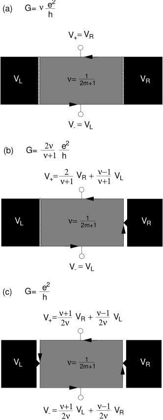
FIG. 1.: Different ways of strongly coupling a FQH liquid to reservoirs gives distinct universal values for the two-terminal conductance. In (a), the FQH liquid is coupled to the reservoirs via many contacts. The edges are in equilibrium with their respective reservoirs of departure, and the two-terminal conductance equals the Hall conductance $\nu e^{2}/h$. In (b), the left reservoir is coupled through many points, whereas the right one is coupled via a single quantum channel (one point-like contact or impurity). The electrons at the upper edge ($V_{+}$) are not in equilibrium with the right reservoir ($V_{R}$). The two-terminal conductance is $\frac{2\nu}{\nu+1}e^{2}/h$, larger than $\nu e^{2}/h$, and the Hall voltage $V_{+}-V_{-}=\frac{2}{\nu+1}(V_{R}-V_{L})>V_{R}-V_{L}$. In (c), both reservoirs are coupled via a single point-like contact. Neither branch is in equilibrium with either reservoir, and the two-terminal conductance is $e^{2}/h$, independent of the filling fraction $\nu=1/(2m+1)$.

The devices depicted in Fig 1 are particular cases of the general problem of connecting a Laughlin FQH liquid with $N_{L}$ point-contacts to the left reservoir, and $N_{R}$ point-contacts to the right one. For strong coupling (which can always be achieved for large enough voltages), we find that the universal conductance $G_{N_{L},N_{R}}$ is given by

$$G_{N_{L},N_{R}}=\frac{\left[1-\left(\frac{\nu-1}{\nu+1}\right)^{N_{L}}\right]\left[1-\left(\frac{\nu-1}{\nu+1}\right)^{N_{R}}\right]}{\left[1-\left(\frac{\nu-1}{\nu+1}\right)^{N_{L}+N_{R}}\right]}\ \nu\frac{e^{2}}{h}\ ,$$ (1)

which reproduces the cases in Fig. 1: $G_{\infty,\infty}=\nu e^{2}/h$, $G_{\infty,1}=\frac{2\nu}{\nu+1}e^{2}/h$, and $G_{1,1}=e^{2}/h$.

In this paper we also consider in detail the problem of equilibration in the presence of many impurities or contacts coupling a reservoir to the QH liquid. The case of many impurities is treated in the following way. The propagation in the reservoir side between spatially separated impurities takes place incoherently. Moreover, after scattering from a point-like contact to the QH liquid, the energy of the scattered electron would drop on the chiral Fermi branch, but would then be brought back to equilibrium with the reservoir. Thus, electrons incident into any of the impurities from the reservoir side will always be at the same voltage. On the QH liquid side, however, the energy of the scattered electron is maintained from one scattering event to another, because of the dissipationless nature of the QH state. Multi-impurity scattering will bring, eventually, the QH edge to equilibrium with the reservoir. This scattering mechanism allows one to obtain the solution of the many impurity problem from the single impurity one. Notice that the behavior of the electrons in the reservoir side, namely loss of phase memory and equilibration, is what provides the simplification needed in solving the multi-impurity case. Clearly, incoherence is a key assumption here. It must hold for well separated impurities which should act essentially independently from each other. This situation is familiar from the physics of dilute magnetic alloys where the Kondo impurities are indeed independent from each other. It is also clear that as the impurities (i. e. the contacts) become closer to each other, coherence effects in the reservoir should become important. In this limit, we expect a richer and more complex quantum behavior much like the multi-impurity or multichannel behavior in Kondo systems.

We use this framework for the multi-impurity case and apply it to obtain a solution for the case of tunneling, through many impurities, from an electron gas to a $\nu=1/3$ liquid, which is of direct relevance for comparison to the experiments of A. Chang et.  al. [5]. We show that the mechanism that we consider in this work contains the necessary ingredients to explain not only the low voltage, low temperature power law behavior, but also the breakdown voltage scale for deviations from the anomalous power law scaling. In addition, it predicts the asymptotic large voltage conductances, which should saturate at the bulk value of the Hall conductance $\nu{\frac{e^{2}}{h}}$. We show that the conductance between the electron gas and the $\nu=1/3$ FQH state is given by

$$G=\nu\frac{e^{2}}{h}\left\{1-\frac{e^{-\frac{1}{2}\left(\frac{2\pi T}{T_{K}}\right)^{2}}}{\left[\left(1-e^{-\left(\frac{2\pi T}{T_{K}}\right)^{2}}\right)\left(\frac{V}{2\pi T}\right)^{2}+1\right]^{3/2}}\right\}\ ,$$ (2)

where $T$ is the temperature and $T_{K}$ is a crossover energy scale determined by the couplings of all impurities connecting the electron gas to the QH state. The only assumption made in the derivation of Eq. (2) is that individual impurities are weakly coupled. This assumption, as we show, does not restrict the result to the regime of small conductances since the scale $T_{K}$ can actually take a broad range of values. Hence the expression should remain valid even for voltages large compared to $T_{K}$ and conductances as large as the bulk Hall value $\nu{\frac{e^{2}}{h}}$ (this point is made clear below).

The result of Eq. (2) can be used for comparison with the experimental data. One can easily check that, for $V\ll T_{K}$, Eq. (2) reproduces the scaling form used in Ref. [5]. The voltage scale for which the experimental data departs from the low voltage scaling form is determined by the energy scale $T_{K}$, which is evident in Eq.(2). This breakdown voltage scale can be determined from the low voltage data, since the amplitude of the tunneling conductance is directly related to $T_{K}$ and $T$:

$$G_{0}=\lim_{V\to 0}\ G=\nu\frac{e^{2}}{h}\left[1-e^{-\frac{1}{2}\left(\frac{2\pi T}{T_{K}}\right)^{2}}\right]\ .$$ (3)

Therefore, the “breakdown” voltage is indeed part of the full solution to the problem of tunneling into the FQH edge.

One should not overlook the fact that the experimentally measured conductance saturates to the Hall value $\nu{\frac{e^{2}}{h}}$. This is a signature of many impurities, and it is in agreement with Eq. (2). We contrast this case to the one impurity contact (to one of the reservoirs, as in Fig. 1b), for which the two-terminal conductance should reach the value $G=\frac{2\nu}{\nu+1}{\frac{e^{2}}{h}}$, and electrons enter the edge of the QH liquid hotter than the reservoir.

Finally, we would like to point out that, as a natural consequence of the physics of the point-contact junctions between bulk electron gases and FQH states that are discussed here, these junctions constitute a simple physical realization of the DC voltage transformer proposed very recently by Chklovskii and Halperin[24]. The point-contact junctions are more readily realizable and possibly avoid many of the difficulties discussed by Chklovskii and Halperin.

III Tunneling from an electron gas to a FQH edge

Our starting point is the Lagrangian density that describes the dynamics on the edge of the FQH liquid, the electron gas reservoirs, and the tunneling between the two via a single impurity:

$${\cal L}={\cal L}_{\rm edge}+{\cal L}_{\rm gas}+{\cal L}_{\rm tun}\ .$$ (4)

The edge excitations of a FQH liquid with $\nu=\frac{1}{2m+1}$ are described by a single free chiral boson field $\phi$ with

$${\cal L}_{\rm edge}={1\over 4\pi}\partial_{x}\phi(\partial_{t}-v\partial_{x})\phi$$ (5)

and equal-time commutation relation $[\phi(t,x),\phi(t,y)]=-i\pi\ {\rm sgn}(x-y)$. The edge electron operator is written in terms of the boson field as $\psi_{\rm edge}(t,x)\propto e^{-i\frac{1}{\sqrt{\nu}}\phi(t,x)}\$ [1]. ${\cal L}_{\rm gas}$ is the Lagrangian for the electron gas, with $\psi(t,x)$ the electron operator there. The tunneling Lagrangian is then

$${\cal L}_{\rm tun}=\sqrt{2\pi}\Gamma\ \delta(x)\ e^{i\omega_{J}t}\ \ e^{i\frac{1}{\sqrt{\nu}}\phi(t,0)}\psi(t,0)+H.c.\ \ .$$ (6)

The Josephson frequency $\omega_{J}=eV/\hbar$ is set by the difference of voltages between the electron gas and the incoming edge branch to the impurity. As we will see later, the voltage for the outgoing branch is raised due to tunneling.

The next step is the mapping between a 2D or 3D electron gas to a 1D chiral Fermi liquid for tunneling through a single impurity. We follow the conventional procedure used in the theory of the Kondo problem (see, for instance, Ref. [23]) where it is shown that the problem of a single isotropic magnetic impurity coupled to a three-dimensional Fermi liquid is mapped to the problem of a one-dimensional chiral Fermi liquid coupled to the impurity. The same conclusions hold for any number of dimensions greater than one. In the Kondo problem, one basically writes the electron wavefunction $\psi(\vec{r})$ in a spherically symmetric basis, with the origin at the impurity position $\vec{r}=0$. The operator $\psi(\vec{0})$ depends only on the $L=0$ harmonic, so that this is the only channel that participates in coupling to the impurity. For the case of two dimensions, only the $m=0$ channel is coupled.

One may worry that if the impurity is on the planar boundary of the 3D electron gas, the spherical symmetry is spoiled. However, the spherical symmetry is not a necessary condition to arrive at the conclusion that only one quantum channel is coupled via the impurity. We show in appendix A, for a very general set of problems, that one can always find a basis of eigenstates of the Hamiltonian for the electron gas such that only one quantum channel couples to the impurity, and again only the radial components of that channel are important. The electron operator for this channel can be written in terms of left and right moving fermions on a half line, which is the radial coordinate $r$ (left and right moving particles correspond to incoming and outgoing particles with respect to the impurity). By unfolding the half line into a full line, one can describe the electron operators in terms of a single chiral fermion on an infinite line. Therefore, for tunneling through a point-like contact, the semi-infinite 3D electron gas becomes effectively equivalent to a 1D chiral Fermi liquid. It can be regarded in much the same way as if it were a sharp edge of $\nu=1$ QH state.

Thus, we can write

$${\cal L}_{\rm gas}={\cal L}_{\rm gas}^{\bf\alpha}+{\rm other\ channels}\ ,$$ (7)

where ${\bf\alpha}$ labels the quantum numbers of the channel that couples to the impurity (which depend on the symmetry in the problem, such as $L=0$ for the Kondo problem). We can then bosonize the ${\bf\alpha}$ effective chiral 1D mode corresponding to the (unfolded) radial direction:

$${\cal L}_{\rm gas}^{\bf\alpha}={1\over 4\pi}\partial_{x}\varphi(\partial_{t}-{\tilde{v}}\partial_{x})\varphi$$ (8)

with the electron operator given (in terms of $\varphi$) by $\psi(t,x)=\frac{1}{\sqrt{2\pi}}:e^{-i\varphi(t,x)}:\$.

We are free to rescale the position coordinates and thus alter the velocities. Moreover, because the tunneling takes place at a point, and also the two chiral boson fields $\phi$ and $\varphi$ are in separate spaces, we are free to rescale the position coordinates independently, allowing us to set both $v=\tilde{v}=1$. (Notice that even though we used the same symbol $x$ for the coordinates of both fields, $x$ separately parametrizes the fields along their arc length. The only commom point in the parametrization is $x=0$, which is the impurity location.)

The tunneling problem is then described by the Lagrangian

$${\cal L} = {1\over 4\pi}\partial_{x}\phi(\partial_{t}-\partial_{x})\phi+{1\over 4\pi}\partial_{x}\varphi(\partial_{t}-\partial_{x})\varphi$$ (9)

$$\ \ \ \ +\Gamma\ \delta(x)\ e^{i\omega_{J}t}\ \ e^{i\left(\frac{1}{\sqrt{\nu}}\phi(t,0)-\varphi(t,0)\right)}+H.c.$$ (10)

We can bring the tunneling term to more familiar forms by means of a rotation. Instead of doing this directly for Eq. (9), let us treat a more general problem. Consider tunneling between a $\nu_{1}=1/n_{1}$ and a $\nu_{2}=1/n_{2}$ QH state, with both $n_{1,2}$ odd integers (single edges). The tunneling coupling is

$${\cal L}_{\rm tun} = \Gamma\ \delta(x)\ e^{i\omega_{J}t}\ \ e^{i\left(\frac{1}{\sqrt{\nu_{1}}}\phi_{1}(t,0)-\frac{1}{\sqrt{\nu_{2}}}\phi_{2}(t,0)\right)}+H.c.$$ (11)

$$= \Gamma\ \delta(x)\ e^{i\omega_{J}t}\ \ e^{i\frac{1}{\sqrt{\bar{\nu}}}\left(\phi_{a}(t,0)-\phi_{b}(t,0)\right)}+H.c.$$ (12)

where we have performed the $O(2)$ rotation

$$\left(\matrix{\phi_{a}\cr\phi_{b}}\right)=\left(\matrix{\ \cos\theta&\sin\theta\cr-\sin\theta&\cos\theta}\right)\left(\matrix{\phi_{1}\cr\phi_{2}}\right)\ ,$$ (13)

with

$$\cos\theta = \frac{1}{\sqrt{2}}\frac{\sqrt{\nu_{1}^{-1}}+\sqrt{\nu_{2}^{-1}}}{\sqrt{\nu_{1}^{-1}+\nu_{2}^{-1}}}$$ (14)

$$\sin\theta = \frac{1}{\sqrt{2}}\frac{\sqrt{\nu_{1}^{-1}}-\sqrt{\nu_{2}^{-1}}}{\sqrt{\nu_{1}^{-1}+\nu_{2}^{-1}}}\ .$$ (15)

The tunneling term corresponds to tunneling between two chiral Luttinger liquids with

$$g=\bar{\nu}^{-1}=\frac{\nu_{1}^{-1}+\nu_{2}^{-1}}{2}\ .$$ (16)

In particular, since we showed that the electron gas couples to a single impurity through only one quantum channel (see Appendix A), it is effectively equivalent to a 1D chiral Fermi liquid (virtual $\nu=1$), and so we have

$$g=\frac{\nu^{-1}+1}{2}\ ,$$ (17)

where $\nu$ is the filling fraction of the QH state coupled to the electron gas (reservoir) through the single impurity.

We can then use the known results for tunneling between two Luttinger liquids and apply to the problem of tunneling from an electron gas to the edge of a FQH liquid. We can, for example, determine the current injected into the edge branch, which depends on the voltage difference between the electron gas and the incoming branch to the impurity, as shown in Fig. 2.

Because of the weak-strong coupling duality symmetry present in the problem of tunneling between Luttinger liquids, we can also turn to the dual picture corresponding to tunneling between two Luttinger liquids with

$$\tilde{g}=\frac{1}{g}=\frac{2}{\nu^{-1}+1}\ .$$ (18)

The differential tunneling conductance depends on both $g$ (or ${\tilde{g}}$) and $V_{R}-V_{in}$. At zero temperature, it is given by [7, 8]

$$G_{t}={\tilde{g}}\ \frac{e^{2}}{h}\times\cases{\sum_{n=1}^{\infty}c_{n}(1/{\tilde{g}})\ \left(\frac{V}{2T_{K}}\right)^{2n(1/{\tilde{g}}-1)},&\mbox{$\frac{V}{2T_{K}}<e^{\delta}$}\cr 1-\sum_{n=1}^{\infty}c_{n}({\tilde{g}})\ \left(\frac{V}{2T_{K}}\right)^{2n({\tilde{g}}-1)},&\mbox{$\frac{V}{2T_{K}}>e^{\delta}$}\cr}$$ (19)

where $V$ is the voltage difference between the reservoir and the incoming edge branch, $V_{R}-V_{in}$. The $T_{K}$ is an energy scale set by the tunneling amplitude $\Gamma$ ($T_{K}\propto|\Gamma|^{-1/({\tilde{g}}^{-1}-1)}$), and the coefficients $c_{n}$ are given by

$$c_{n}({\tilde{g}})=(-1)^{n-1}\ \frac{\Gamma(n{\tilde{g}}+1)}{\Gamma(n+1)}\ \frac{\Gamma(1/2)}{\Gamma(n({\tilde{g}}-1)+1/2)}\ .$$ (20)

The domains of convergence of the dual series are restricted by $\delta=[{\tilde{g}}\ln{\tilde{g}}+(1-{\tilde{g}})\ln(1-{\tilde{g}})]/[2({\tilde{g}}-1)]$

Due to the injected current, the voltage of the edge branch past the impurity is raised by $\Delta V=I_{t}/(\nu e^{2}/h)$.

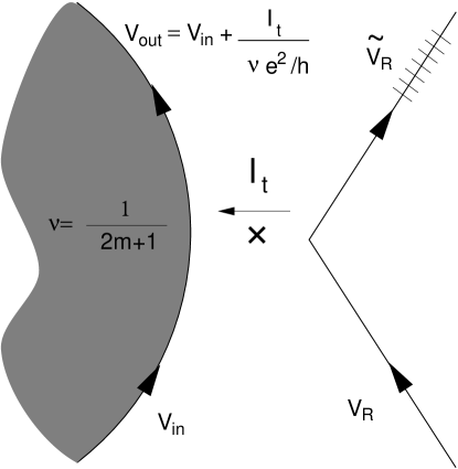
FIG. 2.: One impurity scattering picture. The only voltages that affect the tunneling current are the incoming ones, $V_{in}$ and the reservoir voltage $V_{R}$. The outgoing voltage $V_{out}$ is raised due to the injected current $I_{t}$. The outgoing voltage on the reservoir side ${\tilde{V}}_{R}$ also depends on the tunneling current; however, after scattering, electrons in this branch are equilibrated again with the reservoir.

We now turn to the case of strong coupling ($|\Gamma|\to\infty$, $T_{K}\to 0$), or equivalently, large voltage differences ($V\gg T_{K}$). In this case, the tunneling conductance reaches the strong coupling asymptotic value $G_{t}={\tilde{g}}e^{2}/h$. We then apply this result to the geometries depicted in Fig. 1.

A One point-like contact

This is the case shown in Fig. 1b. One edge branch is in equilibrium with its reservoir of departure ($V_{-}=V_{L}$), because this contact is made through many impurities (see section V). For the other contact, the value of the voltage level $V_{+}$ depends on the injected current from the right reservoir. The injected current for strong coupling is given by

$$I_{t}={\tilde{g}}\ \frac{e^{2}}{h}\ (V_{R}-V_{-})=\frac{2}{\nu^{-1}+1}\frac{e^{2}}{h}\ (V_{R}-V_{-})\ ,$$ (21)

and consequently

$$V_{+}-V_{-}=\nu^{-1}{\tilde{g}}\ (V_{R}-V_{-})=\frac{2}{\nu+1}\ (V_{R}-V_{-})\ .$$ (22)

Thus, the voltage $V_{+}$ is given by

$$V_{+}=\frac{2}{\nu+1}V_{R}\ +\ \frac{\nu-1}{\nu+1}V_{L}\ ,$$ (23)

and the Hall voltage is

$$V_{+}-V_{-}=\frac{2}{\nu+1}\ (V_{R}-V_{L})\ .$$ (24)

The two-terminal conductance of the device (determined from $I_{t}/(V_{R}-V_{L})$) is

$$G=\frac{2\nu}{\nu+1}\frac{e^{2}}{h}\ .$$ (25)

B Two point-like contacts

This is the case shown in Fig. 1c. Neither of the edge branches is in equilibrium with either reservoir. We have to determine the voltages from the tunneling currents in both contacts. The voltages $V_{+}$ and $V_{-}$ are obtained from

$$V_{+}-V_{-} = \nu^{-1}{\tilde{g}}\ (V_{R}-V_{-})=\frac{2}{\nu+1}\ (V_{R}-V_{-})$$ (26)

$$V_{-}-V_{+} = \nu^{-1}{\tilde{g}}\ (V_{L}-V_{+})=\frac{2}{\nu+1}\ (V_{L}-V_{+})\ ,$$ (27)

which give

$$V_{+} = \frac{\nu+1}{2\nu}V_{R}+\frac{\nu-1}{2\nu}V_{L}$$ (28)

$$V_{-} = \frac{\nu+1}{2\nu}V_{L}+\frac{\nu-1}{2\nu}V_{R}\ .$$ (29)

The Hall voltage is given by

$$V_{+}-V_{-}=\nu^{-1}\ (V_{R}-V_{L})\ .$$ (30)

The current flowing through the device is

$$I_{t}=\nu\frac{e^{2}}{h}\ (V_{+}-V_{-})=\frac{e^{2}}{h}\ (V_{R}-V_{L})\ ,$$ (31)

and therefore the two-terminal conductance is

$$G=\frac{e^{2}}{h}\ .$$ (32)

This result is the universal conductance for spinless non-interacting electrons. It resembles the result for the conductance of quantum wires, where the reservoirs mask the (non-chiral) Luttinger liquid behavior of the 1D wire [14, 16]. We can understand why there is such correspondence in a very simple way. Because the contacts are made to the two reservoirs at a single point each, we can deform the edges of the QH state so as to bring them to line up on top of each other at a segment that connects the two contacts. The end result is that the two opposite chiralities overlap on the same segment (see Fig. 3), which makes the problem the same as its non-chiral counterpart of Ref. [14, 16]. Notice also that we have shown that, for point-like contacts to the reservoirs, the electron gas making up the external lead behaves effectively as a 1D chiral Fermi liquid, which was the model for the leads that Maslov and Stone proposed recently[16]. In their picture, the non-chiral Luttinger liquid of a quantum wire turned adiabatically into a Fermi liquid (describing the leads) which they also took to be a one-dimensional Fermi system. Our mapping shows that only one mode of the electrons in the reservoir will effectively tunnel into the Luttinger liquid. Furthermore, even if the coupling between the leads and the wire is very smooth, there are always backscattering processes at the crossover. These processes are always relevant operators and the system always flows to strong coupling where the tunneling picture is accurate[3]. Thus, the mapping presented here provides a formal justification of the model of Maslov and Stone.

FIG. 3.: If the contacts from the FQH liquid to the reservoirs are made through a single point each, the edges can be deformed so as to line them up much in the same way as in a non-chiral Luttinger liquid (quantum wire), and so $G=e^{2}/h$. However, in contrast to quantum wires, the “extra” spatial dimension in the case of the FQH state, allows measurements (such as the ratio $\nu^{-1}$ between the Hall voltage to the two-terminal voltage), which probes the Luttinger liquid nature of the state in between the reservoirs.

Having mentioned the similarities, let us now look at the important differences between transmitting current in quantum wires and FQH liquids. The chiral 1D Luttinger liquid in the case of the FQHE comes from the edges of the 2D strongly correlated FQH liquid, and we can explore the extra one dimension experimentally. For example, one can measure voltages at the two edges ($V_{+}$ and $V_{-}$ in Fig. 1c) because they are spatially separated, and by doing so probe Luttinger liquid behavior between the reservoirs. This is not possible in the case of quantum wires, for the two chiralities are mixed and one cannot measure the two chemical potentials separately inside the wire. A measurement of the Hall voltage $V_{+}-V_{-}=\nu^{-1}(V_{R}-V_{L})$ returns a value that is larger than the two-terminal voltage ($V_{R}-V_{L}$) by a factor of $\nu^{-1}$; this factor contains information on the Luttinger liquid behavior between the reservoirs which is experimentally measurable, and has no counterpart in quantum wires.

Another important difference between quantum wires and devices such as the ones we discuss in this paper is that quantum wires can be connected to leads in only one way (i. e., one end to each lead), whereas we can connect a FQH state (a 2D system) to, say, $N_{L}$ contacts to one reservoir and $N_{R}$ to the other. The consequence is that in quantum wires one can only observe a conductance $e^{2}/h$ (and multiples of it), whereas for FQH states the conductance $G_{N_{L},N_{R}}$, as we show in section V, can take values in whole families of rational multiples of $e^{2}/h$. (Examples are the cases shown in Figs. 1b and 1c, which correspond to $G_{\infty,\infty}=\nu e^{2}/h$ and $G_{\infty,1}=\frac{2\nu}{\nu+1}e^{2}/h$, respectively.)

In summary, the strong coupling (large voltage) value of the tunneling conductance from a reservoir ( i. e. , a Fermi liquid) to the chiral Luttinger liquids of the edges of a FQH state, in spite of being universal, depends not only on the properties of the FQH liquid but also on the nature of the contacts. Moreover, the physics of the edge states of the FQH states can be probed with a variety of junctions for which there is no counterpart in one-dimensional quantum wires.

IV Experimental realization of g=1/2

A very interesting case is when $\nu=1/3$, in which case $g=2$. This case is the dual point to ${\tilde{g}}=1/2$, which is exactly solvable, not only for the conductance, but for the full noise spectrum (indeed, all $n$-point correlation functions). This non-trivial exactly solvable point is very important theoretically because it provides the comparison ground for any result obtained perturbatively. Before, it was simply a theoretical tool, with no physical realization. The tunneling from an electron gas to a $\nu=1/3$ state makes it now possible to study the important $g=1/2$ state experimentally.

Let us focus on this $g=1/2$ case and a single impurity. The exact solution (see Refs.[3, 7, 10] and references therein) for the tunneling current and differential conductance is

$$I_{t} = e\int\frac{d\omega}{2\pi}\ \frac{\omega^{2}}{\omega^{2}+(T_{K}/2)^{2}}\ \left(f(\omega-\omega_{0})-f(\omega)\right)$$ (33)

$$G_{t} = \frac{1}{2}\frac{e^{2}}{h}\int d\omega\ \frac{\omega^{2}}{\omega^{2}+(T_{K}/2)^{2}}\ \left(-f^{\prime}(\omega-\omega_{0})\right)\ ,$$ (34)

where $f=(1+e^{\omega/T})^{-1}$ is the Fermi distribution, $\omega_{0}=\frac{1}{2}\frac{eV}{\hbar}$, and $T_{K}=(2\pi|\Gamma|)^{-1}$. The $\omega_{0}$ and $T_{K}$ are, besides the temperature, the two energy scales in the problem. As one varies the voltage, the current and conductance scaling with $V$ changes depending on the relative value of $V$ as compared to $T$ and $T_{K}$. Consider, for example, the case when $T\ll T_{K}$. In this case, the conductance scales as

$$G_{t}\approx\ \frac{1}{2}\frac{e^{2}}{h}\cases{\frac{1}{3}\left(\frac{2\pi T}{T_{K}}\right)^{2},&\mbox{$V\ll T$}\cr\ \ \left(\frac{V}{T_{K}}\right)^{2}\ \ \ ,&\mbox{$T\ll V\ll T_{K}$}\cr\ \ \ \ 1\ \ \ \ \ \ \ ,&\mbox{$V\gg T_{K}$}\cr}\ .$$ (35)

The anomalous scaling of the current with voltage that is characteristic of Luttinger liquids takes place between the two energy scales $T$ and $T_{K}$. In recent experiments, Chang et. al. have observed such scaling. In the experimental data, the $G_{t}\propto V^{\alpha}$ power law scaling breaks down at a certain voltage. One is inclined to think that $T_{K}$ provides the energy scale for the breakdown, although in that particular experiment tunneling takes place not through one, but many impurities. The idea that there is another energy scale in the problem, however, is still an important one, and we will show that indeed such a breakdown scale also occur for the many impurity problem.

V Multiple impurities and Equilibration

We will here show how to treat the problem of tunneling from an electron gas or reservoir to a QH liquid via many impurities. In the previous section we considered scattering through a single impurity (see Fig. 2), in which case the incident edge channel comes at a voltage level $V_{in}$, and the electron from the reservoir at $V_{R}$. After scattering, the edge is at $V_{out}$, and the reservoir branch at ${\tilde{V}}_{R}$. We will obtain the many impurity result by considering the single scattering event as building blocks, and cascading them.

An important issue for this cascading is that of how the scattered electrons on the reservoir side behave differently from those in the QH side in between scattering events. In the reservoir side, regardless of the voltage after scattering, the electrons will equilibrate with the reservoir by the time of the next scattering event. It will also lose its phase memory. This means that on the reservoir side, electrons will always arrive for the scattering events at the same voltage, namely, $V_{R}$. On the QH side, however, the voltage is maintained between scattering events, and is accumulated. Thus, the cascade can be assembled as shown in Fig. 4.

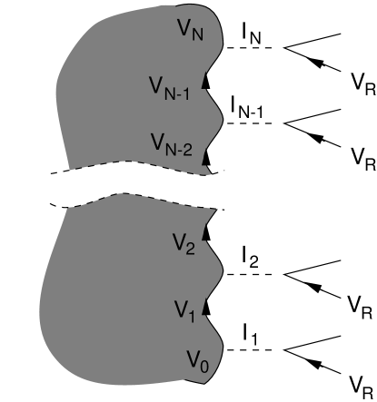
FIG. 4.: Multi ($N$) impurity scattering, assembled from the one impurity building block. Notice that the voltages on the FQH liquid side are maintained in between scattering events, whereas on the reservoir side electrons come for the scattering always at $V_{R}$.

The voltages past the $n$-th stage of the cascade are labeled $V_{n}$, and the current flowing from the reservoir to the QH liquid is $I_{n}$. The voltage difference between the outgoing ($V_{n}$) and incoming ($V_{n-1}$) edge states is obtained from the current $I_{n}$ and the Hall conductance for the QH liquid:

$$V_{n}-V_{n-1}=\frac{I_{n}}{\nu\frac{e^{2}}{h}}\ .$$ (36)

Now, the current $I_{n}$ is simply the single impurity tunneling current, which depends on the incoming state ($n-1$) and the coupling strength for the $n$-th impurity, as well as the temperature. The coupling strength enters as an effective temperature $T_{K}^{(n)}$ for a given impurity.

Notice, however, that the voltages $V_{n}$ alone are not sufficient to describe the quantum states at the different stages of the cascade. One needs the states $|\Phi_{n}\rangle=|V_{n};\{n_{k}\}_{n}\rangle$, where the $n_{k}$ are the occupation numbers of the oscillator modes of the chiral boson $\phi$ describing the edge state. The voltage $V_{n}$ measures the total charge or the zero mode of the boson field. The non-zero modes should in principle affect the $I-V$ characteristics for each impurity. An intuitive picture one can use to see the effects of the excited oscillator modes is that they could account for an “effective” increase in the temperature (since a higher temperature brings more excited modes). This “effective” increase in the temperature enters in the expression for the tunneling current, in addition to the voltages $V_{n}$ and $V_{R}$.

Nonetheless, there are two regimes where the oscillator modes are not excited: weak and strong coupling. Effects due to the oscillator modes, as described above, become only important at intermediate coupling. For the weak and strong coupling cases we can simply use the $I-V$ characteristics for a single impurity to obtain recursively the voltages $V_{n}$ for all $n$, and we can obtain the total current that flows to the QH liquid from $I=\nu\frac{e^{2}}{h}(V_{N}-V_{0})$, where $N$ is the last impurity on the line, and $V_{0}$ is the initial voltage level of the edge (in equilibrium with the other reservoir). The recursion equation is

$$V_{n}-V_{n-1}=\frac{1}{\nu e^{2}/h}\ I_{t}(V_{R}-V_{n-1},T_{K}^{(n)},T)\ .$$ (37)

Let us study solutions of these recursion relations for different regimes of tunneling strengths.

A Weak coupling

Without loss of generality, let us concentrate on the case $g=2={\tilde{g}}^{-1}$. We will not use the fact that ${\tilde{g}}=1/2$ is exactly solvable; we just choose this example for clarity of presentation, and because it is applicable to tunneling from an electron gas to a $\nu=1/3$ FQH state. (We will present the result for general $g$ after the derivation for $g=2={\tilde{g}}^{-1}$).

If the individual couplings are small, the $T_{K}^{(n)}$ will be large, in which case we can use for the individual impurities the low voltage ($V\ll T_{K}^{(n)}$) expression for the current:

$$I_{n}=\frac{e^{2}}{h}\frac{T_{K}^{(n)}}{6}\left(\frac{2\pi T}{T_{K}^{(n)}}\right)^{3}\left[\frac{V_{R}-V_{n-1}}{2\pi T}+\left(\frac{V_{R}-V_{n-1}}{2\pi T}\right)^{3}\right]\ .$$ (38)

Now, we let $x_{n}=\frac{V_{R}-V_{n}}{2\pi T}$ and substitute it into the recursion relation Eq. (37), obtaining

$$x_{n}-x_{n-1}=-\frac{1}{6\nu}\left(\frac{2\pi T}{T_{K}^{(n)}}\right)^{2}\ (x_{n-1}+x_{n-1}^{3})\ ,$$ (39)

which we can transform into a differential equation, since the couplings are assumed to be small:

$$\frac{dx}{dn}=-\frac{1}{6\nu}\left(\frac{2\pi T}{T_{K}^{(n)}}\right)^{2}\ (x+x^{3})\ ,$$ (40)

to be integrated from the initial $x_{0}$ to the final $x_{N}$ (past the last impurity $N$) yielding

$$\int_{x_{0}}^{x_{N}}\frac{dx}{x+x^{3}}=-\sum_{n=1}^{N}\frac{1}{6\nu}\left(\frac{2\pi T}{T_{K}^{(n)}}\right)^{2}=-\frac{1}{2}\left(\frac{2\pi T}{T_{K}}\right)^{2}\ ,$$ (41)

in which we define the effective $T_{K}$ from the individual $T_{K}^{(n)}$. A very important point to be noticed is that one needs not assume that the couplings $T_{K}^{(n)}$ are uniform; they can fluctuate, and the only important parameter is the effective $T_{K}$ which incorporates even the fluctuations. After integration, one obtains

$$\frac{x_{N}}{\sqrt{1+x_{N}^{2}}}=e^{-\frac{1}{2}\left(\frac{2\pi T}{T_{K}}\right)^{2}}\frac{x_{0}}{\sqrt{1+x_{0}^{2}}}\ ,$$ (42)

or equivalently,

$$V_{N}=V_{R}-2\pi T\left\{e^{\left(\frac{2\pi T}{T_{K}}\right)^{2}}\left[1+\left(\frac{V}{2\pi T}\right)^{-2}\right]-1\right\}^{-1/2}\ ,$$ (43)

where $V=V_{R}-V_{L}$. We have used that $x_{0}=\frac{V}{2\pi T}$, taking the incoming edge at equilibrium with the other reservoir ($V_{0}=V_{L}$). The total current flowing to the QH liquid is obtained from the voltage difference $V_{N}-V_{0}$, and is given by $I=\nu\frac{e^{2}}{h}(V_{N}-V_{0})$. The differential conductance then yields

  

$$G=\nu\frac{e^{2}}{h}\left\{1-\frac{e^{-\frac{1}{2}\left(\frac{2\pi T}{T_{K}}\right)^{2}}}{\left[\left(1-e^{-\left(\frac{2\pi T}{T_{K}}\right)^{2}}\right)\left(\frac{V}{2\pi T}\right)^{2}+1\right]^{3/2}}\right\}\ .$$ (44)

The derivation for general $g$ is similar, and gives

$$G=\nu\frac{e^{2}}{h}\left\{1-\frac{e^{-\frac{1}{2}\left(\frac{2\pi T}{T_{K}}\right)^{2(g-1)}}}{\left[\frac{1}{\Gamma^{2}(g)}\left(1-e^{-(g-1)\left(\frac{2\pi T}{T_{K}}\right)^{2(g-1)}}\right)\left(\frac{V}{2\pi T}\right)^{2(g-1)}+1\right]^{\frac{2g-1}{2(g-1)}}}\right\}\ .$$ (45)

   

The result expressed in equation (44) holds for all values of $V,T,T_{K}$, as long as the assumptions used to derive the expression holds, namely, that each individual impurity is weakly coupled. Notice that, even though the $T_{K}^{(n)}$ are large, the effective $T_{K}$ for the the line of impurities can be made small by simply having a very long line (large $N$). Experimentally one has two ways of varying $T_{K}$: changing the tunneling barriers, and taking wider samples.

We can use Eq. (44) for comparison with recent experiments by A. Chang et.al. [5]. The experiments demonstrate power law scaling of the tunneling current with voltage. For small voltages, the data is well fitted by a universal $I-V$ characteristic which crosses over from a linear regime for $V\ll T$, to the power law scaling for $V\gg T$. One can easily check that the universal curve used for the conductance correspond to the $T,V\ll T_{K}$ limit of Eq. (44), namely

$$G\approx\nu\frac{e^{2}}{h}\frac{1}{2}\left(\frac{2\pi T}{T_{K}}\right)^{2}\left[1+3\left(\frac{V}{2\pi T}\right)^{2}\right]\ .$$ (46)

However, the fit used in Ref. [5] breaks down beyond a certain voltage scale. This suggests that there should be another energy scale in the problem which was not considered. This scale, we argue in this paper, is simply $T_{K}$. In fact, notice that one can determine $T_{K}$ from the low voltage data, as the amplitude of the tunneling conductance (which in Ref. [5] was a fitting parameter) is directly related to $T_{K}$ and the measured temperature $T$:

$$G_{0}=\lim_{V\to 0}\ G=\nu\frac{e^{2}}{h}\left[1-e^{-\frac{1}{2}\left(\frac{2\pi T}{T_{K}}\right)^{2}}\right]\ .$$ (47)

In the case of the data in Ref. [5], $G_{0}\ll\nu e^{2}/h$, in which case $T_{K}$ must be larger than the temperature scale, and $G_{0}\approx\nu\frac{e^{2}}{h}{\frac{1}{2}\left(\frac{2\pi T}{T_{K}}\right)^{2}}$. The same value of $T_{K}$ which is determined from the low voltage data ($V\ll T)$ determines the energy scale for the breakdown of the scaling form used in the fitting of the experimental data. The breakdown voltage is $V\approx T_{K}$, and is taken into account in Eq. (44), which holds for the full range of probed voltages.

The scaling form used in Ref. [5] should break down when the conductance becomes comparable to the natural conductance scale in the problem, $\nu{\frac{e^{2}}{h}}$. This is explicit in Eq. (44). One should also interpret with care the fact that the conductance saturates to the Hall value $\nu{\frac{e^{2}}{h}}$. This is a point which should be taken into account carefully, since for tunneling through a single impurity, as seen in the previous section, the asymptotic value should be $\frac{2\nu}{\nu+1}{\frac{e^{2}}{h}}>\nu{\frac{e^{2}}{h}}$. What this says is that for a small tunneling conductance, the multi-impurity problem is very much like the single impurity one, but for large tunneling conductance there must be a mechanism that lowers the asymptotic value of the conductance to $\nu{\frac{e^{2}}{h}}$. This mechanism is brought about by the multiple impurities.

In Figures 5 and 6 we show, for $\nu=1/3$ in two different samples, the comparison between the experimental data for the conductance and the scaling form of Eqs. (44) and (45), valid for the full range of probed voltages. We obtain the ratio $T_{K}/T$ from the asymptotic low voltage conductance. For the data set of Fig. 5 we use a temperature of $T=25mK$, the quoted experimental value. However, the data of Fig. 6 appears to be consistent with a higher temperature, close to $T=35mK$, rather than $25mK$. We would like to point out that our Eq. 46, which is a low voltage approximation of the full scaling form of the conductance of Eq. 44, is the same as the one used to fit the data in ref. [5] with an exponent $\alpha=2g-1$.

The theoretical curve for $g=2$ (Eq. (44) (or $\alpha=2g-1=3$) fits well the low-voltage data points, has a high voltage crossover at about the right scale ($T_{K}$), and saturates to the right high voltage asymptotic value ($\nu e^{2}/h$). However, for both samples, it seems to overshoot the experimental data just above the crossover energy scale. Instead, if we use Eq. (45) with an effective exponent of $g=1.8$ ($\alpha=2g-1=2.6$), we get a better fit to the data set over the full range of voltages. Notice, however, that the value of $T_{K}$ for the two scaling forms changes by about a factor of $2$ (for both samples).

The question on whether the exponent $g$ can be modified is an important issue. In the case of tunneling from an electron gas into a single chiral edge, the exponent cannot be modified since it is determined by the dimension of the leading irrelevant operator and should be $g=2$ ($\alpha=3$) for $\nu=1/3$. An effective exponent $\alpha\not=3$ is indicative that there is an additional crossover in the physics of these junctions. A related issue is that if we use $\alpha=3$, we find that the data is best fitted with values of $T_{K}$ which are approximately half of those obtained for $\alpha\approx 2.6$. This is a rather large change. A possible explanation is that subleading irrelevant tunneling operators are also coupled. The main effects of such operators is to alter the corrections to scaling. For example, the leading irrelevant operators cause an effective $V$ dependence in the Kondo like temperature scale $T_{K}$. In this case Eq. (44), which assumes a $T_{K}$ that does not scale, should be modified accordingly. Such a $V$ dependent correction to $T_{K}$ could be a reason why other values of $g$ and Eq. (45) fit the experimental data better. However, other scenarios are also possible. For instance, if there is clustering of tunneling centers at the atomic scale, the effective Hamiltonian will involve more that one impurity and more than one channel of the electron gas. If that were the case, there would be additional multi-impurity/multi-channel crossovers just above the Kondo scale but will not affect neither the low voltage regime nor the high voltage regime.

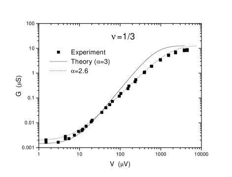
FIG. 5.: Comparison between experimental and theoretical conductances for tunneling between an electron gas and a $\nu=1/3$ FQH state - data set #1. The values $T=25mK$ (in agreement with the measured value) and $T_{K}=11K$ used in the theoretical ($g=2$, $\alpha=2g-1=3$) plots are chosen to fit the low voltage end of the curve. A better fit to the data is achieved using Eq. (38) with $g=1.8$ (or $\alpha=2g-1=2.6$), $T=25mK$ and $T_{K}=26.1K$. (Experimental data is courtesy of A. Chang.)

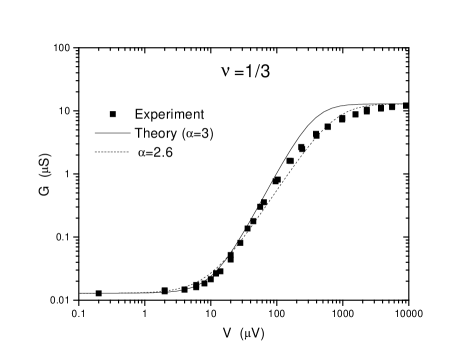
FIG. 6.: Comparison between experimental and theoretical conductances for tunneling between an electron gas and a $\nu=1/3$ FQH state - data set #2. The set is best fit with a temperature $T=35mK$, higher than the quoted $T=25mK$. The values of $T_{K}$ are $4.9K$ for the theoretical ($g=2$, $\alpha=2g-1=3$) curve, and $10.7K$ for the fit achieved using Eq. (38) with $g=1.8$ (or $\alpha=2g-1=2.6$). In this set there are more high voltage data points, which allows one to see that the measured conductance saturates at $G=\frac{1}{3}e^{2}/h$, in agreement with the theoretical prediction for multi-impurity tunneling. This case is to be contrasted to the single impurity value $G=\frac{1}{2}e^{2}/h$. (Experimental data is courtesy of A. Chang.)

B Strong coupling

Now let us discuss the case where the individual impurity couplings are strong. In this case, we can still use the same recursion Eq. (37) with the strong coupling or high voltage ($V\gg T_{K}^{(n)}$) expression for the current. Notice that what defines the strong coupling regime is the ratio between the voltages and the energy scales set by the impurities ($T_{K}^{(n)}$). Thus, for large enough voltages, tunneling proceeds as if the coupling were strong, even if the nominal coupling constants are finite. In this regime, for each individual impurity, the conductance saturates at the value ${\tilde{g}}\frac{e^{2}}{h}=\frac{2\nu}{\nu+1}\frac{e^{2}}{h}$, so that we have a recursion

$$V_{n}-V_{n-1} = \nu^{-1}{\tilde{g}}\ (V_{R}-V_{n-1})$$ (48)

$$= \frac{2}{\nu+1}\ (V_{R}-V_{n-1})\ ,$$ (49)

which has a solution

$$V_{n}=V_{L}+(V_{R}-V_{L})\left[1-\left(\frac{\nu-1}{\nu+1}\right)^{n}\right]\ .$$ (50)

Again, we have used that $V_{0}=V_{L}$ is the voltage at the incoming edge branch, which is equilibrium with the other reservoir. Notice that the voltage after scattering through the $n$-th impurity converges to $V_{\infty}=V_{R}$, but not monotonically, oscillating around the asymptotic value (because the argument being raised to the power $n$ is negative, since we have $\nu<1$). For example, in the case of $\nu=1/3$, the sequence of voltages $(V_{n}-V_{L})/(V_{R}-V_{L})$ is $\{0,3/2,3/4,9/8,15/16,\dots\}$, where we recognize $V_{1}$ as the strong coupling result from the single impurity problem.

The conductance can be obtained from the current through the device, $I=\nu(e^{2}/h)\ (V_{N}-V_{0})$, which yields

$$G_{N}=\nu\left[1-\left(\frac{\nu-1}{\nu+1}\right)^{N}\right]\ \frac{e^{2}}{h}\ .$$ (51)

We thus have a sequence of quantized conductances converging to the Hall value $\nu e^{2}/h$. For example, for $\nu=1/3$ the sequence is

$$G_{N}=\left\{\frac{1}{2},\frac{1}{4},\frac{3}{8},\frac{5}{16},\dots,\frac{1}{3}\right\}\frac{e^{2}}{h}\ ,$$ (52)

and for $\nu=1/5$

$$G_{N}=\left\{\frac{1}{3},\frac{1}{9},\frac{7}{27},\frac{13}{81},\dots,\frac{1}{5}\right\}\frac{e^{2}}{h}\ .$$ (53)

For $\nu=1$ we have the uninteresting and expected result that all $G_{N}=e^{2}/h$, for all $N$.

In the above, we have assumed that the contact with the left reservoir is made through many impurities, so that $V_{0}=V_{L}$. One can easily treat in a very similar manner the case of $N_{L}$ contacts with the left reservoirs, and $N_{R}$ contacts with the right one (as we did the case of one contact for each in section III). This general case will display a conductance $G_{N_{L},N_{R}}$ which will depend on both $N_{L}$ and $N_{R}$:

$$G_{N_{L},N_{R}}=\frac{\left[1-\left(\frac{\nu-1}{\nu+1}\right)^{N_{L}}\right]\left[1-\left(\frac{\nu-1}{\nu+1}\right)^{N_{R}}\right]}{\left[1-\left(\frac{\nu-1}{\nu+1}\right)^{N_{L}+N_{R}}\right]}\ \nu\frac{e^{2}}{h}\ .$$ (54)

One can check that this formula, in particular, reproduces the cases in Fig. 1: $G_{\infty,\infty}=\nu e^{2}/h$, $G_{\infty,1}=\frac{2\nu}{\nu+1}e^{2}/h$, and $G_{1,1}=e^{2}/h$.

C Large number of impurities and equilibration

One common conclusion to the case of weakly or strongly coupled individual impurities is that, for a large number of them, the outgoing edge equilibrates with the reservoir. How the series $V_{n}$ reaches the asymptotic value $V_{R}$ may vary, but if the series converge, it must converge to $V_{R}$ for a large number of impurities $N$. Indeed, this result is a statement that the attractor for the recursion relation Eq. (37) is a single fixed point. The recursion Eq. (37) implies that, if the voltages $V_{n}$ converge, then $V_{\infty}=V_{R}$, independent of the impurity couplings.

This is the mechanism for equilibration between the edge and the reservoir. It had been noticed by Kane and Fisher that impurity tunneling was key in this equilibration, in the case where one can assume that the effect of tunneling is a small leaking conductance which would equilibrate the edge and reservoir past an equilibration length dependent on the leak conductance. What we show here is that this equilibration mechanism is sturdier and more complex, equilibrating edge and reservoir for very general coupling distributions. The most striking example is that of strong coupling, where the asymptotic voltage is reached non-monotonically, which is important to understand how the result of a single impurity (hot electrons) is possible, and can be reconciled with the idea of tunneling causing equilibration.

VI Conclusions

In this paper we have investigated the problem of tunneling from an electron gas (reservoir) to a FQH state for different types of contacts. We showed that different universal values can be obtained for the two-terminal conductance. At large voltages, or strong coupling, the conductance of a point-like tunneling junction between an electron gas reservoir and a Laughlin FQH state at filling fraction $\nu$ was shown to saturate to a universal value $G={\frac{2\nu}{\nu+1}}{\frac{e^{2}}{h}}$. We used this result to show that devices with different types of contacts between the reservoir and the FQH state lead to distinct universal values of saturation conductance which are rational multiples of $e^{2}/h$. In particular, the fraction $e^{2}/h$ was obtained for the case of electron tunneling in and out of a FQH liquid by two point contacts. We demonstrated that the problem of tunneling between an electron gas and a fractional quantum Hall state through an impurity is exactly equivalent to the problem of tunneling between a chiral Fermi liquid and a chiral Luttinger liquid. The interesting case of tunneling to a $\nu=1/3$ FQH state was investigated in detailed and shown to be equivalent to the problem of tunneling between two $g=1/2$ chiral Luttinger liquids. This system provides an experimental realization of this important exactly solvable case. The results of the single impurity problem were used to consider the case of many tunneling centers coupled independently to an electron reservoir. This problem is relevant to recent experiments by A. Chang et. al. Using the exact solution of the single impurity problem, we derived an explicit universal expression for the voltage and temperature dependent conductance for a problem of many independent impurities. Here we made the key assumption that the channels of the electron gas which couple to each individual impurity are always in equlibrium or, what is the same, that there is no phase coherence between channels. This assumption must be accurate for widely separated tunneling impurities of an atomically smooth junction. We showed that the voltage and temperature dependent conductance exhibits a crossover reminiscent of a Kondo effect with a Kondo scale $T_{K}$ determined by the tunneling matrix matrix element. This universal curve was shown to fit the experimental data over the full range of probed voltages. It was also observed that this universal curve oveshoots the experimental data on a voltage scale above $T_{K}$ but below saturation where an effective exponent was found to give a better fit to the data. We interpreted this effective exponent as indicating that either a subleading irrelevant operator had a significant amplitude (which would be the case if the edge structure is not sharp) or that the physical samples had some degree of clustering of tunneling centers, leading to multi-channel/multi-impurity physics. Also, in this work we have assumed that the tunneling matrix element $\Gamma$ is independent of the applied voltage. Clearly, as $V$ increases $\Gamma$ should change [25]. However, these changes amount to an analytic redefinition of the coupling constant and are non-universal. Such effects lead to a redefinition of $T_{K}$, and do not change either the exponent or the saturation conductance.

ACKNOWLEDGEMENTS

We are particularly grateful to Albert Chang for several enlightening discussions, as well as for making his data available to us. We would also like to thank Matthew Grayson and Nancy Sandler for many useful comments. This work was supported in part by the National Science Foundation through the grants NSF DMR94-24511 at the University of Illinois at Urbana-Champaign and NSF DMR-89-20538 at the Materials Research Laboratory of the University of Illinois at Urbana-Champaign.

A General map from a high dimensional electron gas to a 1D chiral Fermi liquid for tunneling through a single impurity

Here we consider in detail the general problem of coupling an impurity to an electron gas subject to generic boundary conditions. We show that, regardless of details of the boundary conditions, only one quantum channel couples to the impurity, and the electron gas can be regarded as a 1D chiral Fermi liquid as what concerns the impurity coupling.

The sufficient assumption that we make is that the electron gas in the bulk is isotropic, so that the energy $\epsilon({\vec{k}})$ of the bulk eigenstates depends only on $|{\vec{k}}|$. In this case we can expand the electron operator as

$$\psi(\vec{x})=\int_{0}^{\infty}dk\sum_{\bf\lambda}\ \phi_{k,{\bf\lambda}}(\vec{x})\ c_{\bf\lambda}(k)\ ,$$ (A1)

where $\{\phi_{k,{\bf\lambda}}(\vec{x})\}$ is a complete set on one-particle eigenstates which satisfy the correct boundary conditions. Here $\{{\bf\lambda}\}$ is a set of quantum numbers which label degenerate states with the same wavenumber $k$ and $\epsilon(k)$. The electron operator obey the anti-commutation relation

$$\{c^{\dagger}_{\bf\lambda}(k),c_{\bf\lambda^{\prime}}(k^{\prime})\}=\delta_{{\bf\lambda},{\bf\lambda^{\prime}}}\ \delta(k-k^{\prime})\ .$$ (A2)

At the impurity location, which we take to be ${\vec{x}}=0$, we have

$$\psi(0)=\int_{0}^{\infty}dk\sum_{\bf\lambda}\ \phi_{k,{\bf\lambda}}(0)\ c_{\bf\lambda}(k)\ ,$$ (A3)

and because the states with the same $k$ are degenerate, we can perform an orthonormal transformation so as go to a new basis where

$${\tilde{c}}_{\bf\alpha}(k)={\frac{1}{{\cal N}_{k}}}\sum_{\bf\lambda}\ \phi_{k,{\bf\lambda}}(0)\ c_{\bf\lambda}(k)$$ (A4)

is a basis vector. The normalization factor ${\cal N}_{k}$ appears because the vector has not necessarily norm 1 ($\psi(0)$ has weight at different $k$). This can always be done via a Gram-Schmidt orthogonalization process. Notice that the fact that there is a single impurity is used here: one impurity picks only one direction in each subspace labelled by $k$. Hence, we can always use this one direction as the first basis vector in the Gram-Schmidt process.

We can thus write

$$\psi(0)=\int_{0}^{\infty}dk\ {\cal N}_{k}\ {\tilde{c}}_{\bf\alpha}(k)\ ,$$ (A5)

which displays clearly that the impurity only couples to a single channel (${\bf\alpha}$). The fermion operators in this channel satisfy $\{{\tilde{c}}^{\dagger}_{\bf\alpha}(k),{\tilde{c}}_{\bf\alpha}(k^{\prime})\}=\ \delta(k-k^{\prime})$.

The coupled (${\bf\alpha}$) channel can be described in terms of non-chiral fermions in a semi-infinite line, where left and right moving particles correspond to incoming and outgoing particles with respect to the impurity. This half-line can be unfolded, so we are left with one chiral fermion on an infinite line. Thus, from the perspective of the impurity, the electron gas can be regarded as a chiral Fermi liquid. One should notice that $g=1$ is completely fixed in this problem, because the chiral fermions are derived from a higher dimensional system, where the Fermi liquid picture holds.

Below we give particular examples which are applications of our general result.

1 Spherically symmetric system

This case is a simple application of the general result. Here we follow closely the derivation for the case of the impurity at the bulk by Affleck and Ludwig [23].

In this case, one writes the electron operator in terms of plane waves as

$$\psi(\vec{x})=\int\frac{d^{3}k}{(2\pi)^{3/2}}\ e^{i\vec{k}\cdot\vec{x}}\ c_{\vec{k}}\ ,$$ (A6)

where the operators $c_{\vec{k}}$ satisfy the anti-commutation relations $\{c^{\dagger}_{\vec{k}},c_{\vec{k}^{\prime}}\}=\delta^{3}({\vec{k}}-{\vec{k}^{\prime}})$. One then notices that at the impurity location $\vec{x}=0$,

$$\psi(0)=\int\frac{d^{3}k}{(2\pi)^{3/2}}\ c_{\vec{k}}$$ (A7)

depends only on the spherically symmetric component ($L=0$) of the operator $c_{\vec{k}}$, namely

$$c_{L=0}(k)=\frac{k}{\sqrt{4\pi}}\int d\hat{\Omega}\ c_{\hat{\Omega}k}\ ,$$ (A8)

which satisfy $\{c^{\dagger}_{L=0}(k),c_{L=0}(k^{\prime})\}=\delta(k-k^{\prime})$. Thus, one has only to consider the 1-D fermions running along the radial coordinates for the $L=0$ mode for the purposes of coupling to the impurity at $\vec{x}=0$.

2 Impurity at a planar boundary of a 3D electron gas

we now consider in detail the case when the point-like contact or impurity is not in the bulk, but at the planar boundary between a free electron gas and a potential barrier that confines the gas. Here we have to take into account that the eigenstates are modified by the presence of the boundary.

Let the boundary be at the $z=0$ plane. Let the barrier high be $U>0$ for $z<0$, and 0 for $z>0$. The effect of the barrier on the wavefunctions can be absorbed completely in the phase shift that the electron picks up after reflecting of the boundary (the barrier is confining, so the Fermi level lies under the barrier height, and thus the barrier is completely reflecting). The wavefunctions for $z>0$ can then be written as

$$\phi^{(+)}_{{\vec{k}}_{\perp},k_{z}}(\vec{x})=e^{i{\vec{k}}_{\perp}\cdot x_{\perp}}\ \frac{e^{-i\frac{1}{2}\phi(k_{z})}\ e^{ik_{z}z}+e^{i\frac{1}{2}\phi(k_{z})}\ e^{-ik_{z}z}}{\sqrt{2}}\ ,$$ (A9)

where $e^{i\phi(k_{z})}$ is the phase shift factor due to the reflection at the boundary of a wave with momentum $k_{z}$ (notice that $\phi(k_{z})=-\phi(-k_{z})$). It is an elementary exercise to show that for a potential barrier of of height $V$ the phase shift is given by $\cos(\phi(k_{z})/2)=|{k_{z}}/{k_{0}}|$, where $k_{0}=\sqrt{2mU}/\hbar$.

The operator that creates the state $\phi^{(+)}_{{\vec{k}}_{\perp},k_{z}}(\vec{x})$ can be written in terms of plane wave creation operators $c^{\dagger}_{\vec{k}}$ as

$${\gamma^{(+)}}^{\dagger}_{{\vec{k}}_{\perp},k_{z}}=\frac{e^{-i\frac{1}{2}\phi(k_{z})}\ c^{\dagger}_{{\vec{k}}_{\perp},k_{z}}+e^{i\frac{1}{2}\phi(k_{z})}\ c^{\dagger}_{{\vec{k}}_{\perp},-k_{z}}}{\sqrt{2}}\ .$$ (A10)

Although the general result we have shown has a simple proof, the aplication to a particular case involves explicitly finding the right basis. In this particular problem at hand, this can be greatly simplified by exploring symmetries and enlarging the Hilbert space.

The operators ${\gamma^{(+)}}^{\dagger}_{{\vec{k}}_{\perp},k_{z}}$ generate only half the Hilbert space for free fermions without the boundary. The other half is generated from wavefunctions of different symmetry

$$\phi^{(-)}_{{\vec{k}}_{\perp},k_{z}}(\vec{x})=e^{i{\vec{k}}_{\perp}\cdot x_{\perp}}\ \frac{e^{-i\frac{1}{2}\phi(k_{z})}\ e^{ik_{z}z}-e^{i\frac{1}{2}\phi(k_{z})}\ e^{-ik_{z}z}}{\sqrt{2}}\ ,$$ (A11)

by operators

$${\gamma^{(-)}}^{\dagger}_{{\vec{k}}_{\perp},k_{z}}=\frac{e^{-i\frac{1}{2}\phi(k_{z})}\ c^{\dagger}_{{\vec{k}}_{\perp},k_{z}}-e^{i\frac{1}{2}\phi(k_{z})}\ c^{\dagger}_{{\vec{k}}_{\perp},-k_{z}}}{\sqrt{2}}\ .$$ (A12)

We can redefine fermion operators ${\tilde{c}}_{\vec{k}}={\rm sgn}(k_{z})\ e^{i\frac{1}{2}\phi(k_{z})}\ c_{\vec{k}}$ so as absorb the phases into the free fermions. The Hamiltonian for the system is just that for free fermions $c_{\vec{k}}$:

$$H=\int\frac{d^{3}k}{(2\pi)^{3/2}}\ \frac{\hbar^{2}k^{2}}{2m}\ c^{\dagger}_{\vec{k}}c_{\vec{k}}=\int\frac{d^{3}k}{(2\pi)^{3/2}}\ \frac{\hbar^{2}k^{2}}{2m}\ {\tilde{c}}^{\dagger}_{\vec{k}}{\tilde{c}}_{\vec{k}}$$ (A13)

We can write the electron operator for $z\geq 0$ as

$$\psi(\vec{x})=\int\frac{d^{2}k_{\perp}}{(2\pi)}\int_{0}^{\infty}\frac{dk_{z}}{(2\pi)^{1/2}}\ \phi^{(+)}_{{\vec{k}}_{\perp},k_{z}}(\vec{x})\ {\gamma^{(+)}}_{{\vec{k}}_{\perp},k_{z}}\ .$$ (A14)

At the impurity location $\vec{x}=0$,

$$\psi(0) = \int\frac{d^{2}k_{\perp}}{(2\pi)}\int_{0}^{\infty}\frac{dk_{z}}{(2\pi)^{1/2}}\ \phi^{(+)}_{{\vec{k}}_{\perp},k_{z}}(0)\ {\gamma^{(+)}}_{{\vec{k}}_{\perp},k_{z}}$$ (A15)

$$= \int\frac{d^{3}k}{(2\pi)^{3/2}}\ \cos\frac{\phi(k_{z})}{2}\ {\rm sgn}(k_{z})\ {\tilde{c}}_{\vec{k}}$$ (A16)

$$= \int\frac{d^{3}k}{(2\pi)^{3/2}}\ {\tilde{c}}_{\vec{k}}\ \frac{k_{z}}{k_{0}}\ ,$$ (A17)

which depends only on the ($L=1,M=0$) mode of the operator ${\tilde{c}}_{\vec{k}}$, namely

$${\tilde{c}}_{L=1,M=0}(k)=k\sqrt{\frac{3}{4\pi}}\int d\hat{\Omega}\ {\tilde{c}}_{\hat{\Omega}k}\ \cos\theta\ ,$$ (A18)

which satisfy the commutation relations

$$\{{\tilde{c}}^{\dagger}_{L=1,M=0}(k),{\tilde{c}}_{L=1,M=0}(k^{\prime})\}=\delta(k-k^{\prime})\ .$$ (A19)

Again, one has only to consider the 1-D fermions running along the radial coordinates for this angular momentum mode.

REFERENCES

- [1] X. G. Wen, Phys. Rev. B 41, 12838 (1990).
- [2] X. G. Wen, Phys. Rev. B 44, 5708 (1991).
- [3] C. L. Kane and Matthew P. A. Fisher, Phys. Rev. Lett. 68, 1220 (1992); Phys. Rev. B 46, 15233 (1992); Phys. Rev. Lett. 72, 724 (1994).
- [4] F. P. Milliken, C. P. Umbach and R. A. Webb, Solid State Comm. 97, 309 (1995).
- [5] A. M. Chang, L. N. Pfeiffer, and K. W. West, Phys. Rev. Lett. 77, 2538 (1996).
- [6] A. Schmid, Phys. Rev. Lett. 51 (1983) 1506; M. P. A. Fisher and W. Zwerger, Phys. Rev. B 32 (1985) 6190; C. G. Callan and D. E. Freed, Nucl. Phys. B 374 (1992), 543.
- [7] P. Fendley, A. W. W. Ludwig, H. Saleur, Phys. Rev. B, 52, 8934 (1995).
- [8] U. Weiss, Solid State Commun. 100, 281 (1996).
- [9] C. L. Kane and Matthew P. A. Fisher, Phys. Rev. Lett. 72, 724 (1994).
- [10] C. de C. Chamon, D. E. Freed, and X. G. Wen, Phys. Rev. B 51, 2363 (1995); Phys. Rev. B 53, 4033 (1996).
- [11] P. Fendley, A. W. W. Ludwig, H. Saleur, Phys. Rev. Lett. 75, 2196 (1995).
- [12] C. de C. Chamon, D. E. Freed, and X. G. Wen, unpublished.
- [13] For studies on coupling integer Hall states to contacts, see for example M. Büttiker in Semiconductors and Semimetals, edited by M. Reed (Academic Press , N.Y. 1992), p.191.
- [14] S. Tarucha, T. Honda, and T. Saku, Solid State Commun. 94, 413 (1995).
- [15] W. Apel and T. M. Rice, Phys. Rev. B 26, 7063 (1982).
- [16] D. L. Maslov and M. Stone, Phys. Rev. B 52, R5539 (1995). I. Safi and H. J. Schulz, Phys. Rev. B 52, R17040 (1995).
- [17] A. Yu. Alekseev, V. V. Cheianov, and Jürg Fröhlich, cond-mat/9607144 .
- [18] W. P. Su, J. R. Schrieffer and A. J. Heeger, Phys. Rev. B 22, 2099 (1980); R. Jackiw and J. R. Schrieffer, Nucl. Phys. B 190, 253 (1981).
- [19] S. Kivelson and J. R. Schrieffer, Phys. Rev. B 25, 6447 (1982); S. Kivelson, Phys. Rev. B 26, 4269 (1982).
- [20] Such importance of the contacts in attempting to measure fractional charge through shot noise was originally suggested by Landauer (private communication). See also R. Landauer, in To My One-Dimensional Friends (unpublished), and in Fundamental Problems in Quantum Theory: A Conference in Honor of Professor John A. Wheeler, Vol. 755, Annals of the New York Acad. of Sci. (1995).
- [21] It is straightforward to show that energy is conserved in both the weak and strong coupling regimes although there is dissipation in the crossover region. We thank Nancy Sandler for raising this issue to us.
- [22] C. L. Kane and Matthew P. A. Fisher, Phys. Rev. B 52, 17393 (1995).
- [23] I. Affleck and A. W. W. Ludwig, Nucl. Phys. B 330, 641 (1991).
- [24] D. B. Chklovskii and B. I. Halperin, cond-mat/9612127.
- [25] For a treatment of such nonlinear effects due to the applied voltage, see for example T. Christen and M. Büttiker, Europhys. Lett. 35, 523 (1996).