Critical Adsorption in Systems with Weak Surface Field:
The Renormalization-Group Approach

Abstract

We study the surface critical behavior of semi-infinite systems belonging to the bulk universality class of the Ising model. Special attention is paid to the local behavior of experimentally relevant quantities such as the order parameter and the correlation function in the crossover regimes between different surface universality classes, where the surface field $h_{1}$ and the temperature enhancement $c$ can induce additional macroscopic length scales. Starting from the field-theoretical $\phi^{4}$ model and employing renormalization-group improved perturbation theory ($\epsilon$ expansion), explicit results for the local behavior of the correlation and structure function (0-loop) and the order parameter (1-loop) are derived. Supplementing earlier studies that focussed on the special transition, we here pay particular attention to the situation where a large $c$ suppresses the tendency to order in the surface (ordinary transition) but a surface field $h_{1}$ generates a small surface magnetization $m_{1}$. Our results are in good agreement with recent phenomenological considerations and Monte Carlo studies devoted to similar questions and, combined with the latter, provide a much more detailed understanding of the local properties of systems with weak surface fields.

1 Introduction

Surface critical phenomena are subject of increased current experimental interest. After the confirmation of some of the theoretical predictions [1, 2, 3, 4] in X-ray scattering experiments with FeAl [5], the more recent efforts focussed on binary mixtures near their consolute point [6, 7, 8] and near-critical fluids [9]. While for instance the diffuse scattering of (evanescent) X-rays is governed by the two-point correlation function, in the experiments on fluids the order parameter (OP), the concentration difference in fluid mixtures or the density difference between liquid and gaseous phase in single-component fluids, plays a central role. For instance the reflectivity and ellipticity measured in light-scattering experiments are directly related to the OP profile[10, 11]. Hence, a precise quantitative information about the local behavior of these quantities is required to interpret the experimental data.

In the framework of continuum field theory such as the $\phi^{4}$ model (belonging to the universality class as the Ising model) the surface influence is taken into account by additional fields like the surface magnetic field $h_{1}$ and the local temperature perturbation $c$ at $z=0$. The latter can be related to the surface enhancement of the spin-spin coupling in lattice models [2]. At the bulk critical temperature, $\tau\equiv(T-T_{c}^{b})/T_{c}^{b}=0$, the tendency to order near the surface can be reduced ($c>0$), increased ($c<0$), or, as a third possibility, the surface can be critical as well (corresponding to a particular value of $c$). As a result, each bulk universality class in general divides into several distinct surface universality classes, corresponding to the fixed points of the renormalization-group flow and labelled as ordinary ($c\to\infty$), extraordinary ($c\to-\infty$), and special transition ($c=c^{*}$).

While a very well-developed theory for the individual universality classes exists, the picture in the crossover regions between the fixed points is less complete. In particular in view of some of the experiments, it may not be justified to consider the system to be at a fixed point, and so a detailed understanding of the crossover regions is of special importance. Additionally the physics away from the fixed points is much richer and more interesting as certain length scales emerge, may become macroscopic, and compete with the bulk correlation length, whereas with the surface fields at their fixed-point values these scales are typically zero or infinity.

Near the special transition these phenomena were studied already some time ago[12, 13]. It was realized that $h_{1}$ gives rise to a length scale $l_{sp}\sim h_{1}^{-\nu/\Delta_{1}^{sp}}$ and the singular behavior of thermodynamic quantities goes through different universal regimes. This is best illustrated by the spatial dependence of the OP $m(z)$. For distances large compared to all length scales it was known that $m(z)$ should decay as $\sim z^{-\beta/\nu}$ [1], where the exponent $\beta/\nu$ is the scaling dimension of the field $\phi$. This power law describes the asymptotic long-distance decay at $T_{c}^{b}$ when the symmetry in the surface is broken spontaneously or explicitly, i.e. at the extraordinary or normal transition, respectively[14, 15]. For instance for the $d=3$ Ising model $\beta/\nu\simeq 0.52$ [16]. For $z\ll l_{sp}$ (but still much larger than microscopic scales), on the other hand, the result found in Refs. [12, 13] was that $m(z)$ should behave as $\sim z^{(\beta_{1}^{sp}-\beta)/\nu}$. Again, in the three-dimensional Ising model the Monte Carlo literature value for this combination of exponents is $(\beta_{1}^{sp}-\beta)/\nu\simeq-0.15$ [17], whereas in mean-field (MF) theory it is zero. Thus, at the special transition, if fluctuation are taken into account, the decay of $m(z)$ is still monotonic, however, it is described by different power laws for $z\to 0$ and $z\to\infty$.

A similar phenomenon was recently pointed out for the case of large $c$, i.e. a situation near the ordinary transition[18]. For $c\gg c^{*}$ the scaling field is given by ${\sf h}_{1}\equiv h_{1}/c^{y}$ [2] (where $y$ is a positive exponent to be discussed below in more detail) and the length scale induced by this field is $l_{ord}\sim{\sf h}_{1}^{-\nu/\Delta_{1}^{ord}}$. The short-distance behavior of the magnetization is given by $m\sim z^{\kappa}$ with $\kappa=(\Delta_{1}^{ord}-\beta)/\nu$. This time the value of the short-distance exponent, $\kappa$, is in general positive, such that the OP turns out to be a non-monotonic function of $z$. In the Ising model $\kappa\simeq 0.21$, whereas in MF theory, like at the special transition, one has $\kappa=0$. At $z\approx l_{ord}$ again the crossover to the “normal” behavior $z^{-\beta/\nu}$ takes place. The near-surface growth of order at the ordinary transition was recently also corroborated by Monte Carlo simulations[19].

Moreover, it was pointed out that in a system with $c\gg c^{*}$ and non-vanishing $h_{1}$, it might be the generic case that length scale $l_{ord}$ becomes macroscopic and comparable or even larger than the bulk correlation length $\xi$[20]. The behavior of thermodynamic quantities near the surface is then governed by exponents of the ordinary transition. As a consequence, for $\xi\simeq l_{ord}$ the amount of adsorbed order as a function of $\tau$ is described by the power law $\tau^{\beta-\Delta_{1}^{ord}}$ [20], in very good agreement with experiments  [9, 8]. Only much closer to the critical point a crossover to $\tau^{\beta-\nu}$ takes place, as expected for the normal transition and assumed in previous studies.

The main purpose of our present work is a careful derivation of the OP scaling function for the crossover between ordinary and normal transition in the framework of renormalization-group improved perturbation theory. While the respective studies in Ref. [18] focussed on the near-surface behavior, and the Monte Carlo simulations of Ref. [19] were hampered by strong finite-size effects and did not yield OP profiles suitable for the comparison with experimental data, the results presented below give to one-loop order the OP profiles for the semi-infinite system. Further we present MF results for the structure function, relevant for scattering of X-rays for example, in the regime between ordinary and normal transition. Eventually we discuss the crossover between special and ordinary transition that (while probably less important in view of experiments) is an interesting and technically demanding problem in perturbation theory.

The rest of this paper is organized as follows: In Sec. 2 we discuss the behavior of thermodynamic quantities from the viewpoint of a scaling analysis, give an heuristic argument for the growth of order at the ordinary transition, and compare with the situation in critical dynamics where analogous phenomena occur after temperature quenches. In Sec. 3, as the building blocks for the perturbative calculation, we present the results of the MF (zero-loop) theory. Especially the correlation function for general $c$ and $h_{1}$ is discussed in some detail, and the structure function for critical diffuse scattering is calculated numerically from that result. In Sec. 4 the OP profiles are calculated to one-loop order, and special emphasis is put on the crossovers between ordinary and normal transition and special and ordinary transition, respectively.

2 Background

2.1 Scaling Analysis for the Order Parameter

In this section we study the behavior of thermodynamic variables with the help of a phenomenological scaling analysis. As the most instructive example, we discuss the local behavior OP for different surface universality classes and the various crossovers. Certain aspects of the scaling behavior of the correlation function will be treated in Sec. 3.

Since the parameter $c$ has to be fine tuned in addition to $\tau$, from the viewpoint of the experimentalist the special transition is certainly the most exotic among the surface universality classes. However, from the viewpoint of the scaling analysis it is the most straighforward case. Near the special transition $h_{1}$ and $\tilde{c}\equiv c-c^{*}$ are the linear scaling fields pertaining to the surface. In the critical regime thermodynamic quantities are described by homogeneous functions of the scaling fields. Let us consider the OP for small $h_{1}$ and $\tilde{c}>0$. Its behavior under rescaling of distances should be described by

$$m(z,\tau,{h}_{1},c)\sim b^{-\beta/\nu}\,m(z\,b^{-1},\,\tau b^{1/\nu},\,{h}_{1}\,b^{\Delta_{1}^{sp}/\nu},\,\tilde{c}\,b^{\Phi/\nu})\>,$$ (2.1)

where all exponents have their standard meaning[1]. In general the surface exponent $\Delta_{1}$ occurring in (2.1) has different values for different surface universality classes[1], and therefore it has been marked by ‘sp’ (for special).

Removing the arbitrary rescaling parameter $b$ in Eq. (2.1) by setting it $\sim z$, one obtains the scaling form of the magnetization

$$m(z,\tau,h_{1})\sim z^{-\beta/\nu}\,{\cal M}(z/\xi,z/l_{sp},z/l_{c})\>,$$ (2.2)

where

$$l_{sp}\sim h_{1}^{-\nu/\Delta_{1}^{sp}}\qquad\mbox{and}\qquad l_{c}\sim\tilde{c}^{-\nu/\Phi}$$ (2.3)

are the length scales determined by $h_{1}$ and $c$, respectively. The other length scale pertinent to the semi-infinite system and occurring in (2.2) is the bulk correlation length $\xi\sim\tau^{-\nu}$.

In order to discuss the various asymptotic cases, let us set $\tau=0$ for simplicity. In other words, we assume for the moment that the bulk correlation length is much larger than any length scale set by the surface fields, in which limit the scaling function ${\cal M}$ in (2.2) becomes

$${\cal M}(z/\xi,z/l_{sp},z/l_{c})\approx{\cal M}_{crit}(z/l_{sp},z/l_{c})\>.$$ (2.4)

Further below we will discuss modifications due to finite $\xi$. Let us first consider the case $\tilde{c}=0$ where both bulk and surface are in the critical state at $T_{c}^{b}$. Then the only remaining length scale is $l_{sp}$ and the OP profile can be written in the scaling form

$$m(z,{h}_{1})\sim z^{-\beta/\nu}\,{\cal M}_{sp}(z/l_{sp})\>.$$ (2.5)

As mentioned in the Introduction, for $z\to\infty$ the magnetization decays as $\sim z^{-\beta/\nu}$ and, thus, ${\cal M}_{sp}(\zeta)$ should approach a constant for $\zeta\to\infty$. In order to work out the short-distance behavior, we demand that $m(z)\sim m_{1}$ when $z$ is small (but still larger than microscopic scales). This is motivated by and consistent with the field-theoretic short-distance expansion [21, 2], where, on a more fundamental level, field operators near a boundary are represented in terms of boundary operators multiplied by $c$-number functions.

Now, the dependence of $m_{1}$ on $h_{1}$ is given by $m_{1}\sim h_{1}^{1/\delta_{11}^{sp}}$, and with the scaling relation $\delta_{11}=\Delta_{1}/\beta_{1}$ we obtain that the scaling function ${\cal M}_{sp}(\zeta)$ in (2.5) should behave as $\sim\zeta^{\beta_{1}^{sp}/\nu}$ in the limit $\zeta\to 0$. Inserting this in (2.5) leads to the short-distance behavior

$$m(z)\sim h_{1}^{1/\delta_{11}^{sp}}\,z^{(\beta_{1}^{sp}-\beta)/\nu}\qquad\mbox{for}\qquad z\ll l_{sp}\>,$$ (2.6)

in agreement with Refs. [12, 13]. In other words: Near the special transition a small $h_{1}$ gives rise to a macroscopic regime near the surface of depth $l_{sp}$ on which the behavior of the OP is governed by an exponent different from the one describing the long distance behavior for $z\gg l_{sp}$. For the three-dimensional Ising model the short-distance exponent $(\beta_{1}^{sp}-\beta)/\nu$ is negative, its (MC) literature value being $-0.15$ [17] (compared with $-\beta/\nu\simeq-0.52$ [16] that governs the decay for $z\gg l_{sp}$) .

Next let us consider the case of large $c$, near the ordinary transition, the situation which is more natural if one thinks of possible applications for experiments and which was discussed in Ref. [18]. Since $c$ is a so-called dangerous irrelevant variable it must not be simply set to $\infty$ from the start[2]. A careful analysis reveals that close to the ordinary transition the linear scaling field is given by ${\sf h}_{1}=h_{1}/c^{y}$ with $y=(\Delta_{1}^{sp}-\Delta_{1}^{ord})/\Phi$. In MF theory the value of the exponent $y=1$. Further, it is discussed in detail in Ref. [2] that in the framework of the $\epsilon$ expansion one does not capture the deviation from the MF value in this exponent, while e.g. the $z$-dependence of expectation values is reproduced correctly.

Analogous to (2.1), also near the ordinary transition the magnetization is a homogenous function of the linear scaling fields:

$$m(z,\tau,{\sf h}_{1})\sim b^{-\beta/\nu}\,m(z\,b^{-1},\,\tau b^{1/\nu},\,{\sf h}_{1}\,b^{\Delta_{1}^{ord}/\nu})\>.$$ (2.7)

Removing $b$ by setting it $\sim z$ and setting $\tau=0$ again, one obtains the scaling form

$$m(z,{\sf h}_{1})\sim z^{-\beta/\nu}\,{\cal M}_{ord}(z/l_{ord})\>,$$ (2.8)

where

$$l_{ord}\sim{\sf h}_{1}^{-\nu/\Delta_{1}^{ord}}$$ (2.9)

is in this case the only length scale determined by the surface fields.

In order to analyze the short-distance behavior of the magnetization, we demand again that $m(z\to 0)\sim m_{1}$. Since for large $c$ the surface is paramagnetic and responds linearly to a small external field, we have now $m_{1}\sim{\sf h}_{1}$ [14]. The immediate consequence of the simple linear response for the scaling function ${\cal M}_{ord}(\zeta)$ occurring in (2.8) is that it has to behave as $\sim\zeta^{\Delta^{ord}_{1}/\nu}$ for $\zeta\to 0$. Inserting this in (2.7), we obtain that for $z\ll l_{ord}$ the magnetization is described by

$$m(z)\sim{\sf h}_{1}\,z^{\kappa}\qquad\mbox{with}\qquad\kappa\equiv\frac{\Delta_{1}^{ord}-\beta}{\nu}$$ (2.10)

Using that $\Delta_{1}/\nu=(d-\eta_{\parallel})/2$ and $\beta/\nu=(d-2+\eta)/2$ together with the scaling relation $\eta_{\perp}=(\eta+\eta_{\parallel})/2$, one obtains $\kappa=1-\eta_{\perp}^{ord}$.

In the MF approximation the result for $\kappa$ is zero. However, a positive value and, consequently, a non-monotonic profile are obtained when fluctuations are taken into account below the upper critical dimension $d^{*}=4$. The numeric value of $\kappa$ is 0.21, where we have used the Monte Carlo literature value $0.8$ for $\beta_{1}^{ord}/\nu$ [22] together with the scaling relation $\Delta_{1}+\beta_{1}=(d-1)\nu$[1].

2.2 Crossover between Special and Ordinary Transition

In the previous section we discussed the behavior of the OP in situations where $c=c^{*}$ and $c\to\infty$ and where $h_{1}\neq 0$. In both cases we found a near-surface behavior governed by the exponents of the special or ordinary transition, respectively, and a crossover to the power law $z^{-\beta/\nu}$ characteristic for the normal transition.

However, the scaling form (2.2) should also describe the behavior of $m(z)$ in the general case, in the presence of two length scales, and, in particular, it should cover the crossover between “special” and “ordinary” near-surface behavior. Let us assume that $h_{1}$ is fixed and vary $c$ between $c^{*}$ and $\infty$ such that the length scale $l_{c}$ ranges from $\infty$ and $0$. First, in the limit $l_{c}\to\infty$ we were lead from (2.4) to (2.5). Due to the fact that the linear scaling field at the ordinary transition is a combination of the surface parameters $h_{1}$ and $c$, the second limit, $z/l_{c}\to\infty$, is more subtle. In this limit the scaling function ${\cal M}_{crit}$ in (2.4) should behave as

$${\cal M}_{crit}(z/l_{sp},z/l_{c}\to\infty)\approx{\cal M}_{ord}((z/l_{sp})^{a}\cdot(z/l_{c})^{1-a})\>,$$ (2.11)

where $a=\Delta_{1}^{sp}/\Delta_{1}^{ord}$ such that the product in the argument of ${\cal M}_{ord}$ on the right-hand side of (2.11) is just $z/l_{ord}$.

Although experimentally a system where both scales $l_{ord}$ and $l_{c}$ are macroscopic is probably not realizable, in the field-theoretic model to be analyzed below there is no principle limitation. So at least from the theoretical point of view it is an interesting question to ask what shape the OP profiles have in the crossover regime between special and ordinary transition. In the following we present a qualitative scenario that, to our present knowledge, describes this crossover.

Consider a system with fixed $h_{1}$ and variable $l_{c}$. As long as $l_{c}>0$, the asymptotic behavior for small distances, $z\ll l_{c}$, is described by (2.6) where the amplitude of the short-distance power law does not depend on $c$. On the other hand, for distances large compared to all scales induced by $h_{1}$ and $c$, the OP profile should behave as $\sim z^{-\beta/\nu}$, again with an amplitude independent of $c$ (and $h_{1}$). More precisely, the crossover to the “normal” behavior takes place at a distance $l_{int}$ that varies between $l_{sp}$ for $c=c^{*}$ and $l_{ord}$ for large $c$.

The qualitative shape of the crossover profiles is depicted in Fig. 1. As long as $l_{c}>l_{int}$, the OP is a monotonic function of $z$, with a single crossover at $z=l_{int}\simeq l_{sp}$. For $l_{c}<l_{int}$, however, the profile becomes non-monotonic and exhibits several crossovers. For $z>l_{c}$ it first drops and thereafter increases again to approach the long-distance power law. For $l_{c}\to 0$ eventually the increase for $z<l_{int}\simeq l_{ord}$ must approach the power law (2.10). Of course, in this limit it would be appropriate to rescale the $z$-axis or readjust $h_{1}$ such that $l_{ord}$ remains finite.

Figure 1: Qualitative scenario for the crossover between special and ordinary transition for the order parameter. In our representation $h_{1}$ is fixed and $c$ varies from $c=c^{*}$ to a value $c\gg c^{*}$.

2.3 The Correlation Function between Ordinary and Normal Transition

As for the OP in the previous sections, a similar scaling analysis combined with arguments taken from short-distance expansions can also be carried out for the correlation function. Here we restrict ourself to a qualitative discussion of the two-point correlation function in directions parallel to the surface, called parallel correlation function in the following, for a system with large $c$. This function is useful to illustrate the general features one has to expect for correlation functions in the crossover regimes and later on it is needed for an heuristic argument that explains the near-surface growth expressed in (2.10). Further, we restrict the discussion again to the case $\tau=0$.

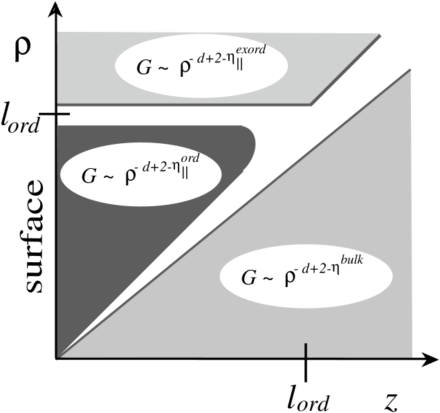
Figure 2: Regimes of universal behavior (gray areas) of the correlation function in directions parallel to the surface. The respective power laws governing the $\rho$-dependence of $G(\rho,z)$ are shown. Crossover regimes are represented as white areas.

The different regimes which the parallel correlation function $G(\rho,z,z)$ (where $\rho$ denotes the distance between two point in a plane parallel to the surface) goes through are depicted in Fig. 2. First of all, for $\rho<z$ the function $G$ asymptotically behaves as in the bulk, $G$ is governed by the bulk exponent $\eta$ (lower light gray area). In the opposite case, $\rho>z$, the result depends on whether the distance from the surface is smaller or larger than the length scale $l_{ord}$ introduced in (2.9). In the case $z>l_{ord}$ for $\rho\simeq z$ the crossover from bulk to surface behavior takes place, where $G$ is governed by the anomalous dimension of the normal transition (upper light gray area). The situation for $z<l_{ord}$ is different. Again at $\rho\simeq z$ a crossover to surface behavior takes place, to a regime $z<\rho<l_{ord}$ where the behavior is governed by exponents of the ordinary transition (dark gray area). Eventually, for $\rho\simeq l_{ord}$ the crossover to the regime with “normal” behavior takes place. In Fig. 2 the crossover regions are represented as white areas.

As we shall see in Sec. 3.3, this crossover behavior leads to the result that for instance in scattering with finite penetration depth of the radiation and $l_{ord}$ greater than this depth, the structure function is effectively governed by exponents of the ordinary transition.

2.4 Modifications at $T\neq T_{c}^{b}$

The scaling analysis presented above can be straightforwardly extended to the case $\tau>0$. In $d>2$, we may assume that the behavior near the surface for $z<<\xi$ is unchanged compared to (2.6) and (2.10). The behavior farther away from the surface depends on the ratio $l/\xi$, where $l$ stands for $l_{sp}$ or $l_{ord}$. In the case of $l>\xi$ a crossover to an exponential decay will take place for $z\simeq\xi$ and the regime of nonlinear decay $\sim z^{-\beta/\nu}$ does not occur. For $l<\xi$ a crossover to the power-law decay $\sim z^{-\beta/\nu}$ takes place for $z\simeq l$ and finally at $z\simeq\xi$ the exponential behavior sets in.

Similar results hold for the correlation functions. As long as for example the distance $\rho$ in the parallel correlation function is smaller than $\xi$, the discussion of Sec. 2.3 holds. For distances larger than $\xi$ correlations decay exponentially.

An interesting phenomenon can be observed in the case $\xi<l$. As said above, $m(z)$ then never reaches the regime with power-law decay, but crosses over from the near-surface regime directly to the exponential decay. Let us restrict the further discussion to the case of the ordinary transition. Since the region where $m(z)$ grows then only extends up to the distance $\xi$, the maximum of the OP profile has roughly the value $m_{max}\simeq{\sf h}_{1}\,\xi^{\kappa}$, where the exponent $\kappa$ was defined in (2.10). Now, the amplitude of the exponential decay should behave as $\sim m_{max}$ such that for $z\gg\xi$ we have

$$m(z)\sim{\sf h_{1}}\,\xi^{\kappa}\,\exp(-z/\xi)\>.$$ (2.12)

In other words, in the case $\xi<l_{ord}$ the exponent $\kappa$ not only governs the behavior of $m(z)$ near the surface, but also leaves its fingerprint much farther away of an universal dependence of the amplitude of the exponential decay. Nothing comparable occurs when $\xi=\infty$ (compare Sec. 2.1 above), where all profiles approach the same curve $m(z)\approx{\cal A}\,z^{-\beta/\nu}$ for $z\,\vbox{\hbox{$\buildrel\textstyle>\over{\sim}$}}l_{ord}$, with an amplitude ${\cal A}$ independent of $h_{1}$. A similar phenomenon, termed “long-time memory” of the initial condition, does also occur in critical dynamics for $T\geq T_{c}^{b}$ [24]. The analogies between surface critical phenomena and critical dynamics will be discussed in more detail in the next section.

2.5 Relation to Critical Dynamics and Heuristic Arguments

The spatial variation of the magnetization discussed so far, especially the increasing profile at the ordinary transition, strongly resembles the time dependence of the OP in relaxational processes at the critical point. If a system with nonconserved OP (model A) is quenched for example from a high-temperature initial state to the critical point, with a small initial magnetization $m^{(i)}$, the OP behaves as $m\sim m^{(i)}\,t^{\theta}$ [25], where the short-time exponent $\theta$ is governed by the difference between the scaling dimensions of initial and equilibrium magnetization divided by the dynamic (equilibrium) exponent[26]. Like the exponent $\kappa$ in (2.10), the exponent $\theta$ vanishes in MF theory, but becomes positive below $d^{*}$. For example, its value in the three-dimensional Ising model with Glauber dynamics is $\theta=0.108$ [27].

The high-temperature initial state of the relaxational process is to some extent analogous to the surface that strongly disfavors the order and that (for $h_{1}=0$) belongs to the universality class of the ordinary transition. Further expanding this analogy, heating a system from a low-temperature (ordered) initial state to the critical point would be similar to the situation at the extraordinary transition. Eventually, analogous to the special transition would be a “relaxation process” that starts from an equilibrium state at $T_{c}^{b}$.

Motivated by the analogy between surface critical phenomena and critical dynamics, an heuristic argument for the short-distance growth of the OP at the ordinary transition behavior can be brought forward. In relaxation processes, after the system has passed through a non-universal regime immediately after the quench, the growth of correlation length $\xi(t)$ is described by a power law. Analogously one may argue that in the static case in the surface-near regime there exists an effective parallel correlation length $\xi_{\parallel}(z)$ that grows as $\sim z$ when the distance $z$ grows away from the surface. As discussed in Sec. 2.3, for lateral distance $\rho\simeq z$ the parallel correlation function crosses over from “bulk” to “surface decay”, the latter being much faster than the former (compare Sec. 3.3).

For the sake of the argument, consider the semi-infinite Ising system at bulk criticality where initially $h_{1}=0$ with the tendency to order in the surface reduced compared with the bulk. If then a small $h_{1}$ is imposed on the surface, a number of spins will change their orientation to generate a small $m_{1}$. Now, the magnetization induced by in a distance $z$ from the surface is determined by several factors. First, it is proportional to $m_{1}$ and, in turn, for small $m_{1}$, it is proportional to $h_{1}$. Second, it should be proportional to the perpendicular correlation function $C(0,z)\sim z^{-d+2-\eta^{ord}_{\perp}}$ which says how much of a given surface configuration “survives” in a distance $z$. Eventually, it should be proportional to the correlated area in the distance $z$ that is influenced by a single surface spin. According to the discussion above, the latter grows as $\xi_{\parallel}^{d-1}\sim z^{d-1}$. Taking these factors together we obtain

$$m(z)\sim h_{1}\,C(0,z)\,\xi_{\parallel}^{d-1}\sim h_{1}\,z^{1-\eta^{ord}_{\perp}}\>,$$ (2.13)

in agreement with the short-distance law (2.10).

The above argument holds as long as $z$ and $m_{1}$ are small enough. If $z$ is larger than the average distance between the spins flipped, the correlated areas start to overlap and the above argument breaks down. This is where the crossover to the normal transition sets in.

From the field-theoretical point of view in both cases (surface critical phenomena and critical dynamics) the modified power laws are due to additional short-distance or short-time singularities near spatial or temporal boundaries. In both cases the singular behavior near the surface can be described by means of short-distance expansions or (in simplified form) by means of a phenomenological scaling analysis as presented above. It is interesting to point out, however, that in the presence of both spatial and temporal boundaries no additional singularities (other than the ones discussed above) occur [28], and, as a consequence, the short-time behavior in critical dynamics near surfaces is governed by exponents that can be expressed in terms of known surface and dynamic exponents[28].

3 Mean-field (Zero-Loop) Approximation

In this section we define the model and describe the results of the MF theory for general $c$ and $h_{1}$. They are the building blocks for the (one-loop) perturbative calculation of Sec. 4. Especially the zero-loop propagator for general $c$ and $h_{1}$ is not contained in explicit form in the literature so far. Further in Sec. 3.3 we discuss the behavior of the real-space correlation function and the respective structure function that is measured for instance in X-ray scattering experiments. The one-loop calculation for this quantity for general $c$ and $h_{1}$ is not attempted in the present work. So the MF results presented here are not only the best presently available in the framework of continuum field theory, but also provide, as we think, a qualitative description of the results to be expected from scattering experiments.

3.1 Model

We consider the semi-infinite scalar $\phi^{4}$ with the Hamiltonian[2]

$${\cal H}=\int_{V}\left[\frac{1}{2}(\nabla\phi)^{2}+\frac{1}{2}\tau\,\phi^{2}+\frac{1}{4!}u\,\phi^{4}\right]+\int_{\partial V}\left[\frac{1}{2}c\,\phi^{2}+h_{1}\,\phi\right]\>,$$ (3.1)

where $V$ and $\partial V$ stand for the volume of the semi-infinite system and its (planar) surface, respectively.

The well-known solution to the OP profile, minimizing the above Hamiltonian, takes the form[29, 14, 12]

$$m^{(0)}(z)=\alpha^{-1}(z+z^{+})^{-1}\>,$$ (3.2)

where the length scale $z^{+}$ is given by

$$z^{+}=\frac{c+\sqrt{c^{2}+4h_{1}\alpha}}{2\alpha h_{1}}$$ (3.3)

and

$$\alpha=\sqrt{\frac{u}{12}}\>.$$ (3.4)

The solution (3.2) satisfies the general (mixed) boundary condition

$$\frac{\partial\,m}{\partial z}=c\,m-h_{1}\>.$$ (3.5)

The MF solution to the OP profile has a fairly simple form. Consistent with the discussion in Secs. 1 and 2, it is a monotonic function of $z$. Further, although $c$ and $h_{1}$ in principle give rise to two independent length scales, in the OP profile they show up in a single length scale $z^{+}$ only. As a consequence, the shape of the profile does not change qualitatively when one moves from one fixed point to the other.

3.2 Free Propagator

The two-point correlation function for general $c$ and $h_{1}$ that will be described next solves the equation

$$\left[-\nabla^{2}+\frac{1}{2}\,u\,m^{2}(z)\right]G({\bf x},{\bf x}^{\prime})=\delta({\bf x}-{\bf x}^{\prime})\>,$$ (3.6)

subject to the boundary condition (at $z=0$)

$$\left[\frac{\partial}{\partial z}-c\right]G({\bf x},{\bf x}^{\prime})|_{z=0}=0\>,$$ (3.7)

where $m^{(0)}(z)$ is the profile of (3.2). To calculate $G$ we Fourier transform with respect to the parallel, translationally invariant spatial directions. The result that can be obtained by standard methods reads

$$\hat{G}({\bf p};z,z^{\prime})=\theta(z-z^{\prime})W(p,z)U(p,z^{\prime})+\theta(z^{\prime}-z)W(p,z^{\prime})U(p,z)\>,$$ (3.8)

where $p=|{\bf p}|$, $\theta(z)$ is the Heaviside step function, and the function $W$ and $U$ are given by

$$W(p,z)=\left[p^{2}+\frac{3p}{z+z^{+}}+\frac{3}{(z+z^{+})^{2}}\right]e^{-pz}$$ (3.9)

and

$$U(p,z) = \frac{1}{2p^{5}}\left\{B(p)\left[p^{2}+\frac{3p}{z+z^{+}}+\frac{3}{(z+z^{+})^{2}}\right]e^{-pz}\right.$$ (3.10)

$$\hskip 71.13188pt\left.+\left[p^{2}-\frac{3p}{z+z^{+}}+\frac{3}{(z+z^{+})^{2}}\right]e^{pz}\right\}$$

with

$$B(p)=\frac{k^{3}-k^{2}(q+1)+3kq-3q}{k^{3}+k^{2}(q+1)+3kq+3q}\>.$$ (3.11)

Further, we introduced a dimensionless wave vector

$$k=p\,z^{+}$$ (3.12)

and, for the sake of brevity, we defined

$$q=2+c\,z^{+}\>.$$ (3.13)

The length scale $z^{+}$ was already introduced in (3.3).

In contrast to the OP profile, the MF correlation function now depends on two length scales. In addition to the dependence on $z^{+}$, it contains via the quantity $q$ defined in (3.13) an explicit $c$-dependence. The latter defines the second length scale $l_{c}\equiv c^{-1}$.

For the correlation function $\hat{G}({\bf p};z,z)$ and the for the propagator at ${\bf p}=0$, one obtains from (3.8)

$$\hat{G}({\bf p};z,z) = \frac{1}{2p^{5}}\left\{B(p)\left[p^{2}+\frac{3p}{z+z^{+}}+\frac{3}{(z+z^{+})^{2}}\right]^{2}e^{-2pz}\right.$$ (3.14)

$$\left.\hskip 71.13188pt+p^{4}-\frac{3p^{2}}{(z+z^{+})^{2}}+\frac{9}{(z+z^{+})^{4}}\right\}$$

and

$$\hat{G}(0;z,z^{\prime}) = \left.\frac{1}{5}\;\right\{(z+z^{+})^{-2}\times$$ (3.15)

$$\left.\left[\frac{5-q}{q}\,(z^{+})^{5}\,(z^{\prime}+z^{+})^{-2}+(z^{\prime}+z^{+})^{3}\right]\theta(z-z^{\prime})+(z\leftrightarrow z^{\prime})\right\}\>,$$

respectively. The results (3.14) and (3.15) are needed in Sec. 4 to calculate the one-loop contributions to the OP profile.

3.3 Structure Function for Critical Diffuse Scattering

A quantity directly relevant for experiments is the structure function

$$\tilde{S}(p,\kappa)=A\,\int_{0}^{\infty}\int_{0}^{\infty}\hat{G}({\bf p},\,z,\,z^{\prime})\,e^{i(\kappa z-\kappa^{*}z^{\prime})}\,dz\,dz^{\prime}\>,$$ (3.16)

where $A$ is a constant – for a cubic lattice it is just the illuminated area divided by a power of the lattice constant – and $\kappa=\kappa_{r}+i\,\kappa_{i}$ is a complex wavenumber taking into account that the radiation penetrates the material roughly up to the depth $\kappa_{i}^{-1}$ [4].

Analytic results for $\tilde{S}$ on the basis of (3.8) can be obtained at or near the fixed points only, where the correlation function turns out to be much simpler than the general expression (3.8). Here we present the analytic results for the ordinary and the extraordinary (or normal) transition and evaluate the transformation (3.16) numerically in the crossover regime, i.e. for large $c$ and and arbitrary $h_{1}/c$. The latter is the generic situation met in systems where the spin-spin interaction near the surface is not enhanced and where the surface spins are coupled to an external (non-critical) medium that favors one of the spin directions. The results presented below were obtained by setting $q=\infty$ in (3.8) (thus ignoring corrections of order $c^{-1}$). Then the function $B(p)$ becomes

$$\lim_{c\to\infty}\,B(p)=-\frac{k^{2}-3k+3}{k^{2}+3k+3}\>,$$ (3.17)

and the length scale $z^{+}$ from (3.3) is to be identified with the length scale $l_{ord}$ introduced in Sec. 2.1. Again in leading order in $c^{-1}$ one obtains

$$l_{ord}=z^{+}=\frac{c}{\alpha h_{1}}\>,$$ (3.18)

consistent with the scaling analysis in Sec. 2.1 and with the fact that $y=1$ in MF theory.

By general arguments (scaling analysis and short-distance expansion) it was shown by Dietrich and Wagner[4] that in the limit $p\to 0$ the structure function takes the form

$$\tilde{S}(p,\kappa)=s_{0}(\kappa)-s_{1}(\kappa)\,p^{\eta_{\parallel}-1}\>.$$ (3.19)

Explicit results were obtained in Ref. [4] at the ordinary transition up to one-loop order.

Starting from (3.8) our result for the ordinary transition ($\tau=h_{1}=0,\,c=\infty$) is

$$A^{-1}\,\tilde{S}(p,\kappa)=\frac{1}{2\,\kappa_{i}\,|\kappa|^{2}}-\frac{p}{|\kappa|^{4}}\>,$$ (3.20)

in consistency with Ref. [4]. For the normal transition ($\tau=0,\,c=h_{1}=\infty$) we obtain

$$A^{-1}\,\tilde{S}(p,\kappa)=\frac{1}{20\,\kappa_{i}^{3}}\,\Re\left[{}_{2}F_{1}(1,3,5,i\,\kappa_{i}^{-1}\kappa/2)\right]-\frac{12}{75}\,\frac{p^{5}}{|\kappa|^{8}}\>,$$ (3.21)

where ${}_{2}F_{1}$ is the hypergeometric function [30] and $\Re$ denotes the real part of the term in square brackets. The MF values of $\eta_{\parallel}$ are $2$ for the ordinary transition and $6$ for the normal transition, respectively, and so the results (3.20) and (3.21) are consistent with (3.19).

Figure 3: The MF structure function for critical diffuse scattering defined in (3.16) in the crosover regime between ordinary and normal transition for different values of $l_{ord}\,\kappa_{i}$ (solid lines). The upper dashed line shows the asymptotic ($p\to 0$) result at the ordinary transition given in (3.20). The lower dashed line is the analogous curve at the normal transition of (3.21).

As the next step the transformation (3.16) is carried out numerically in the crossover regime between ordinary and normal transition. The result can certainly not be compared with experiments on a quantitative level – the real exponents differ significantly from their MF values – , but it should give the qualitative picture that one has to expect from a (Gedanken)experiment carried out in a system at bulk criticality with adjustable scaling field $h_{1}/c$ and otherwise fixed parameters.

The results for $\tilde{S}$ for the particular choice $\kappa_{r}=\kappa_{i}$ are depicted in Fig. 3 (solid lines). For $\hat{l}\equiv l_{ord}\cdot\kappa_{i}\gg 1$, the $p\to 0$ limit of $\tilde{S}$ has effectively the cusp shape typical for ordinary transition. (In contrast to the situation in the bulk, $\tilde{S}$ never diverges[4], because in the surface-near regime (which at $T_{c}^{b}$ extends to infinity) the long-distance decay of correlations is much faster than in the bulk.) For smaller values of $\hat{l}$, it becomes visible that for small momenta $p\,l_{ord}\ll 1$ the behavior is actually described by the anomalous dimension of the normal transition, leading to a curve without cusp departing with slope zero from $p=0$. For comparison we have also plotted the asymptotic results for $p\to 0$ and $l_{ord}=0$ and $\infty$ (dashed lines).

4 One-Loop Calculation of the Order-Parameter Profile

In this section we calculate the OP profile in the framework of the $\epsilon$-expansion (where $\epsilon\equiv 4-d$) near both the ordinary and special fixed point, the latter mainly with regard to the crossover between special and ordinary transition. For the sake of simplicity, all calculations are restricted to $\tau=0$. In the following we first give the results for the one-loop contribution to $m(z)$. They are regularized dimensionally in $d=4-\epsilon$ dimensions and renormalized by minimal subtraction. After focussing attention on the short-distance behavior of the OP, we calculate the full scaling functions up to first order in $\epsilon$ near both the ordinary and the special transition. Finally we present results on the crossover between special and ordinary near-surface behavior.

In order to remove the UV divergences appearing in the one-loop term, the parameters $u$, $c$, and $h_{1}$ of Sec. 3 have to be considered as bare parameters labelled with an index ‘0’ below. In the standard procedure, dimensional regularization combined with minimal subtraction[2], the bare parameters are replaced by renormalized ones to obtain a UV finite expression for $m(z)$. The field $\phi$ which in general also has to be renormalized is unchanged up to order $\epsilon$, such that we do not have to worry about wavefunction renormalization in the present work. Further, in dimensional regularization the fixed point value $c^{*}$ of the surface enhancement remains at zero such that $\tilde{c}=c$.

4.1 Perturbation Expansion

Expanding in terms of the coupling constant $u_{0}$, $m(z)$ can be written in the form

$$m(z)=m^{(0)}(z)+m^{(1)}(z)+O(u_{0}^{2})\>,$$ (4.1)

where the MF solution $m^{(0)}$ was given in (3.2) and the first-order term $m^{(1)}$ is

$$m^{(1)}(z)=-\frac{u_{0}}{2}\int_{0}^{\infty}dz^{\prime}\,\hat{G}({\bf 0},z,z^{\prime})\int_{\bf p}\hat{G}({\bf p},z^{\prime},z^{\prime})\,m^{(0)}(z^{\prime})$$ (4.2)

with $\int_{\bf p}\equiv(2\pi)^{-d+1}\int\,d^{d-1}p$. Using the results (3.2), (3.14), and (3.15), the $z^{\prime}$ integration in (4.2) can be carried out. This yields the result

$$m^{(1)}=-\frac{u_{0}s_{d}\sqrt{\pi}}{z^{+}\,\Gamma\left((3-\epsilon)/2\right)}\alpha^{-1}X\,\int_{0}^{\infty}dk\,k^{-\epsilon}\,I$$ (4.3)

where $s_{d}=(2\sqrt{\pi})^{-d}$, and the integrand $I$ is given by

$$I=-B\,F\,e^{-2k\,z/z^{+}}+\frac{3}{2}\,X\left[\left(B+1\right)\left(1+\frac{1}{q}\right)-X\right]k^{-3}+\frac{1}{2q}XB$$ (4.4)

$$\hskip 34.1433pt+\frac{1}{4q}\left[B\,X(q+9)+3X(q-1)-3q\right]k^{-1}$$

$$\hskip 34.1433pt+\left(\frac{X^{2}}{2q}+\frac{1}{6X}-\frac{X^{2}}{6}+B\,X\left(\frac{5}{4}+\frac{3}{q}\right)k^{-2}\right)k\>,$$

where $q$ and $k$ were defined in (3.13) and (3.12), respectively. Further, we introduced

$$X=\frac{z^{+}}{z+z^{+}}$$ (4.5)

with $z^{+}$ defined in (3.3) and

$$F=\frac{1}{4}k^{-1}+\frac{5}{4}Xk^{-2}+\frac{3}{2}X^{2}k^{-3}\>.$$ (4.6)

4.2 Renormalization of UV Divergences and Short-Distance Singularities

The perturbative result (4.3) contains UV singularities which show up as poles $\propto\epsilon^{-1}$ in dimensional regularization. These poles are removed by minimal subtraction[2, 31], by expressing the bare parameters occurring in $m^{(0)}$ in terms of renormalized ones. The relation between bare and renormalized coupling is given by

$$u_{0}\,s_{d}=\mu^{\epsilon}\,u\left[1+\frac{3u}{\epsilon}+{\cal O}(u^{2})\right]\>,$$ (4.7)

where $\mu$ is an arbitrary momentum set to $1$ afterwards. Further, near the special transition, for finite $c$ and $h_{1}$, the renormalizations are

$$c_{0}=\mu c\left[1+\frac{u}{\epsilon}+{\cal O}(u^{2})\right]$$ (4.8)

and

$$h_{1,0}=\mu^{d/2}h_{1}\left[1+\frac{u}{2\epsilon}+{\cal O}(u^{2})\right]\>.$$ (4.9)

At the ordinary transition, for $c\to\infty$ with finite ${\sf h}_{1}=h_{1}/c$, we have

$${\sf h}_{1,0}=\mu^{d/2}{\sf h}_{1}\left[1+\frac{u}{2\epsilon}+{\cal O}(u^{2})\right]\>.$$ (4.10)

Up to first order in $\epsilon$ the renormalization of $h_{1}$ and ${\sf h}_{1}$ are the same, but taking into account higher orders in $\epsilon$ they are different[2]. In both cases the poles are removed and one is left with an expression for $m(z)$ that is regular in $\epsilon$ and $u$.

In our first-order perturbative calculation, modifications of the short-distance behavior of the OP profile show up in the form of logarithmic (short-distance) singularities of $m^{(1)}$. The source of these logarithms in our result (4.3) is the first term on the right-hand side of (4.4). Focussing the attention for the moment on the short-distance behavior only, (4.3) can be written as

$$m(z)=\frac{u\,s_{d}\,X}{2\,z^{+}\alpha}J_{sing}+\mbox{terms regular for $z\to 0$}\>,$$ (4.11)

where $J_{sing}$ is given by

$$J_{sing}=\int_{1}^{\infty}dk\,B\,k^{-1-\epsilon}\,e^{-2k\,z/z^{+}}\>.$$ (4.12)

For a closer inspection of the $z\to 0$ limit of this integral, it is useful to rewrite the function $B$ (defined in (3.11)) in the equivalent forms

$$B=1-2b_{sp}=-1+2kb_{ord}$$ (4.13)

with

$$b_{sp}=\frac{(q+1)k^{2}+3q}{k^{3}+(q+1)k^{2}+3qk+3q}$$ (4.14)

and

$$b_{ord}=\frac{k^{2}+3q}{k^{3}+(q+1)k^{2}+3qk+3q}\>.$$ (4.15)

While $b_{sp}$ yields regular terms for general $c$ and $h_{1}$, in the second form $b_{ord}$ leads to finite contributions after taking the limit $c\to\infty$:

$$\lim_{c\to\infty}b_{ord}\equiv b_{\infty}=\frac{3}{k^{2}+3k+3}\>.$$ (4.16)

With (4.14) and (4.15), $J_{sing}$ can be written as

$$J_{sing}\!=\!\!\int_{1}^{cz^{+}}\!\!dk(2kb_{ord}-1)k^{-1-\epsilon}e^{-2kz/z^{+}}\!\!+\!\!\int_{cz^{+}}^{\infty}\!\!dk(1-2b_{sp})k^{-1-\epsilon}e^{-2kz/z^{+}}\!\!,$$ (4.17)

where we assumed that $cz^{+}>1$. Alternatively, after straightforward manipulations, it can be expressed in the form

$$J_{sing}\!=\!\int_{1}^{\infty}dkk^{-1-\epsilon}\!\left(2e^{-2kz/l_{c}}-e^{-2kz/z^{+}}\right)\!+\!\mbox{terms regular for $z\to 0$ }\!,$$ (4.18)

where $l_{c}\equiv c^{-1}$ is the length scale induced by the surface enhancement.

To discuss the crossover between special and ordinary near-surface behavior, we assume $c$ to be large and $l_{c}\ll z^{+}\simeq l_{ord}$. From (4.18) it becomes then apparent that for $z\ll l_{c}$

$$J_{sing}=\log z+\mbox{terms regular for $z\to 0$ }\>.$$ (4.19)

For $l_{c}\ll z\ll z^{+}$, on the other hand, the first term in the integral in (4.18) is negligible, and we obtain

$$J_{sing}=-\log z+\mbox{terms regular for $z\to 0$ }\>,$$ (4.20)

which also holds for $c\to\infty$ and $z\ll z^{+}$, i.e., it describes the short-distance singularity at the ordinary transition.

If eventually the coupling constant $u$ is set to its fixed-point value $u^{*}=\epsilon/3$ and the logarithms are exponentiated, we find

$$m(z)\sim\left\{\begin{array}[]{ll}1-\frac{\epsilon}{6}\log z+O(\epsilon^{2})\sim z^{-\epsilon/6}&\mbox{for $z\ll l_{c}$}\\[11.38109pt] 1+\frac{\epsilon}{6}\log z+O(\epsilon^{2})\sim z^{\epsilon/6}&\mbox{for $l_{c}\ll z\ll l_{ord}$}\end{array}\right.\>.$$ (4.21)

The exponents $\epsilon/6$ and $-\epsilon/6$ are to be identified with the first-order values for $1-\eta_{\perp}^{ord}$ and $(\beta_{1}^{sp}-\beta)/\nu$, respectively [2]. In general, for finite $cz^{+}$ both terms in (4.17) give non-negligible contributions, each on the respective length scale, i.e. the first term only for $z\ll l_{c}$, the second one for $z\ll l_{ord}$. This is consistent with our qualitative discussion in Sec. 2.2.

4.3 Scaling Function at the Ordinary Transition.

The procedures for obtaining the scaling function at the ordinary and the special transition are similar. We describe the first case in more detail. For $c\to\infty$, after the subtraction of pole terms with (4.7) and (4.10), the perturbative results (4.1) and (4.3) take the form

$$m(z)=m^{0}(z;u,{\sf h}_{1})-\frac{2us_{d}X}{z^{+}\alpha}\left[\int_{0}^{\infty}dk\,C^{ord}+\frac{1}{4}\left(2X-3\right)\log z^{+}\right]\>,$$ (4.22)

where

$$C^{ord} = {F}(1-b_{\infty})e^{-2kz/{z^{+}}}+\frac{3}{2}X(b_{\infty}-X)k^{-3}+\frac{5}{4}X(b_{\infty}-1)k^{-2}$$ (4.23)

$$+ \frac{1}{4}(2X-3)\frac{1}{k(k+1)}+\frac{1}{4}b_{\infty}Xk^{-1}$$

is obtained from $I$ (defined in (4.4)) by setting $q=c=\infty$. In dimensional regularization terms of order $O(k^{0})$ and $O(k^{1})$ present in (4.4) give vanishing contributions to the integral and are omitted here. As the next step we utilize the scaling form (2.8), derived on a more rigorous level with the help of the renormalization group [2]. The scaling function is given by

$${\cal M}_{ord}(\zeta)=m(z=1,\bar{u}=u^{*},\bar{\sf h}_{1}(\zeta)={\sf h}_{1}z^{\Delta_{1}^{ord}/\nu})\>,$$ (4.24)

where the scaled distance $\zeta$ is

$${\zeta}=\frac{z}{l_{ord}}\qquad\mbox{with}\qquad l_{ord}=\left(\alpha^{*}\,{\sf h}_{1}\right)^{-\nu/\Delta_{1}^{ord}}\>,$$ (4.25)

and $\alpha^{*}$ is defined by (3.4) with $u=u^{*}$.

The result (4.22) gives the scaling function up to terms $O(\epsilon^{2})$ according to the equation

$${\cal M}_{ord}(\zeta)=m^{(0)}(1,u^{*},{\sf h}_{1}z^{\Delta_{1}^{ord}/\nu})+m^{(1)}(1,u^{*},{\sf h}_{1}z^{\Delta_{1}^{ord}/\nu})+O(\epsilon^{2})\>$$ (4.26)

The MF result (3.2), after substituting $z\to 1$ and

$$z^{+}\to(\alpha^{*}{\sf h}_{1})^{-1}z^{-\Delta_{1}^{ord}/\nu}=\zeta^{-1}\left(1+\frac{\epsilon}{3}\log\zeta\right)+O(\epsilon^{2})$$ (4.27)

reads

$$m^{(0)}(z=1,\bar{u}=u^{*},\bar{\sf h}_{1}={\sf h}_{1}z^{\Delta_{1}^{ord}/\nu}) =$$ (4.28)

$$(\alpha^{*})^{-1}\frac{\zeta}{1+\zeta}\left(1-\frac{\epsilon}{3}\frac{1}{1+\zeta}\log\,\zeta\right)+O(\epsilon^{2})\>.$$

Together with the one-loop contribution (4.22), we obtain for the scaling function

$${\cal M}_{ord}(\zeta)=(\alpha^{*})^{-1}\frac{\zeta}{1+\zeta}\left[1-\epsilon\,\left(\frac{1}{2}\log\zeta+\frac{2}{3}\int_{0}^{\infty}dk\,C^{ord}\right)\right]+{\cal O}(\epsilon^{2})\>.$$ (4.29)

One can easily check that for $\zeta\to 0$ the integral $\int_{0}^{\infty}dk\,C^{ord}$ behaves as $\sim-\frac{1}{4}\log\zeta+$ regular terms, and, as a consequence, the short-distance limit of the scaling function is given by

$${\cal M}_{ord}(\zeta)\sim\zeta\left[1-\frac{\epsilon}{3}\log\zeta\right]+{\cal O}(\epsilon^{2})\>.$$ (4.30)

Taking into account that $\beta/\nu=1-\epsilon/2+{\cal O}(\epsilon^{2})$ such that $z^{-\beta/\nu}=z^{-1}(1+\epsilon/2\,\log z+{\cal O}(\epsilon^{2})$), this is consistent with (4.21) and, hence, with the result (2.10) of our scaling analysis. Furthermore, it is straightforward to show that ${\cal M}_{ord}$ approaches a constant for $\zeta\to\infty$.

Figure 4: Scaling function $\widehat{\cal M}_{ord}$ for the crossover between ordinary and normal transtion defined in (4.32) for $\epsilon=1$ (solid), 0.4 (dashed), and 0.1 (dotted line).

In order to exponentiate the scaling function in the short-distance regime, we effectively replace the logarithm of (4.30) by the power law $\zeta^{1-\epsilon/3}$, the exponent $1-\epsilon/3$ being the one-loop value of $\Delta_{1}^{ord}/\nu$. This is achieved by adding

$${\cal G}_{ord}=e^{-\zeta^{2}}\left[\zeta^{1-\epsilon/3}-\zeta\left(1-\frac{\epsilon}{3}\log\zeta\right)\right],$$ (4.31)

to (4.29), a function of ${\cal O}(\epsilon^{2})$.

The result for the OP as a function of $\zeta$, i.e. the function

$$\widehat{\cal M}_{ord}=\zeta^{-1+\epsilon/2}({\cal G}_{ord}+\alpha^{*}{\cal M}_{ord})\>,$$ (4.32)

is depicted in double-logarithmic representation for three different values of $\epsilon$ in Fig. 4. The integral in (4.29) had to be calculated numerically. All profiles show the characteristic crossover between short-distance growth and long-distance decay. However, extrapolating $\epsilon$ to one obviously leaves us with a profile with somewhat unexpected features. It has a point of inflection were one actually expects a smoother scaling function. On the other hand, for the smaller values of $\epsilon$ this problem does not exist. So we think that extrapolating $\epsilon$ to 1 in (4.29) probably just at the limit, where the first-order result ceases to provide a good approximation.

4.4 Scaling Function at the Special Transition and Crossover to the Ordinary Transition

For arbitrary $c$ we proceed as before, now with the renormalization of the surface parameters given by (4.8) and (4.9). The perturbative result for the profile (4.1) is [13]

$$m(z)=m^{(0)}(z;u,c,h_{1})\!-\!\frac{2us_{d}X}{z^{+}\alpha}\left[\int_{0}^{\infty}dk\,C(k)\!+\!\frac{1}{2}\left(\frac{X}{q}-\frac{3}{2}\right)\log z^{+}\right]\!,$$ (4.33)

where we extracted the regular contribution

$$C = (2b_{sp}-1)\,F\,e^{-2kz/{z^{+}}}+\frac{3}{2}X\left[2(1-b_{sp})\left(1+\frac{1}{q}\right)-X\right]k^{-3}$$ (4.34)

$$- \frac{(q+9)X}{2q}b_{sp}k^{-1}+\left(\frac{5}{4}+\frac{3}{q}\right)(1-2b_{sp})X\,k^{-2}$$

$$+ \frac{1}{2}\left(\frac{X}{q}-\frac{3}{2}\right)\frac{1}{k(k+1)}-\left(b_{sp}-\frac{q+1}{k}\right)\frac{X}{q}$$

from $I$ of (4.4).

At the special transition, alternatively to (2.2), the order parameter can be expressed in the scaling form

$$m(z;u,\bar{c},\bar{h}_{1})=z^{-\beta/\nu}{\cal M}(\zeta,\gamma)$$ (4.35)

with

$${\cal M}(\zeta,\gamma) = m(z=1;\bar{u}=u^{*},\bar{c}(\zeta,\gamma)=cz^{\phi/\nu},\bar{h}_{1}(\zeta)=h_{1}z^{\Delta_{1}^{sp}/\nu})$$ (4.36)

$$=m^{(0)}(1;u^{*},cz^{\Phi/\nu},h_{1}z^{\Delta_{1}^{sp}/\nu})+m^{(1)}(1;u^{*},cz^{\Phi/\nu},h_{1}z^{\Delta_{1}^{sp}/\nu})+O(\epsilon^{2})$$

where

$$\zeta=\frac{z}{l_{sp}}\>,\quad\gamma=ch_{1}^{-\Phi/\Delta_{1}^{sp}}\>,\quad\mbox{and}\quad l_{sp}=\left(\alpha^{*}\,h_{1}\right)^{-\nu/\Delta_{1}^{sp}}\>.$$ (4.37)

Expressing all the parameters in terms of scaling variables $\zeta$ and $\gamma$ and keeping terms to first order in $\epsilon$ in the MF contribution and to zeroth order in $\epsilon$ in the one-loop term, we obtain the result

$${\cal M}(\zeta,\gamma) = (\alpha^{*})^{-1}\frac{\zeta}{\zeta+\zeta_{0}}\left\{1-\frac{\epsilon}{3}\left[\frac{1}{q}\frac{\zeta_{0}}{\zeta+\zeta_{0}}\log\zeta_{0}\right.\right.$$ (4.38)

$$\hskip 56.9055pt+\left.\left.\frac{3}{2}\log\left(\frac{\zeta}{\zeta_{0}}\right)+2\int_{0}^{\infty}dk\,C(k)\right]\right\}+O(\epsilon^{2})\>,$$

where

$$\zeta_{0}=\frac{1}{2}\left(\gamma+\sqrt{\gamma^{2}+4}\right)$$ (4.39)

and the integrand $C$ is given by (4.34) with $z=1$, $z^{+}=\zeta_{0}/\zeta$, and $q=2+\zeta_{0}\gamma$.

It is straightforward to verify that the short-distance behavior of the OP described by (4.38) for a system with $\gamma\gg 1$ is consistent with the discussion in Sec. 4.2, especially with (4.21). The short-distance logarithm in (4.38) is caused by the first term on the right-hand side of (4.34). One obtains

$${\cal M}(\zeta,\gamma)\sim\frac{\zeta}{\zeta_{0}}\left[1-\frac{2}{3}\epsilon\log\left(\frac{\zeta}{\zeta_{0}}\right)\right]+{\cal O}(\epsilon^{2})$$ (4.40)

for $\zeta/\zeta_{0}\ll q^{-1}$ (equivalent to $z\ll l_{c}$), which, together with the prefactor $\sim\zeta^{-\beta/\nu}$ (see (4.35)), is consistent with the upper line in (4.21) and with Refs. [12, 13]. And one finds

$${\cal M}(\zeta,\gamma)\sim\frac{\zeta}{\zeta_{0}}\left[1-\frac{1}{3}\epsilon\log\left(\frac{\zeta}{\zeta_{0}}\right)\right]+{\cal O}(\epsilon^{2})$$ (4.41)

for $q^{-1}\ll\zeta/\zeta_{0}\ll 1$ (equivalent to $l_{c}\ll z\ll l_{ord}$), in agreement with the second case in (4.21).

The crossover between the two asymptotic cases occurs at the length scale $l_{sp}$, which is the intermediate scale between $l_{c}$ and $l_{ord}$. The ratio between all the scales is set by the single parameter $\gamma$ of (4.37), and from the definitions of the length scales (2.3), (2.9) and $\gamma$ we find

$$\frac{l^{ord}}{l^{sp}}=\gamma^{y\nu/{\Delta_{1}^{ord}}}\qquad\mbox{and}\qquad\frac{l^{sp}}{l_{c}}=\gamma^{\nu/\phi}\>.$$ (4.42)

At the special transition, $\gamma=0$, the scaling function is given by ${\cal M}_{sp}={\cal M}(\zeta,\gamma=0)$, with ${\cal M}$ given by (4.38). Like at the ordinary transition we exponentiate the short-distance logarithm by adding the ${\cal O}(\epsilon^{2})$ function

$${\cal G}_{sp}=e^{-\zeta^{2}}\left[\zeta^{1-2\epsilon/3}-\zeta\left(1-\frac{2}{3}\epsilon\log\zeta\right)\right]\>,$$ (4.43)

where the exponent $1-2\epsilon/3$ is the first-order value for $\beta_{1}^{sp}/\nu$. The OP scaling function

$$\widehat{\cal M}_{sp}=\zeta^{-1+\epsilon/2}\left({\cal G}_{sp}+\alpha^{*}{\cal M}_{sp}\right)\$$ (4.44)

is depicted in Fig. 5 for three values of $\epsilon$. All profiles correctly show the asymptotic power laws for short and long distances, respectively. Like the result for the ordinary transition, however, the curve for $\epsilon=1$ exhibits unexpected features. This becomes clearer visible, when one plots the scaling function ${\cal M}_{sp}$ directly, without exponentiation, i.e. the result (4.38) with $\gamma=1$. The result is shown in Fig. 6 (upper curve). For $z\to 0$, ${\cal M}_{sp}$ behaves as $\sim\log\zeta$, and for $\zeta\to\infty$ it approaches a constant. As seen from Fig. 6, it varies between the two asymptotic limits in a non-monotonic fashion, where one actually expects a monotonic variation. The reason for this qualitative defect was already discussed at the end of Sec. 4.3.

Figure 5: Scaling function $\widehat{\cal M}_{sp}$ for the crossover between special and normal transition defined in (4.44) for $\epsilon=1$ (solid), 0.4 (dashed), and 0.1 (dotted line).

What happens if $\gamma$ takes intermediate values, between the fixed points $\gamma=0$ (special) and $\gamma=\infty$ (ordinary)? The results for ${\cal M}(\zeta,\gamma)$ of (4.38) for $\gamma=0$, 1, 5, 10, and 15 and $\epsilon=1$ are displayed in Fig. 6 (from top to bottom). For increasing $\gamma$ the profiles first become monotonic functions and then, for $\gamma\,\vbox{\hbox{$\buildrel\textstyle>\over{\sim}$}}1$, a minimum occurs. This is the signature of the crossover between special and ordinary transition. Consistent with the qualitative discussion in Sec. 2.2, drops first and then increases again to approach a constant. However, for larger values $\gamma\,\vbox{\hbox{$\buildrel\textstyle>\over{\sim}$}}15$ the scaling function ${\cal M}$ becomes negative, signaling that the one-loop result calculated at the special transition becomes meaningless at intermediate values of $\zeta$. This time the problem is not cured by going to smaller $\epsilon$; for large $\gamma$ the scaling function ${\cal M}$ becomes still negative.

Figure 6: The (unexponeniated) scaling function ${\cal M}$ of (4.38) for different values of $\gamma$ and $\epsilon=1$.

Figure 7: Scaling function $\widehat{\cal M}$ for the order parameter in the crossover regime between special and normal transtion defined in (4.45) for different values of $\gamma$ and $\epsilon=1$.

Eventually in Fig. 7 we have plotted the function

$$\widehat{\cal M}=\zeta^{-1+\epsilon/2}\left({\cal G}_{sp}+\alpha^{*}{\cal M}\right)\>,$$ (4.45)

where ${\cal G}_{sp}$ is defined in (4.43), for the same values of $\gamma$ as in Fig. 6. All curves have the expected power-law form for small and large arguments. For intermediate values up to $\gamma\simeq 10$, the behavior is reminiscent to the qualitative picture described in Sec. 2.2 and depicted in Fig. 1. For larger $\gamma\,\vbox{\hbox{$\buildrel\textstyle>\over{\sim}$}}15$ the OP becomes negative for intermediate $z/l_{sp}$.

5 Summary and Concluding Remarks

We studied a semi-infinite Ising-like system by means of continuum field theory. Particular attention was paid to situations where the surface enhancement $c$ and the magnetic field $h_{1}$ are off their fixed-point values, in which case they may give rise to macroscopic length scales (in addition to $\xi$) and anomalous behavior of thermodynamic quantities near the surface. We carried out a phenomenological scaling analysis and discussed the near-surface phenomena from various points of view, especially analogies with in critical dynamics were pointed out. Furthermore, we presented mean-field results for the structure function in the crossover regime between ordinary and normal transition, and we carried out a first-order calculation for the order-parameter in the framework of renormalization-group perturbation theory ($\epsilon$-expansion).

Let us conclude by highlighting the main results of this work. The structure functions displayed in Fig. 3 may, on a qualitative level, directly be compared to the outcome of scattering experiments, like the one carried out by Mailänder et al. [5]. Our results show that in the case when the length $l_{ord}$ is larger than the penetration depth of the radiation $\kappa_{i}^{-1}$, the structure function is effectively governed by the exponent of the ordinary transition and shows the cusp for $p\to 0$ predicted in Ref. [4]. Only when the product $l_{ord}\cdot\kappa_{i}$ is smaller, the signature of the normal transition, a “flat” structure function, can be seen.

Further, the order-parameter profiles for the crossover between ordinary and normal transition displayed in Fig. 4 supplement earlier studies which focussed on various other aspects of the near-surface behavior[18, 19, 20]. Although extrapolating $\epsilon$ to one in our results appeared to be rather courageous, we believe that with these profiles a quantitative comparison with experimental data should be feasible. The Monte Carlo data available at present[19], although obtained from relatively large systems with up to $256^{2}\times 512$ spins, are still distorted by large finite-size effects and can not yet compete with the results presented in this work, where really the situation in the semi-infinite system is described.

Eventually, the crossover between special and ordinary transition was studied on the basis of the first-order perturbative approximation. In principle the results for general $c$ and $h_{1}$ presented in Sec. 4.4 should cover this crossover as the limit $c\to\infty$. The qualitative scenario was described in Sec. 2.2. In our first-order calculation we found that, while the asymptotics for small and large $z$ remain correct (compare also (4.21), the one-loop contribution becomes larger than the zero-loop term for intermediate $z$, and the order-parameter profile becomes even negative for large $c$ (see Figs. 6 and 7). This means, in other words, that the first-order approximation breaks down in this limit, at least for intermediate distances, where the crossover from $z^{(\beta_{1}^{sp}-\beta)/\nu}$ (characteristic for the special transition) to $z^{(\Delta_{1}^{ord}-\beta)/\nu}$ (characteristic for the ordinary transition) should occur. The reason for the failure of the first-order approximation is connected to different UV divergences at the ordinary and special transition, which, in the framework of the $\epsilon$-expansion, are intimately related to the short-distance singularities. This problem could probably be solved by introducing a cutoff, which, from the physical point of view, would certainly be meaningful, and consider the ordinary transition as the case where the surface enhancement $c$ is of the order of the cutoff (as opposed to being of the order of the finite momentum scale $\mu$ in dimensional regularization).
Acknowledgements: We thank H. W. Diehl for discussions and comments. A. C. is particularly grateful for very interesting discussions and helpful suggestions during the early stages of this work. This work was supported in part by the Deutsche Forschungsgemeinschaft through Sonderforschungsbereich 237 and in part by the KBN grants No. 2P30302007 and No. 2P03301810.

References

- [1] For reviews on surface critical phenomena see K. Binder, in Phase Transitions and Critical Phenomena, Vol. 8, C. Domb and J. L. Lebowitz, eds. (London, Academic Press, 1983) and Ref. [2].
- [2] H. W. Diehl, in Phase Transitions and Critical Phenomena, Vol. 10, C. Domb and J. L. Lebowitz, eds. (London, Academic Press, 1986).
- [3] H. W. Diehl and S. Dietrich, Z. Phys. B 42 (1981) 65; Erratum B 43 (1981) 281.
- [4] S. Dietrich and H. Wagner, Phys. Rev. Lett. 51 (1983) 1469; Z. Phys. B 56 (1984) 207.
- [5] X. Mailänder, H. Dosch, J. Peisl, and R. L. Johnson, Phys. Rev. Lett. 64 (1990) 2527; see also: H. Dosch, in Critical Phenomena at Surfaces and Interfaces, Springer Tracts in Modern Physics, edited by G. Höhler and E. A. Niekisch, (Springer, Berlin, 1992).
- [6] B. M. Law, Phys. Rev. Lett. 67 (1991) 1555; C. L. Caylor and B. M. Law, J. Chem. Phys. 104 (1996) 2070; S. P. Smith and B. M. Law, Phys. Rev. E 52 (1996) 580.
- [7] Hong Zhao, A. Penninckx-Sans, Lay-Theng Lee, D. Beysens, and G. Jannink, Phys. Rev. Lett. 75 (1995) 1977.
- [8] N. S. Desai, S. Peach, and C. Franck, Phys. Rev. E 52 (1995) 4129.
- [9] S. Blümel and G. H. Findenegg, Phys. Rev. Lett. 54 (1985) 447; M. Thommes and G. H. Findenegg, Adv. in Space Res. 16 (1995) 83.
- [10] M. Schlossmann, X.-L. Wu, and C. Franck, Phys. Rev. B 31 (1985) 1478; J. A. Dixon, M. Schlossmann, X.-L. Wu, and C. Franck, Phys. Rev. B 31 (1985) 1509.
- [11] B. M. Law and D. Beaglehole, J. Phys. D 14 (1981) 115.
- [12] E. Brézin and S. Leibler, Phys. Rev. B 27 (1983) 594.
- [13] A. Ciach and H. W. Diehl, (unpublished).
- [14] A. J. Bray and M. A. Moore, J. Phys. A 10 (1977) 1927.
- [15] T. W. Burkhardt and H. W. Diehl, Phys. Rev. B 50 (1994) 3894.
- [16] A. M. Ferrenberg and D. P. Landau, Phys. Rev. B 44 (1991) 5081.
- [17] C. Ruge, S. Dunkelmann, and F. Wagner, Phys. Rev. Lett. 69 (1992) 2465; C. Ruge, S. Dunkelmann, F. Wagner, and J. Wulf J. Stat. Phys. 73 (1993) 293.
- [18] U. Ritschel and P. Czerner, Phys. Rev. Lett. 77 (1996) 3645.
- [19] P.Czerner and U. Ritschel, to be published.
- [20] A. Ciach, A. Marciołek, and J. Stecki, Critical Adsorption in the Undersaturated Regime – Scaling and Exact Results in Ising Strip, Warsaw preprint.
- [21] K. Symanzyk, Nucl. Phys. B 190 [FS3] (1981) 1; see also H. W. Diehl and S. Dietrich, Z. Phys. B 42 (1981) 65 and D. M. McAvity and H. Osborn, Nucl. Phys. B 406 (1993) 655, 455 (1995) 522.
- [22] C. Ruge, Critical Exponents and Universal Amplitude Ratios for the Ising Model with Surfaces, doctoral thesis (Kiel 1994).
- [23] H. Au-Yang, J. Math. Phys. 14 (1973) 937; H. Au-Yang and M. E. Fisher, Phys. Rev. B 21 (1980) 3956.
- [24] U. Ritschel and H. W. Diehl, Phys. Rev. E 51 (1995) 5392.
- [25] H. K. Janssen, B. Schaub, and B. Schmittmann, Z. Phys. B 73 (1989) 539.
- [26] H. W. Diehl and U. Ritschel, J. Stat. Phys. 73 (1993) 1; U. Ritschel and H. W. Diehl, Nucl. Phys. B 464 (1996) 512 .
- [27] Z.-B. Li, U. Ritschel and B. Zheng, J. Phys. A: Math. Gen. 27 (1994) L837; P. Grassberger, Physica A 214 (1995) 547.
- [28] U. Ritschel and P. Czerner, Phys. Rev. Lett. 75 (1995) 3882 .
- [29] T. C. Lubensky and M. H. Rubin, Phys. Rev. B 12 (1975) 3885.
- [30] I. S. Gradshteyn and I. M Ryzhik, Table of Integrals, Series, and Products, Academic Press (New York, 1980).
- [31] H. W. Diehl and M. Smock, Phys. Rev. B 47 (1993) 5841.