Percolation mechanism for Colossal Magnetoresistance

Abstract

We argue that colossal magnetoresistance is a critical phenomenon and propose a mechanism to describe it. The mechanism relies on the halfmetallic behavior of the materials showing colossal magnetoresistance, and yields a correlated percolation model that, we argue, captures all qualitative features of colossal magnetoresistance, above as well as below the Curie temperature. The model only serves for revealing the underlying mechanism of colossal magnetoresistance, and does not aim to reproduce precise, numerical results.

I Introduction

In recent years, much experimental effort has been devoted to materials displaying Colossal Magnetoresistance (CMR), which is a strong dependence of the resistance on the magnetic field as well as on temperature. The studied materials are rare earth manganese perovskites[2, 3, 4, 5, 6, 7, 8, 9, 10], but recently the effect has been shown[11] to occur also in Tl₂Mn₂O₇, which has a pyrochlore structure. These materials show a ferromagnetic-to-paramagnetic transition at a certain temperature, the Curie temperature. The resistance of the materials shows a peak at or near this temperature, and falls off quite rapidly with higher and lower temperatures. Switching on a magnetic field also lowers the resistance. It is this behavior of the resistance as a function of temperature and magnetic field that is called CMR.

The manganese perovskites are of a mixed valence type; if only Mn³⁺ or Mn⁴⁺ are present the material is insulating and antiferromagnetic, and no CMR is observed. It is known for a long time that the double exchange interaction between pairs of Mn³⁺ and Mn⁴⁺ is responsible for the ferromagnetic and metallic properties of the perovskites[12]. In this picture, a dependence of the conductance on the spin direction of the charge carriers is already present. More recently band structure calculations[13] using the local spin-density approximation indicated an effective halfmetallic behavior, and in similar calculations adopting the generalized gradient approximation the halfmetallic character fully emerged[14]. The double exchange mechanism thus is responsible for the halfmetallic behavior of these materials, be it that the valence electrons are less localized than in the original model of references [12].

It is observed in all measurements of CMR that the peak in the resistance occurs close to or at the Curie temperature $T_{c}$. At this temperature the spontaneous magnetization of the materials vanishes; it is a critical point. The occurrence of the peak in the resistance at or close to this temperature is a strong indication that CMR itself is a critical phenomenon, that is, that the behavior of the resistance is intimately connected with the critical behavior of the domains of magnetization. If this is true, typical band structure calculations require, due to the infinite correlation length, infeasible large system sizes to reproduce the effect.

The goal of this paper is to propose a mechanism for CMR. Relying on the halfmetallic character of the materials displaying CMR, we will introduce a model that, we believe, captures the basic features of the phenomenon, but does not aim to reproduce the correct numerical values of relevant temperatures, resistances and so on. Indeed, our proposed model is much too simple as compared to the no doubt very complicated processes that govern CMR. On the other hand, revealing the basic mechanism that is responsible for the typical features of CMR is the first step towards a satisfying understanding of the phenomenon.

Moreover, in our proposed mechanism, CMR is a critical phenomenon. The concept of universality in critical phenomena then assures that the universal features of the phenomenon, such as qualitative behavior, scaling functions, and critical exponents, will be reproduced correctly, as they do not depend on the precise definition of the model, but only on general features like symmetries and dimensionality. Other quantities, like the precise location and height of the peak in the resistance, do depend on the precise definition of the model, and will, regarded the extreme simplicity of our model, be reproduced incorrectly. The universal properties, however, can be put to strict experimental tests to decide upon the validity of the proposed mechanism.

The mechanism we have in mind is that of correlated percolation, and the typical model that brings in the resistance is the correlated resistor network. The model is introduced in section II. In section III we will shortly explain the concepts of percolation and resistor networks, and discuss the phase diagram of our model. In this section, we will argue that the qualitative features of CMR that are exhibited in experiments are captured by the model. In section IV we present Monte Carlo calculations on the resistor network that make our results more explicit. In section V we will discuss several complications that arise when the model is extended to become a more sophisticated explanation of CMR. We end with a conclusion.

II A model for colossal magnetoresistance

Materials displaying CMR turn out to be halfmetallic[12, 13, 14], that is, the band structure of the electrons depends on the relative orientation of the spin with respect to the magnetization of the material. Electrons with spin parallel to the local magnetization are conducting, electrons with spin antiparallel are insulating. The conductance of the material thus depends on the structure of the domains with different directions of magnetization. As suggested in Ref. [10], this explains the observation that the resistance increases with temperature, as more domain walls occur with higher temperatures, thereby hampering the percolation of charge carriers. It is less clear that this effect also explains the decrease in resistance above $T_{c}$, but we will see that it does, so there is no need to invoke another mechanism (e.g., magnetic polarons) to explain the behavior above $T_{c}$.

The simplest conceivable model that captures such a mechanism is a lattice model, where on every lattice point a vector $\bf m$ is defined, which represents locally the direction of magnetization in the material. Due to the extended wave function of the electrons, such a lattice point does not have to be identified with one atom; the lattice can be defined on a more coarse grained level as well. The direction of magnetization $\bf m$ must in some way be governed by an energetic interaction between the different domains, in such a way that for temperatures above the Curie temperature $T_{c}$ the average magnetization vanishes, whereas below the Curie temperature there is a finite magnetization. The allowed orientations of $\bf m$ in each domain must follow the magnetic anisotropy of the material, which is in the case of the CMR materials a perovskite-like symmetry.

It is not our goal to introduce a precise, quantitative model that describes the perovskites. We want to have a simple model that only reveals the basic mechanism of CMR. Let us therefore, for simplicity, assume that $\bf m$ can only point in two different directions, up and down. We assume, then, that $\bf m$ obeys an Ising symmetry, so let us replace $\bf m$ by the more familiar notation of a scalar spin $S\in\{+1,-1\}$. The interaction between the different domains is also defined in the most simple manner, that is, there exists a ‘nearest neighbor’ coupling $K$ between the spins. In addition, we allow for an external magnetic field $h$. The Hamiltonian governing the statistics of the model is in this case the familiar Ising Hamiltonian

$$H=-K\sum_{\langle ij\rangle}S_{i}S_{j}-h\sum_{j}S_{j},$$ (1)

where $\langle ij\rangle$ denotes a summation over nearest neighbor pairs only.

The resistance is brought into the model following the half-metallic character of the CMR materials. Resistances are defined independently for charge carriers with spin up and down. Charge carriers with spin up have a low resistance in domains characterized by $S=+1$ and a high resistance in domains with $S=-1$. For these spin-up carriers we define a unit resistance on bonds between two sites having $S=+1$ and an infinite resistance on $(+-)$ and $(--)$ bonds. The infinite resistance on a $(--)$ bond reflects the insulating character and is a simplification, as these domains will have a large but finite resistance. The infinite resistance on $(+-)$ bonds means that our model does not allow for spin-flip processes, and this is no doubt a simplification as well.

For the charge carriers with spin down a similar assignment of resistances is made. These assignments yield an expectation value of the overall resistance of the material independently for up and down carriers. We denote the inverse overall resistance, i.e., the conductance, by $\langle\sigma_{+}\rangle$ and $\langle\sigma_{-}\rangle$ respectively. The total overall conductance then simply is

$\displaystyle\langle\sigma\rangle=\langle\sigma_{+}\rangle+\langle\sigma_{-}\rangle.$

The angular brackets denote Ising expectation values.

The assignment of resistances for the spin up carriers is shown in figure 1, where sites with $S=+1$ are depicted black, and sites with $S=-1$ are white. In the figure resistances are defined between nearest as well as next-nearest neighbor sites; the reason for this is explained below.

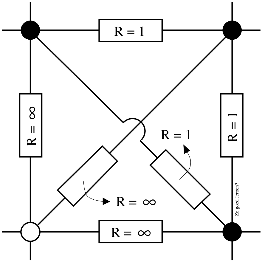
FIG. 1.: The assignment of resistors between neighbor and next-neighbor sites for the charge carriers with spin up. The small circles denote the lattice sites; black sites have a magnetization $S=+1$, white sites have $S=-1$. If both sites have $S=+1$ a unit resistance is put on the bond between them, otherwise the bond receives an infinite resistance. A similar assignment is made for the charge carriers with spin down.

The conductance of the model is calculated in the usual way: let $\Gamma$ be a configuration of magnetizations $S_{j}$ on the lattice sites. The conductance of this configuration can be calculated from the assignment of resistances, and is denoted by $\sigma(\Gamma)$. The expectation value of the overall conductance then is obtained by a weighted summation over all configurations in the usual way,

$\displaystyle\langle\sigma\rangle=\frac{1}{Z}\sum_{\Gamma}\sigma(\Gamma)\;\exp\big{(}-\beta H(\Gamma)\big{)},$

where $\beta=1/kT$, $Z$ is the partition function of the Ising model and $H(\Gamma)$ is the Hamiltonian of equation (1). We will now see what the predictions of this model are for the expectation value of the overall conductance of the lattice.

III The percolation phase diagram

The overall conductance of the lattice is defined as follows: consider a square lattice of $L\times L$ sites with resistances on bonds defined as in figure 1. Keep the lower row of the lattice at a fixed potential $V=0$ and the upper row at $V=1$. The conductance of the lattice is then equal to the expectation value of the current.

Conductance over the lattice is possible (e.g., non-zero) only if there exists a path from border to border exclusively over resistances $R=1$, that is, if at least one of the two spin directions is percolating[15, 16]. The qualitative features of the model thus can be obtained by considering the percolation phase diagram of the Ising model. In percolation, one defines clusters by putting bonds between neighbor spins $S=+1$ or $S=-1$. Let us consider percolation for sites $S=+1$; percolation for $S=-1$ is of course just the same but with the Ising magnetic field $h$ replaced by $-h$. In our case, a bond is placed between each pair of nearest and next-nearest neighbor sites having $S=+1$. These bonds make up clusters, and the percolation order parameter $P$ is the density of sites in the percolating cluster. If there is percolation then $P$ is finite, if there is no percolation, $P=0$.

Our case is called correlated percolation as the distribution of percolating ($S=+1$) and non-percolating ($S=-1$) sites is a correlated one. When this distribution is that of the Ising model, the phase diagram is known, and this is one of the reasons of choosing the Ising model as an example of our model: many exact results, also for percolation, are known for this model. Its percolation phase diagram is known[17] when percolating bonds are placed between each nearest neighbor pair of sites having $S=+1$. In another paper[18], we derive the phase diagram when next-nearest neighbor percolating bonds are defined as well. It is this phase diagram we need for our explanation; it is shown in figure 2.

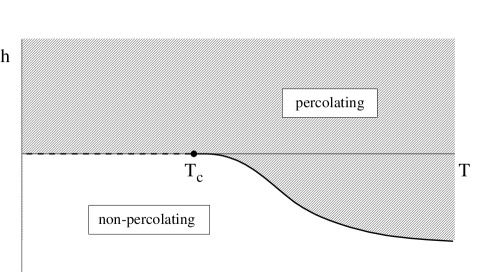
FIG. 2.: The percolation phase diagram for the Ising model for percolation of the up spins. Percolation is possible between nearest and next-nearest neighbor up spins. $T$ is temperature and $h$ is the magnetic field. The thick, solid line is a critical percolation line. The order parameter (the fraction of sites present in the largest cluster) is finite in the shaded area and goes continuously to zero when approaching the critical line. The critical line merges smoothly with the $T$-axis at $T_{c}$, which is a tricritical point for percolation. The dashed line is a first order transition for percolation, meaning that the order parameter jumps from a finite value to zero on this line.

In experiments, CMR occurs in thin films[3, 4, 5, 6] or even in bulk samples[2, 6, 10]. Our model thus should be pseudo three-dimensional or fully three-dimensional. This is the reason that in our two-dimensional model we defined resistances on next-nearest neighbor bonds as well. These ‘crossing’ bonds make the bond-graph non-planar, and this is the simplest way to mimic pseudo three-dimensional behavior. By defining these crossing bonds we allow for more possible paths between percolating sites, and the same is happening in a system consisting of several layers.

Inclusion of these crossing bonds is crucial, because without the crossing bonds there is no percolation[17] above the Curie temperature. At first it seems therefore that the percolation mechanism cannot explain the decreasing resistance above $T_{c}$. Inclusion of the crossing bonds, however, makes the region above $T_{c}$ percolating, and this is necessary for our explanation.

The effect of even more possible paths or of bonds with an even larger percolation range is, however, quite small. Even in a fully three-dimensional model, where there are many more possible paths for a cluster to follow, the percolation point lies only a few percent below the Curie temperature[19]. We expect, therefore, our conclusions also to hold in the case of a different lattice model or a different dimensionality. The percolation point may lie somewhat below $T_{c}$ but will be close to it. The phase diagram in that case is shown in figure 3.

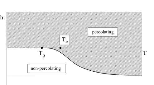
FIG. 3.: The phase diagram for a lattice model where the percolation point $T_{p}$ and the Curie point $T_{c}$ do not coincide. In this case the percolation temperature is always lower than the Curie temperature. The thick solid line is a critical percolation line in the universality class of random percolation and the same is expected for the endpoint of the line. The dashed line remains a first order transition line.

We choose to follow figure 2 for the explanation of our mechanism and the comparison with experiments. The qualitative comparison, however, holds for the other phase diagram of figure 3 as well.

For $T\rightarrow\infty$ or $K\rightarrow 0$ the probability distribution becomes a random one and the type of percolation is random percolation. The thick line merging smoothly with the $T$-axis is in the universality class of random percolation: on this line the order parameter vanishes algebraically with the same exponent as that for random percolation. The Curie point $T_{c}$ is the critical point of the Ising model, where there is a ferromagnetic-to-paramagnetic transition. For percolation, this point is a tricritical percolation point. The dashed line is a first order transition for the magnetization, and for percolation as well; the order parameter $P$ jumps from a finite value to zero over this line.

In principle, the percolation phase diagram tells nothing about the value of the conductance, only whether it is zero or non-zero. Nevertheless we may well assume that the closer one moves to the percolation threshold, the lower the conductance will be. From this, we can extract the qualitative behavior of the overall resistance from the phase diagram and draw a comparison with the experimental properties of CMR. To check the predictions of the phase diagram, we performed Monte Carlo calculations on the Ising resistor network. The results of these calculations confirm the predictions of the phase diagram, and are discussed in the next section.

Our conclusion is that the qualitative features of CMR are all present in the phase diagram of correlated percolation. Consider the following features:

1) The peak in the resistance at the Curie temperature $T_{c}$. According to the phase diagram, the only point on the $T$-axis where no percolation occurs for both spin directions is the Curie point $T_{c}$, so there is a peak in the resistance at $T_{c}$. (In fact, in our model this peak is infinitely high due to the choice $R=\infty$ on the insulating bonds.) All other points on the $T$-axis are percolating and hence show a better conductance.

2) The asymmetric shape of the peak in the resistance as a function of $T$. This shape is clearly present[2, 8, 9, 11] in experiments. In the phase diagram, moving away from $T_{c}$ is moving away from the percolation point and hence decreasing the resistance. Due to the presence of the critical percolation line that merges smoothly[17] with the $T$-axis, we expect this decrease to be slower above $T_{c}$, resulting in an asymmetric peak in the resistance. This expectation is confirmed using a Monte Carlo calculation, described in the next section.

3) The peak in the resistance as a function of magnetic field. In every experiment, the resistance peaks at zero field, a feature that is clearly present in the phase diagram. Moving away from the zero field axis means stimulating the percolation of one of the spin directions and hence decreasing the resistance. Note that our model does not give a correct numerical value of the magnetoresistance ratio $\Delta R/R$, where $\Delta R$ is the difference in resistance with and without magnetic field. What does follow from the model, however, is the qualitative result that this ratio is largest at $T_{c}$.

4) A particular observation in experiments is the shape of the peak in the resistance as a function of the magnetic field. As can be seen, e.g., from Fig. 1 in Ref. [5], Fig. 5 in Ref. [6], and Fig. 5 in Ref. [7], plots of the resistance versus the field display a cusp at temperatures below $T_{c}$ but are smooth at higher temperatures. This remarkable feature follows directly from the percolation phase diagram: below $T_{c}$ there is a first order transition line. Moving away from this line in both directions of the field immediately decreases the resistance, meaning that a plot of the resistance versus the field shows a cusp, the peak being strongest at $T_{c}$. Above $T_{c}$, on the other hand, there is no transition line at zero field, and hence the behavior of the resistance as a function of the magnetic field must be smooth.

5) It is observed[2, 6, 8, 11] in CMR that the peak in the resistance shifts to higher temperatures when a magnetic field is switched on. This directly follows from the presence of the percolation line in the phase diagram at temperatures above $T_{c}$. Switching on the magnetic field above $T_{c}$ one ‘feels’ the vicinity of this line, whereas below $T_{c}$ the nearest percolation point is $T_{c}$ itself, which is further away. Hence the resistance decreases more strongly as a function of the field below $T_{c}$.

This comparison shows that the basic features of CMR that are displayed in all experiments, are directly explained by our simple percolation mechanism. One single and simple mechanism accounts for its features, above as well as below the Curie temperature.

IV Resistance calculations

To make some predictions of our model, as explained in the previous section, more explicit, we performed Monte Carlo calculations on the Ising correlated resistor network. The model we used is that described in section II with the Hamiltonian of equation (1) and the assignment of resistors of figure 1.

We performed Monte Carlo simulations of the expectation value of the conductance for several lattice sizes. We used the Wolff-algorithm[20] for the Monte Carlo part, and the multigrid method of Edwards, Goodman and Sokal[21], based on the standard code amg1r4[22], to calculate the conductance of a spin configuration. The latter code is slightly changed, in order to cope with resistors on next-nearest neighbor bonds.

The interest in the first place is the behavior of the resistance for different temperatures. We performed calculations on different system sizes; the result is shown in figure 4. The peak in the resistance at $T_{c}$ becomes, for an infinite system, infinitely high, a result already following from the percolation phase diagram. The calculations confirm also the asymmetric shape of the peak in the resistance.

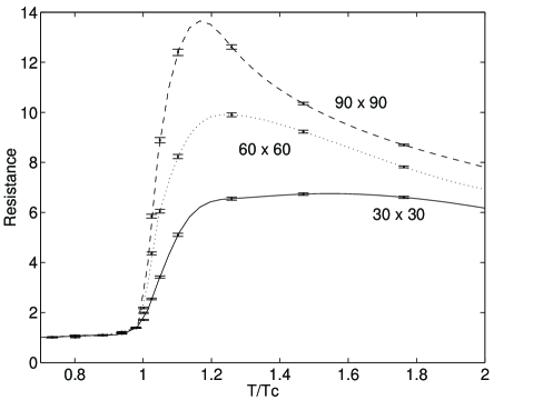
FIG. 4.: Resistance as a function of temperature for different system sizes at zero field. The system sizes are indicated in the plot, the resistance is scaled such that the minimal resistance (all bonds having $R=1$) is unity. The lines are guides to the eye. Resistors are defined as in figure 1. For larger systems, the peak shifts to $T_{c}$, becomes infinitely high but remains asymmetric. For $T<T_{c}$ there is a rapid convergence to the minimal (unit) resistance.

Secondly, the interest is in the critical exponents of the correlated resistor network. The interested reader is referred to reference [18] for a more detailed account. In this reference, we describe our calculations of the conductance exponent $t$ of the correlated resistor network. This exponent governs the algebraic decay of the conductance upon approaching a percolation threshold. Two different exponents play a role in the phase diagram of figure 2. The first is the exponent of the critical percolation line. It is defined as

$\displaystyle\sigma(h)\sim|h-h_{c}|^{t},$

where $\sigma(h)$ is the conductance at fixed $T>T_{c}$, and $h_{c}$ is the critical value of the magnetic field. The critical percolation line is in the universality class of random percolation, so the value of the exponent $t$ on this line must be that of the random resistor network. The random resistor network is a long standing unsolved problem in statistical physics, but good numerical results of the exponent $t$ are known. The best estimate[23] in two dimensions known to us is $t=1.299\pm 0.002$.

The second exponent involved is that governing the vanishing conductance at the Ising critical point. For percolation, this point is in a different universality class, and therefore the conductance exponent also differs from the random one. We calculated this exponent from the finite size behavior of the conductance, as explained in reference [18]. Because the Ising critical point is a tricritical point for percolation, there are two non-equivalent directions of approaching the critical point with two different exponents involved. For the temperature direction, the exponent $t$ is defined as

$$\sigma(T)\sim|T-T_{c}|^{t}\quad\text{at {\hbox{h=0}}},$$ (2)

yielding a value $t=0.2000\pm 0.0007$. For the other, field-like, direction, the exponent is defined as

$\displaystyle\sigma(h)\sim|h|^{t}\quad\text{for $T=T_{c}$}.$

In this case, the exponent $t$ has the value $t=0.1067\pm 0.0004$.

As will be explained in the next section, the numerical values of these exponents are of no direct interest, as the Ising model is not the correct lattice model for describing the CMR-materials. What is of interest, however, is the difference between the exponent of the critical line (random resistor network) and those of the Ising critical point (correlated resistor network). These exponents differ considerably. Even when there turns out to be no tricritical point in the correct phase diagram of the CMR-materials, as in figure 3, the model will, in a sense, be close to the tricritical point, which means that there will be an observable crossover from the random exponent to the value of the tricritical exponents.

V Discussion

We chose the Ising model to serve as an example for our mechanism for CMR, because of its simplicity and for the fact that many exact results are known for this model. There are, however, several features of our model that render it unrealistic for a more sophisticated explanation of CMR. The first is of course that the Ising model is not the appropriate lattice model, as the Ising variables $S_{j}$ do not have the symmetry of the CMR-materials. The latter are mostly perovskites, so the appropriate lattice model should have a magnetization vector $\bf m_{j}$ at each site $j$ that follows the symmetry of the perovskites.

A further shortcoming of our model is the infinite resistance for spin-up charge carriers on $(+-)$ and $(--)$ bonds. In principle, we should allow for a finite (but large) resistance on these bonds. The effect of this can be compared with the ferromagnetic-to-paramagnetic phase transition in the Ising model: if we switch on a small magnetic field, the true phase transition disappears, but the magnetization, specific heat and so on still show signs of the vicinity of the critical point. The same will happen when introducing these large but finite resistances. The actual value of this resistance displays the possibility of a spin-flip mechanism of the charge carriers. The importance of this effect is, we believe, quite small, such that the true phase transition is smeared out but the behavior of the overall resistance still shows signs of the vicinity of the percolation transition.

The finite height of the peak in the measurements can simply be incorporated by a large but finite ‘background’ resistance $R_{\infty}$ parallel to the net resistance of the correlated resistor network, representing the resistance of the ‘non-conducting’ bonds. The total resistance as a function of temperature $T$, following from equation (2), then becomes

$$R(T)=\frac{R_{\infty}}{1+a|T-T_{p}|^{t}},$$ (3)

where $T_{p}$ is the temperature where the resistance peaks, so $T_{p}$ is equal to or slightly lower than the Curie temperature $T_{c}$. The amplitude $a$ is non-universal and has in general different values above and below $T_{p}$.

Experiments so far have not been set up to measure critical exponents. For the exponent $t$ of equation (3), a rough analysis of the published data seems to point to a value between $1.5$ and $2.5$. It would be worthwhile to have more accurate experimental data on the exponents.

On the theoretical side, the interest is in the critical exponents of the correlated resistor network for the spin model corresponding to the magnetic anisotropy of the perovskites. Calculating these exponents is considerably more elaborate than in the Ising case, as even the percolation phase diagram has, to our knowledge, never been studied for models other than Ising.

VI Conclusions

We presented a correlated percolation mechanism for CMR and argued that its observed effects can be explained by considering the materials displaying CMR as a correlated resistor network. The introduced model only sheds light on the underlying mechanism, but is certainly not the appropriate one to reproduce accurate numerical results. For this, the model has to be changed into a spin model displaying the right magnetic anisotropy of the perovskites and has to be made pseudo or fully three-dimensional. Nevertheless, we argue, the qualitative results of the model will remain untouched.

- [1] Electronic address: paulb@tvs.kun.nl
- [2] Kusters R M, Singleton J, Keen D A, McGreevy R and Hayes W 1989 Physica B 155 362
- [3] Chahara K, Ohno T, Kasai M and Kozono Y 1993 Appl. Phys. Lett. 63 1990; Jin S, Tiefel T H, McCormack M, Fastnacht R A, Ramesh R and Chen L H 1994 Science 264 413
- [4] von Helmolt R, Wecker J, Holzapfel B, Schultz L and Samwer K 1993 Phys. Rev. Lett. 71 2331
- [5] McCormack M, Jin S, Tiefel T H, Fleming R M, Phillips J M and Ramesh R 1994 Appl. Phys. Lett. 64 3045
- [6] von Helmolt R, Wecker J, Samwer K, Haupt L and Bärner K 1994 J. Appl. Phys. 76 6925
- [7] Jin S, McCormack M, Tiefel T H and Ramesh R 1994 J. Appl. Phys. 76 6929
- [8] Schiffer P, Ramirez A P, Bao W and Cheong S-W 1995 Phys. Rev. Lett. 75 3336
- [9] Gong G-Q, Canedy C, Xiao G, Sun J Z, Gupta A and Gallagher W J 1995 Appl. Phys. Lett. 67 1783
- [10] Ju H L, Gopalakrishnan J, Peng J L, Li Q, Xiong G C, Venkatesan T and Greene R L 1995 Phys. Rev. B 51 6143
- [11] Shimakawa Y, Kubo Y and Manako T 1996 Nature 379 53
- [12] Zener C 1951 Phys. Rev. 82 403; de Gennes P-G 1960 Phys. Rev. 118 141
- [13] Pickett W E and Singh D J 1996 Phys. Rev. B 53 1146
- [14] de Boer P K, van Leuken H, de Groot R A, Barberis G E and Rojo T 1996 preprint
- [15] Essam J W 1972 in Phase Transitions and Critical Phenomena vol 2, ed. C Domb and M S Green (New York: Academic) p 218
- [16] Kirkpatrick S 1973 Rev. Mod. Phys. 45 574
- [17] Stella A L and Vanderzande C 1989 Phys. Rev. Lett. 62 1067
- [18] Bastiaansen P J M and Knops H J F 1996 preprint cond-mat/9610088
- [19] Müller-Krumbhaar H 1974 Phys. Lett. 50A 27
- [20] Wolff U 1989 Phys. Rev. Lett. 62 361
- [21] Edwards R G, Goodman J and Sokal A D 1988 Phys. Rev. Lett. 61 1333; Goodman J and Sokal A D 1989 Phys. Rev. D 40 2035
- [22] Ruge J and Stüben K 1987 in Multigrid Methods, ed. S F McCormick (Philadelphia: SIAM)
- [23] Normand J-M, Herrmann H J and Hajjar M 1988 J. Stat. Phys. 52 441