Storage capacity of correlated perceptrons

Abstract

We consider an ensemble of $K$ single-layer perceptrons exposed to random inputs and investigate the conditions under which the couplings of these perceptrons can be chosen such that prescribed correlations between the outputs occur. A general formalism is introduced using a multi-perceptron costfunction that allows to determine the maximal number of random inputs as a function of the desired values of the correlations. Replica-symmetric results for $K=2$ and $K=3$ are compared with properties of two-layer networks of tree-structure and fixed Boolean function between hidden units and output. The results show which correlations in the hidden layer of multi-layer neural networks are crucial for the value of the storage capacity.

1 Introduction

One of the central tasks in the field of statistical mechanics of neural networks is a deeper understanding of the information processing abilities of multi-layer feed-forward networks (MLN). After a thorough analysis of the single-layer perceptron it soon became clear that the very properties that entail the larger computational power of MLN also make their theoretical description within the framework of statistical mechanics much harder. Even the simplest case with just one hidden layer containing much less units than the input layer and with a pre-wired Boolean function from the hidden layer to the output has proven to be rather complicated to analyze exactly [3, 4, 5, 6]. It is therefore important to develop useful and reliable approximate methods to study these practically important systems. For the characterization of the generalization ability bounds for the performance parameters have been shown to yield useful orientations [7, 8]. For the storage capacity, i.e. the typical maximal number of random input-output mappings that can be implemented by the network only rather crude bounds exist so far, and these are independent of the hidden-to-output mapping ([9]).

Let us start the discussion with a number of general open questions regarding the capacity of MLN. These questions, although only partially answered in the present work, may serve as a call for further investigation by the community of the statistical mechanics of neural networks.

Correlations among the hidden units: The increased computational power of MLN stems from the possibility that the different subperceptrons between input and hidden layer can all operate in the region beyond their storage capacity. The occuring errors typical of this regime can be compensated by other subperceptrons. However, this “division of labour” only works appropriately if the errors do not occur for all subperceptrons in the same patterns. Hence intricate correlations depending on the hidden to output mapping develop in the hidden layer when the number of input-output pairs increases [14]. This qualitative picture has already been used to propose and analyze a learning algorithm for a special MLN, the parity-machine [15]. It has been observed for some time that the organization of internal representations described by these correlations is crucial for the understanding of the storage and generalization abilities of MLN [3, 10, 11, 12, 13].

The approximation suggested in this work is to replace “division of labour” by “average division of labour”. An approximate treatment of a MLN becomes possible if one does not require a definite mapping from the hidden layer to the output but instead prescribes the values for the correlations, i.e. the average relation between the hidden units and the output and also among the different hidden units themselves. The task is then to determine how many random inputs can be implemented by a set of $K$ perceptrons, such that the outputs show definite correlations.

Interplay between correlations and the capacity: This approach will highlight which type of correlations is easy to implement and which is difficult, i.e. reduce the storage capacity significantly. It is already known that increasing the average correlation between each one of the hidden units and the desired output decreases the capacity. This result can be examplified by the following well known limits. The lowest capacity is achieved for hidden units which are fully correlated with the desired outputs. In this case there is no division of labour and the MLN shrinks to a simple perceptron. The other limit is the parity machine, in which the correlation between each hidden unit and the output is zero. In this case the upper bound for the capacity of MLN with one hidden layer is achieved. Nevertheless, the general framework of how the capacity depends on the correlations between the output and a partial set of the hidden units is still unknown. The main problem is that with increasing $K$ there is a trade-off between a more flexible division of labour and an increasing complexity of possible correlations.

Possible scaling for the capacity: Of particular interest is the limit of an infinite number $K$ of hidden units for which only few analytical results are known. For the AND machine the capacity is of O(1) [10], whereas for the committee-machine and the parity machine the capacity is of order $(logK)^{\delta}$, with $\delta=1/2$ [13] and $1$ [4], respectively. These results may suggest one of the following two possible scenarios: In the first scenario, the capacity varies continuously as a function of the hidden/output correlations. Any $0\leq\delta\leq 1$ can be found, depending on the correlations. In the second possible scenario, $\delta=1$ holds for the parity machine only, and all other hidden/output correlations result in a $\delta$ with a finite distance from 1.

Space of possible correlations: The simmultaneous prescription of correlations involving several hidden units has to take into account that not all combinations of correlations are possible since they all derive from a common probability distribution. The question of whether there are forbidden combinations of correlations and what is their measure, will be partially answered in the following discussion.

The paper is organized as follows. Section 2 sets the task and fixes the notations. In section 3 the formalism is presented which is a generalization of the canonical phase space method developed by Gardner and Derrida [18] for the single–layer perceptron. Section 4 contains general results for an arbitrary number $K$ of perceptrons with a special subset of fixed correlations. In sections 5 and 6 we study in detail the situations of $K=2$ and $K=3$ perceptrons respectively and compare the results with those known for tree-structured MLN with the same number of hidden units. Finally, section 7 comprises our conclusions.

2 The storage problem for correlated perceptrons

We consider $K$ spherical perceptrons with $N/K$ inputs, one output, and couplings $\mathbf{J}_{k}\in I\!\!R^{N/K},\mathbf{J}_{k}\mathbf{J}_{k}=N/K$ with $k=1,\ldots,K$. Moreover we choose a set of $(\alpha N)K$ random inputs $\boldsymbol{\xi}_{k}^{\nu}\in I\!\!R^{N/K}$ and one overall random output $\sigma^{\nu}=\pm 1$ with $\nu=1,\ldots,\alpha N$. The total number of random input and output bits is hence $\alpha N(N+1)$ and the number of adjustable weights is $N$ as for the standard perceptron and for multilayer networks with tree-structure and fixed Boolean function between hidden units and output.

The outputs of the $K$ perceptrons are given by

$$\tau_{k}^{\nu}=\mbox{sgn}\left(\sqrt{\frac{K}{N}}\mathbf{J}_{k}\boldsymbol{\xi}_{k}^{\nu}\right)$$ (1)

Our aim is to determine the critical number $\alpha_{c}N$ of patterns for which coupling vectors $\mathbf{J}_{k}$ exist such that the averages

$$c_{1}=\langle\tau_{k}\sigma\rangle = \frac{1}{\alpha N}\sum_{\nu}\tau_{k}^{\nu}\sigma^{\nu}$$ (2)

$$c_{2}=\langle\tau_{k}\tau_{l}\sigma\rangle = \frac{1}{\alpha N}\sum_{\nu}\tau_{k}^{\nu}\tau_{l}^{\nu}\sigma^{\nu}$$

$$c_{3}=\langle\tau_{k}\tau_{l}\tau_{m}\sigma\rangle = \frac{1}{\alpha N}\sum_{\nu}\tau_{k}^{\nu}\tau_{l}^{\nu}\tau_{m}^{\nu}\sigma^{\nu}$$

$$\vdots$$

$$c_{K}=\langle\tau_{1}\cdots\tau_{K}\sigma\rangle = \frac{1}{\alpha N}\sum_{\nu}\tau_{1}^{\nu}\cdots\tau_{K}^{\nu}\sigma^{\nu}$$ (3)

have prescribed values $c_{1},c_{2},\cdots,c_{K}$. This can be seen as a generalization of the program of Gardner and Derrida [18] who considered only one perceptron, i.e. $K=1$, and determined $\alpha_{c}$ in dependence on the fraction of errors $f_{GD}$ related to $c_{1}$ by $c_{1}=1-2f_{GD}$. The new aspect of the present investigation is that not only the correlation of each individual output $\tau_{k}$ with $\sigma$ but also the correlation between different $\tau_{k}$ is taken into account.

As usual we assume that the components of the input patterns $\boldsymbol{\xi}_{k}^{\nu}$ as well as the overall outputs $\sigma^{\nu}$ are independent random variables with zero mean and unit variance. The transformation $\boldsymbol{\xi}_{k}^{\nu}\to\sigma^{\nu}\boldsymbol{\xi}_{k}^{\nu}$ then preserves the statistical properties of the inputs. In the following we therefore take $\sigma^{\nu}=1$ for all $\nu=1,\ldots,\alpha N$ without loss of generality.

Note that due to the independence of the inputs at different perceptrons all outputs $\tau_{k}$ have identical statistical properties. Therefore the correlations $c_{m}$ as defined in (2) do not depend on the particular subset of hidden units for which they are calculated. This corresponds to the permutation symmetry between hidden units in MLN with appropriate decoder functions ([4, 5, 6]).

It is in particular interesting to enforce correlations $c_{m}$ that are identical to those which develop spontaneously in MLN with special Boolean functions between hidden layer and output. It has recently been shown how these correlations can be calculated from the joint probability distribution of the stabilities at the hidden units [14]. For the parity machine with $K$ hidden units one finds $c_{m}=0$ for $m<K$ and $c_{K}=1$. For the committee machine the expressions are more complicated, for $K=3$ one finds $c_{1}=5/12,c_{2}=-1/6,c_{3}=-3/4$.

3 Formalism

To analyze the storage abilities of correlated perceptrons we use a generalization of the formalism introduced by Gardner and Derrida [18]. A well suited form for our purposes is the one proposed by Griniasty and Gutfreund [19]. We are hence led to introduce a multiperceptron cost function [20]

$$E(\mathbf{J}_{1},\cdots,\mathbf{J}_{K}) = \sum_{\nu}V(\tau^{\nu}_{1},\ldots,\tau^{\nu}_{K})$$ (4)

$$= \sum_{\nu}\left[-\sum_{k}\tau_{k}^{\nu}+\mu_{2}\sum_{(k,l)}\tau_{k}^{\nu}\tau_{l}^{\nu}+\mu_{3}\sum_{(k,l,m)}\tau_{k}^{\nu}\tau_{l}^{\nu}\tau_{m}^{\nu}+\cdots+\mu_{K}\>\tau_{1}^{\nu}\cdots\tau_{K}^{\nu}\right].$$ (5)

The parameters $\mu_{m}$ play the role of chemical potentials determining the costs for a violation of the constraints on the correlations $c_{m}$. Our aim is to characterize the coupling vectors $\mathbf{J}_{k}$ that minimize $E(\mathbf{J}_{1},\ldots,\mathbf{J}_{K})$ and to find the critical threshold $\alpha_{c}$ for the number of inputs for which no couplings $(\mathbf{J}_{1},\ldots,\mathbf{J}_{k})$ exist that realize the desired correlations. This can be done by calculating the free energy

$$f(\alpha,\beta,\mu_{2},\ldots,\mu_{K})=-\lim_{N\to\infty}\frac{1}{\beta N}\langle\langle\log\int\prod_{k=1}^{K}d{\mu}(\mathbf{J}_{k})\exp(-\beta E(\mathbf{J}_{1},\ldots,\mathbf{J}_{K})\rangle\rangle$$ (6)

where $\langle\langle\ldots\rangle\rangle$ denotes the quenched average over the inputs and $d\mu(\mathbf{J})=(2\pi e)^{-N/2K}\prod^{N/K}_{i=1}dJ_{i}\delta(\sum_{i=1}^{N/K}J_{i}^{2}-N/K)$ is the usual integration measure for spherical perceptrons. Then

$$g(\alpha_{c},\mu_{2},\ldots,\mu_{K})=\lim_{\beta\to\infty}f(\alpha,\beta,\mu_{2},\ldots,\mu_{K})$$ (7)

gives the typical minimum of $E(\mathbf{J}_{1},\ldots,\mathbf{J}_{K})$. The limit $\beta\to\infty$ corresponds to the saturation limit $\alpha\to\alpha_{c}$. The values $c^{(s)}_{m}$ of the correlations $c_{m}$ defined in eq.(2) in this saturation limit are from (4, 6) given by

$$\frac{1}{\alpha_{c}}g(\alpha_{c},\mu_{2},\cdots,\mu_{K}) = -Kc_{1}^{(s)}+\mu_{2}{K\choose 2}c_{2}^{(s)}+\cdots+\mu_{K}c_{K}^{(s)}$$ (8)

$$\frac{1}{\alpha_{c}}\frac{\partial g(\alpha_{c},\mu_{2},\cdots,\mu_{K})}{\partial\mu_{k}} = {K\choose k}c_{k}^{(s)}\qquad k=2,\cdots,K$$ (9)

Inverting these equations we find the saturation values $\alpha_{c}$ and $\mu_{m}^{(s)}$ as functions of $c_{1},\ldots,c_{K}$ which is what we were looking for.

The caluculation of $g(\alpha_{c},\mu_{2},\ldots,\mu_{K})$ proceeds along similar lines as for the single perceptron case studied in [19]. Within replica symmetry one has to introduce an order parameter $q$ characterizing the typical overlap between two coupling vectors that contribute significantly to the free energy (6). In the limit $\beta\to\infty$ it is convenient to replace this order parameter by $x=\beta(1-q)$. If the minimum of the costfunction is not degenrated we will find $q\to 1$ for $\beta\to\infty$ with $x$ remaining of order 1. Qualitatively $x$ describes the steepness of the minimum of the costfunction. The smaller $x$ the fewer couplings contribute significantly to the free energy for large $\beta$, i.e. the steeper the minimum of the costfunction. Accordingly $x=\infty$ correspondes to a degenerated minumum since $q\neq 1$ even for $\beta\to\infty$.

For all choices of the parameters $\mu_{m}$ there is a minimum $V_{min}=\min_{\{\tau_{k}\}}V(\tau_{1},\ldots,\tau_{K})$ of $V(\tau_{1},\ldots,\tau_{K})$ and hence $\alpha NV_{min}$ is a lower bound for the costfunction $E(\mathbf{J}_{1},\cdots,\mathbf{J}_{K})$. Now consider the subset of $\{\tau_{k}\}$-configurations that realize $V_{min}$ and calculate the correlations $c_{m}$ for this subset. The resulting values for the $c_{m}$ are special in two respects. First the value of $\alpha_{c}$ corresponding to them will occur for $x=\infty$ since the minimum of $E$ is degenerated for $\alpha<\alpha_{c}$. Second exactly these values of $c_{m}$ will occur in a MLN with that Boolean function between hidden layer and output that maps all the $\{\tau_{k}\}$-configurations that realize $V_{min}$ on the output $+1$. Consequently MLN with $K$ hidden units and fixed Boolean function between hidden layer and output will show up as “pure cases” defined by $x=\infty$ at $\alpha_{c}$ in our analysis and all situations with $x<\infty$ can be interpreted as these pure cases above saturation. Changing the parameters $\mu_{m}$ or equivalently the prescribed values of the $c_{m}$ will hence induce continuous transformations between the different possible MLN.

The main steps of the formal analysis are sketched in appendix A. The final result reads (cf. (34)(35))

$$g(\alpha_{c},\mu_{2},\cdots,\mu_{k})=-\min_{x}\left[\frac{1}{2x}-\alpha_{c}\int\prod_{k}Dt_{k}F(x,t_{k})\right]$$ (10)

where

$$F(x,t_{k})=\min_{\lambda_{1},\cdots,\lambda_{K}}\bigg{[}\frac{1}{2x}\sum_{k}(\lambda_{k}-t_{k})^{2}+V(\mbox{sgn}(\lambda_{1}),\ldots,\mbox{sgn}(\lambda_{K}))\bigg{]}$$ (11)

and $Dt=\exp(-t^{2}/2)dt/\sqrt{2\pi}$.

The minimization in (11) is non-trivial. The quadratic terms in (11) are smallest for $\lambda^{0}_{k}=t_{k}$. They compete with the step functions in $V(\mbox{sgn}(\lambda_{1}),\ldots,\mbox{sgn}(\lambda_{K}))$ giving rise to discontinous jumps in $F$ whenever one $\lambda_{k}$ crosses zero. Closer inspection shows that for the global minimum one has

$$\lambda^{0}_{k}=t_{k}\;\;{\textrm{o}r}\;\;\lambda^{0}_{k}=\bigg{\{}\begin{array}[]{lll}0^{+}&{\textrm{i}f}&t_{k}<0\\ 0^{-}&{\textrm{i}f}&t_{k}>0\end{array}$$ (12)

The saddlepoint equation which determines $x$ can be written in the form

$$\frac{1}{\alpha_{c}}=\int\prod_{k}Dt_{k}\sum_{k}(\lambda^{0}_{k}-t_{k})^{2}$$ (13)

Note that in this equation only those regions in the gaussian integrals contribute for which $\lambda_{k}^{0}\not=t_{k}$.

4 General results for prescribed highest and lowest correlation

Of particular interest is the case in which only the values of $c_{1}$ and $c_{K}$ are prescribed, i.e. $\mu_{2}=\mu_{3}=\ldots\mu_{K-1}=0$ in the costfunction (4). It describes the interpolation between individual perceptrons ($\mu_{K}=0$) and the parity machine ($\mu_{K}\to\pm\infty$) which is known to saturate the asymptotic upper bound $\alpha_{c}=\log K/\log 2$ for the storage capacity for large $K$ [4]. This special case is also sufficient to discuss the relation with the most important tree–structured MLN for $K=2$ and $K=3$. Moreover the necessary algebra simplifies somewhat.

Let us first note that the correlation coefficients $c_{1}$ and $c_{K}$ are not independent of each other. It is hence not possible to prescribe arbitrary values for them. According to their definition (2,3) we have always $c_{1},\;c_{K}\in(-1,+1)$. Moreover it is sufficient to consider positive values of $c_{1}$ only which is guarantied by the structure of the costfunction (4). Finally the relation

$$c_{K}\geq Kc_{1}-(K-1)$$ (14)

must hold. It is a consequence of the obvious observation that the difference between $c_{1}$ and $c_{K}$ is maximal if for every pattern at most one perceptron has negative output which corresponds to the equality sign in (14).

To perform the detailed analysis we denote $\mu_{K}$ simply by $\mu$ to get

$$E(\mathbf{J}_{1},\cdots,\mathbf{J}_{K}) = \sum_{\nu}\left[-\sum_{k}\tau_{k}^{\nu}+\mu\prod_{k}\tau_{k}^{\nu}\right].$$ (15)

Accordingly eq.(11) simplifies to

$$F(x,t_{k}) = \min_{\lambda_{1},\cdots,\lambda_{K}}\bigg{[}\frac{1}{2x}\sum_{k}(\lambda_{k}-t_{k})^{2}-\sum_{k}\mbox{sgn}(\lambda_{k})+\mu\>\mbox{sgn}(\lambda_{1}\lambda_{2}\cdots\lambda_{K})\bigg{]}.$$ (16)

In appendix B the following expressions for the correlation coefficients $c_{1}$ and $c_{K}$ are derived:

$$c_{1} = 1-2\>H(2\sqrt{x})\hskip 14.22636pt-\hskip 19.91684pt\bigg{[}f_{1}(|\mu|,x,0)-f_{2}(|\mu|,x,0)\bigg{]}$$ (17)

$$c_{K} = 2^{K}[1/2\>-\>H(2\sqrt{x})]^{K}-K{\rm sgn}(\mu)\bigg{[}f_{1}(|\mu|,x,0)+f_{2}(|\mu|,x,0)\bigg{]}$$ (18)

Moreover the saddlepoint equation fixing $x$ can be transformed into

$$\frac{1}{K\;\alpha_{c}}=\frac{1}{2}-H(2\sqrt{x})-2\sqrt{x}\frac{e^{-2x}}{\sqrt{2\pi}}+\frac{1}{2}\bigg{[}f_{1}(|\mu|,x,1)+f_{2}(|\mu|,x,1)\bigg{]}.$$ (19)

As usual we have used the abbreviation $H(x)=\int_{x}^{\infty}Dt$. $f_{1}(|\mu|,x,L)$ and $f_{2}(|\mu|,x,L)$ (with $L=0,1$) are integrals over sums of products of error functions explicitly given in appendix B. The final analysis of these equations has to be done numerically.

As discussed in the last section it is of particular interest to find the correlations $c_{1}$ and $c_{K}$ for which $x=\infty$ at $\alpha_{c}$. From eqs.(17)-(19) and (50)-(53) we find the following results

	$\mu$	$c_{1}(x=\infty)$	$c_{K}(x=\infty)$	$1/\alpha_{c}(x=\infty)$
I	$\mu<1$	1	1	K/2
II	$\mu=1$	$1-2/K+1/2^{(K-1)}K$	$-1+1/2^{(K-1)}$	$K/2-K\int\limits_{-\infty}^{0}Dt\;t^{2}\;[H(t)]^{K-1}$
III	$\mu>1$	$1-2/K$	$-1$	$K/2-K\int\limits_{0}^{\infty}Dt\;t^{2}\;\left([H(-t)]^{K-1}-[H(t)]^{K-1}\right)$

Table 1: Correlation coefficients and storage capacity for an ensemble of $K$ perceptrons in the pure cases characterized by $x=\infty$ (see text).

Note that all three pairs $(c_{1},c_{K})|_{(x=\infty)}$ lie on the line given by (14), in fact (I) and (III) are the endpoints of this line.

It is at first sight surprising that the parity machine does not occur in table (1). However from the structure of the cost-function (15) it is clear that the internal representations of the parity function realize $V_{min}$ only in the limit $\mu\to\pm\infty$. For finite $|\mu|$ the first term in (15) suppresses configurations with more than one negative output and gives rise to case (I) or (III).

5 $K=2$

The simplest case to apply the above concepts is provided by two perceptrons with $N/2$ inputs each corresponding to $K=2$. The only relevant correlations are $c_{1}$ and $c_{2}$ (see eqs.(2,3)). The relative importance of these in the cost-function (15) is regulated by $\mu$.

Solving (19) numerically for the case $K=2$ we find $c_{1}(\alpha_{c},\mu)$ and $c_{2}(\alpha_{c},\mu)$ from eqs.(17,18) and inverting these dependencies we arrive at $\alpha_{c}(c_{1},c_{2})$.

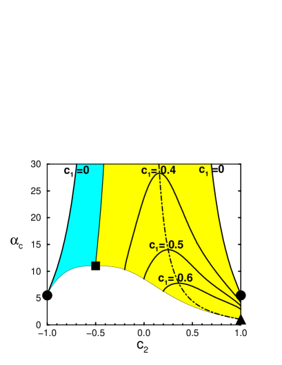
Figure 1: Storage capacity $\boldsymbol{\alpha}_{\mathbf{c}}\mathbf{(c_{1},c_{2})}$ for $\boldsymbol{K=2}$ correlated perceptrons. Left: $\alpha_{c}(c_{2})$ for $c_{1}=0,\;0.4,\;0.5$ and $0.6$. Outside the shaded areas no solutions exist, dark shade correspondes to $\mu>1$ light shade to $\mu<1$. The dashed-dotted line ($\mu=0$) gives the location of the maxima. The symbols denote the pure cases corresponding to the MLN summarized in table 2. Right: $\alpha_{c}(c_{1})$ for (from bottom to top): $c_{2}=1,\;0.8,\;0.7$, and $0.5$ (dashed) and $c_{2}=-0.8,\;-0.7$ and $-0.5$ (full). The lines end at the thin line given by $c_{2}=2c_{1}-1$. The symbol correspondes to the parity machine.

In fig.1(left) the dependence of $\alpha_{c}$ on $c_{2}$ for several values of $c_{1}$ is shown. Solutions exist only inside the shaded areas the boundaries of which correspond to $c_{1}=0$ and $c_{2}=2c_{1}-1$ respectively (cf.(14)). The maxima of $\alpha_{c}(c_{2})$ at constant $c_{1}$ occur for the uncorrelated system $\mu=0$ implying $c_{2}=c_{1}^{2}$ as expected since an additional constraint on $c_{2}$ can only reduce $\alpha_{c}$. The values of $\alpha_{c}(c_{1},c_{1}^{2})$ at these maxima are consistent with the results of Gardner and Derrida for the minimal fraction of errors $f_{GD}=(1-c_{1})/2$ [18].

Complementary the dependence $\alpha_{c}(c_{1})$ for fixed $c_{2}$ is shown in the right part of fig.1. Lines for $c_{2}$ and $-c_{2}$ start at the same point for $c_{1}=0$. It correspondes to $\mu=\pm\infty$ where the value of $c_{1}$ has negligible influence in the cost-function (15). With increasing $c_{1}$ the value of $\alpha_{c}$ always decreases because additional constraints are to be satisfied. These new constraints give rise to $c_{1}>0$ and are hence harder to satisfy for negative values of $c_{2}$. Finally all lines end at the thin line given by $c_{2}=2c_{1}-1$.

The pure cases for $K=2$ defined by $x=\infty$ at $\alpha_{c}$ are indicated by symbols in fig.1. They correspond to two-layer networks with two hidden units and fixed Boolean functions between hidden layer and output and are summarized in table 2.

symbol in fig.1	$c_{1}$	$c_{2}$	$\alpha_{c}(x=\infty)$	$\mu$	Boolean function
triangle	1	1	1	$<1$	AND
square	1/4	-1/2	11.01	$=1$	OR
circle	0	$-1$	5.50	$>1$	XOR

Table 2: Patterns of correlations for $K=2$ perceptrons equivalent to two-layer networks with fixed Boolean function between hidden units and output.

In our analysis the AND-machine denotes the situation in which the two perceptrons have to give simultaneously the correct output $\sigma^{\nu}=+1$ for all patterns. The storage capacity is hence given by the Gardner result, i.e. $\alpha_{c}=1$ since each perceptron has $N/2$ couplings only. Note that the AND-machine investigated in [10] has random outputs $\sigma^{\nu}=\pm 1$ and therefore the value for $\alpha_{c}$ is different. The XOR function defines the $K=2$ parity machine for which the replica symmetric $\alpha_{c}$ was first obtained in [3, 4]. The result for the OR-machine is new, again it refers to the situation where random inputs have all to be mapped on $\sigma^{\nu}=+1$. Finally let us note that there is another rather trivial pure case given by $c_{1}=c_{2}=0$ with $\alpha_{c}=\infty$ corresponding to the Boolean function that gives output $+1$ on any input.

The results obtained for $K=2$ are summarized in fig.2 showing the region of allowed values in the $c_{1}$-$c_{2}$-plane together with lines of constant $\alpha_{c}$ and constant $\mu$. The arrows at the lines of constant $\mu$ point to smaller values of $\alpha_{c}$. The above discussed hidden unit machines are again marked by the symbols of table2. All other points can be interpreted as these machines above their storage capacity. Note that the same point could be associated with different machines beyond saturation since by prescribing the correlations appropriately we can induce continuous transitions between different machines.

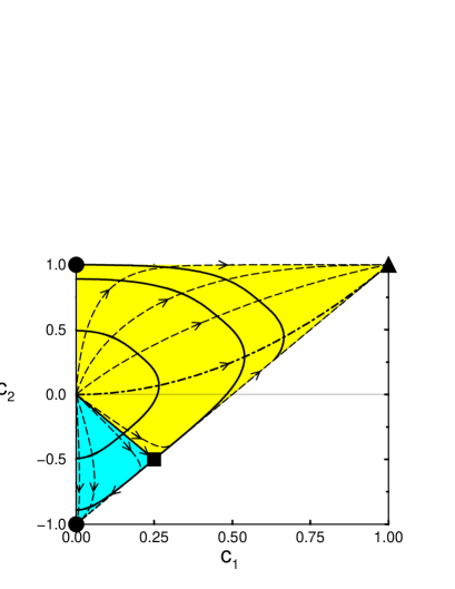
Figure 2: Contour map of $\boldsymbol{\alpha}_{\mathbf{c}}\mathbf{(c_{1},c_{2})}$ and $\boldsymbol{\mu}\mathbf{(c_{1},c_{2})}$ for $\mathbf{K=2}$ correlated perceptrons. Full lines correspond to $\alpha_{c}=100,11.01=\alpha^{OR}_{c},5.50=\alpha^{XOR}_{c}$ (from left to right), dashed lines to $\mu=-10,-2,-1,0,0.99,1.01,2$,and $10$ (from bottom to top). Symbols denote the same MLN as in table 2.

6 $K=3$

A similar analysis can be performed for $K=3$. As discussed in section 4 we set $\mu_{2}=0$ and denote $\mu_{3}$ simply by $\mu$. Similar to the last section we can than determine $\alpha_{c}(c_{1},c_{3})$ from a numerical analysis of eqs.(17,18).

Fig.3(left) shows the dependence of the critical storage capacity $\alpha_{c}$ on $c_{3}$ for fixed values of $c_{1}$. The dependencies are rather similar to the case $K=2$ shown in the left part of fig.1. Again solutions $c_{1}(\alpha_{c},c_{3})$ exist only in shaded areas. The maxima of the $\alpha_{c}(c_{3})$-curves lie on the dashed-dotted line corresponding to independent perceptrons ($\mu=0$). They are hence characterized by $c_{3}=c_{1}^{3}$ and are again consistent with the Gardner-Derrida results on the minimal fraction of errors for perceptrons above saturation [18].

Complementary the dependence $\alpha_{c}(c_{1})$ for fixed values of $c_{3}$ is shown in the right part of Fig.3. Again similar to the case $K=2$ we find that $\alpha_{c}$ decreases with increasing $c_{1}$. In particular the lines for $c_{3}=\pm 1$ show how the storage capacity decreases from the value of the $K=3$-parity machine at $c_{1}=0$ if additional constraints showing up in $c_{1}>0$ are included. All lines end at the thin line given by $c_{3}=3c_{1}-2$.

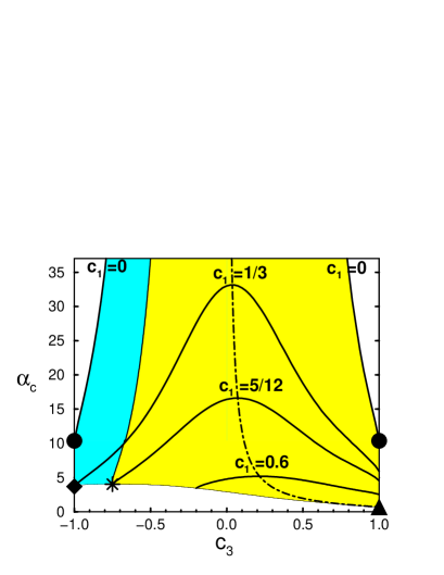
Figure 3: Storage capacity $\boldsymbol{\alpha}\mathbf{(c_{1},c_{3})}$ for $\mathbf{K=3}$ correlated perceptrons. Left: $\alpha_{c}(c_{3})$ for $c_{1}=0,1/3,5/12$ and $3/5$. Outside the shaded areas no solutions exist, dark shade correspondes to $\mu>1$ light shade to $\mu<1$. The dashed-dotted line ($\mu=0$) gives the location of the maxima. The symbols denote the pure cases corresponding to the MLN summarized in table 3. Right: $\alpha_{c}(c_{1})$ for (from bottom to top): $c_{3}=1,\;0.9$, and $0.5$ (dashed) and $c_{3}=-1,-.9$ and $-0.5$ (full). The lines end at the thin line given by $c_{3}=3c_{1}-2$. The symbol correspondes to the machine giving overall output $+1$ only if exactly one hidden unit is $-1$.

The symbols in fig.3 refer again to pure cases with $x=\infty$ at $\alpha_{c}$ corresponding to the MLN summarized in table 3. In addition to the and- and parity-machine we have now the committe-machine and a machine with the Boolean function for which the output is $+1$ if exactly one hidden unit is $-1$.

symbol in fig.(3)	$c_{1}$	$c_{3}$	$\alpha_{c}(x=\infty)$	$\mu$	Boolean function
triangle	1	1	2/3	$\mu<1$	AND
star	5/12	-3/4	4.02	$\mu=1$	COMMITTEE
diamond	1/3	-1	3.669	$\mu>1$	$(-\>+\>+),(+\>-\>+),(+\>+\>-)$
circle	0	$\pm 1$	10.37	$\mu=\pm\infty$	PARITY

Table 3: Patterns of correlations for $K=2$ perceptrons equivalent to two-layer networks with fixed Boolean function between hidden units and output.

We can again summarize the results in a contour plot showing lines of constant $\alpha_{c}$ and $\mu$ in the $c_{1}$-$c_{3}$-plane fig.4. Only combinations of $c_{1}$ and $c_{3}$ that belong to the shaded areas are possible, light shade correspondes to $\mu<1$, dark shade to $\mu>1$. The arrows at the dashed lines of constant $\mu$ point again into regions of lower $\alpha_{c}$, the symbols are those of table 3. Large values of $c_{1}$ imply a strong correlation of every perceptron with the common output and gives therefore small $\alpha_{c}$ and a narrow interval of consistent values of $c_{3}$. Relaxing the constraint on $c_{1}$ allows a more efficient “division of labour” between the perceptrons and results in a broader spectrum of $c_{3}$-values and enhanced storage capacity. Accordingly the largest values of $\alpha_{c}$ are possible for $c_{1}=0$. Then $\alpha_{c}$ only depends on $c_{3}$ and starting from the value $10.37$ for the parity machine at $c_{3}=\pm 1$ it increases without bound with decreasing $|c_{3}|$.

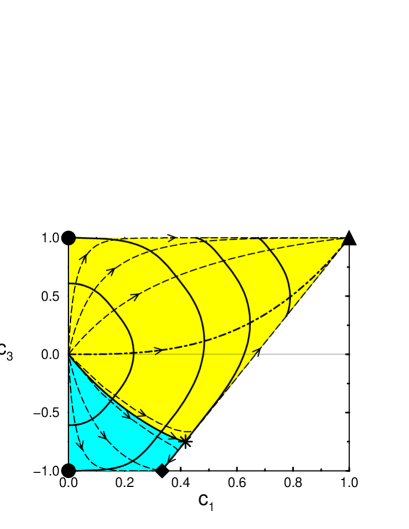
Figure 4: Contour map of $\boldsymbol{\alpha}_{\mathbf{c}}\mathbf{(c_{1},c_{3})}$ and $\boldsymbol{\mu}\mathbf{(c_{1},c_{3})}$ for $\mathbf{K=3}$ correlated perceptrons. Full lines correspond to $\alpha_{c}=100,10.37=\alpha_{c}^{PAR},4.02=\alpha_{c}^{COM}$ and 2. (from left to right), dashed lines to $\mu=-10,-2,-1,0,0.99,1.01,2$,and $10$ (from bottom to top). Symbols denote the same MLN as in table (3).

A new aspect of the case $K=3$ is that there is a correlation coefficient, $c_{2}$, that was not presribed (since we put $\mu_{2}=0$). It is nevertheless of interest to know the value of $c_{2}$ that correspondes to different choices of $c_{1}$ and $c_{3}$. The easiest way to obtain $c_{2}$ is via a maximum entropy argument. This is sketched in appendix C. The result is

$$c_{2}=-\frac{1}{2}+\sqrt{\frac{1}{4}+c_{1}^{2}+c_{1}c_{3}}$$ (20)

It is interesting to note that for the values $c_{1}=5/12$ and $c_{3}=-3/4$ characteristic for the committee-machine this formula gives $c_{2}=-1/6$ which is in fact the correct result [14]. The committee function for $K=3$ does hence not imply constraints on $c_{2}$ and is already uniquely characterized by the values of $c_{1}$ and $c_{3}$.

7 Conclusions

In the present paper we have considered ensembles of $K$ perceptrons with random inputs and investigated the possibility to choose the couplings such that prescribed correlations $c_{m}$ between the outputs of the perceptrons occur. For any combinatorically possible combination of $c_{m}$ there is a critical value $\alpha_{c}(c_{1},\ldots,c_{K})$ and solutions for the couplings of the perceptrons exist if the number of inputs is less than $N\alpha_{c}$. These investigation establish a relation between the results for single perceptrons above their storage capacity and those for several MLN with tree-structure and $K$ hidden units and fixed Boolean function between hidden layer and output. Similar ideas were persued in [15] and [11] where approximate expressions for the storage capacity of a parity machine and committee machine respectively were obtained from the results of Gardner and Derrida on the minimal fraction of errors of perceptrons beyond saturation and in [22] where analogies between a committee machine and noisy perceptrons were investigated. The new aspect in the present paper is that also the influence of higher correlations that are known to be important for the storage abilities was taken into account. The results show which correlations are difficult to implement and are therefore important for the determination of the storage capacity and which are easy and therefore not very restrictive. A detailed analysis was carried out for $K=2$ and $K=3$.

The technique used is a generalization of the canonical phase space analysis introduced by Gardner and Derrida. The results were obtained within the replica symmetric ansatz. They should hence be seen as a mere first orientation since it its well known that replica symmetry breaking (RSB) is crucial for both the description of perceptrons above saturation [21] and the storage abilities of MLN [4, 5, 6]. An investigation of the problem within RSB though highly desirable seems technically rather involved. Also the extension of the analysis to the asymptotic behaviour for $K\to\infty$ would be very interesting and would hopefully shed some light on the still controversial problem of the storage capacity of MLN in this limit.

Acknowledgement: We have benefitted from discussions with Chris van den Broeck and John Hertz. A.E. is grateful to the Minerva Center for Neural Networks for hospitality during a stay at BarIlan University in Ramat Gan where the initial stages of this work were performed.

8 Appendix A

In this appendix we outline the calculation of the free energy eq.(6) corresponding to the cost function eq.(4) within replica symmetry. To this end we employ a generalization of the formalism of Griniasty and Gutfreund [19].

To perform the average over the random patterns we use the replica trick

$$f(\mu_{2},...,\mu_{K},\beta) = -\frac{1}{\beta N}\langle\langle\ln{\cal Z}\rangle\rangle=-\frac{1}{\beta N}\lim\limits_{n\rightarrow 0}\frac{\langle\langle{\cal Z}^{n}\rangle\rangle-1}{n}$$ (21)

involving the partitition function ${\cal Z}$

$${\cal Z} = \int\limits_{-\infty}^{\infty}\prod\limits_{k}\frac{d\mathbf{J}_{k}}{\sqrt{2\pi e}}\delta(\mathbf{J}_{k}^{2}-N/K)\int_{-\infty}^{\infty}\prod\limits_{k\nu}d\lambda_{k}^{\nu}\delta(\lambda_{k}^{\nu}-\mathbf{J}_{k}\boldsymbol{\xi}_{k}^{\nu}\sqrt{K/N})e^{-\frac{\beta}{\alpha}\sum\limits_{\nu}^{\alpha N}V(\lambda_{1}^{\nu},...,\lambda_{K}^{\nu})}$$ (22)

$$V(\lambda^{\nu}_{1},...,\lambda^{\nu}_{K}) = -\sum_{k}{\rm sgn}(\lambda_{k}^{\nu})+\mu_{2}\sum_{(k,l)}{\rm sgn}(\lambda_{k}^{\nu}\lambda_{l}^{\nu})+\cdots+\mu_{K}{\rm sgn}(\lambda_{1}^{\mu}\cdots\lambda_{K}^{\mu})$$

Introducing integral representations for the $\delta$–functions and performing the average over the patterns we find

$$\langle\langle{\cal Z}^{n}\rangle\rangle = \int\limits_{-\infty}^{\infty}\prod\limits_{a<b;k}dq^{ab}_{k}\int\limits_{-\infty}^{\infty}\prod\limits_{a<b;k}dF^{ab}_{k}\frac{N}{2\pi K}\int\limits_{-\infty}^{\infty}\prod\limits_{a;k}\frac{dE^{a}_{k}}{4\pi K}$$ (23)

$$\times \exp\bigg{(}\frac{N}{K}\bigg{[}\frac{1}{2}\sum_{k}{\it tr}(Q_{k}A_{k})+G_{2}(F^{ab}_{k},E^{a}_{k})\bigg{]}+\alpha NG_{1}(Q_{1}..Q_{K})\bigg{)}$$

where

$$G_{2}(F^{ab}_{k},E^{a}_{k}) = -\frac{1}{2}\sum_{k}[n+{\rm tr}(\;\ln\;A_{k})],$$ (24)

and

$$\!\!\!\!G_{1}(Q_{1}..Q_{K})=\ln\bigg{[}\int\limits_{-\infty}^{\infty}\!\prod\limits_{k}d\boldsymbol{\lambda}_{k}\int\limits_{-\infty}^{\infty}\!\prod\limits_{k}\frac{d\mathbf{y}_{k}}{(2\pi)^{n}}\exp\bigg{(}i\sum\limits_{k}\mathbf{y}_{k}\boldsymbol{\lambda}_{k}-\frac{1}{2}\sum\limits_{k}\mathbf{y}_{k}Q_{k}\mathbf{y}^{T}_{k}+\beta\sum\limits_{a}V(\lambda^{a}_{1},...,\lambda^{a}_{K}\bigg{)}\bigg{]}$$ (25)

Here $\boldsymbol{\lambda}_{k}=(\lambda^{1}_{k},\cdots,\lambda^{n}_{k})$ and $\mathbf{y}_{k}=(y^{1}_{k},\cdots,y^{n}_{k})$ and we have used the matrices $Q_{k}$ and $A_{k}$:

$$Q_{k}=\bigg{(}\begin{array}[]{cc}1&q^{ab}_{k}\\ q^{ab}_{k}&1\end{array}\bigg{)}\hskip 14.22636pt,\hskip 14.22636ptA_{k}=\bigg{(}\begin{array}[]{cc}iE^{a}_{k}&-iF^{ab}_{k}\\ -iF^{ab}_{k}&iE^{a}_{k}\end{array}\bigg{)},$$ (30)

where as usual $q^{ab}_{k}$ describes the overlap between two replicas $a,\;b$ in the coupling space of perceptron $k$,

$$q^{ab}_{k}=\mathbf{J}^{a}_{k}\mathbf{J}^{b}_{k}K/N.$$ (31)

The saddlepoint for $E^{a}_{k}$ and $F^{ab}_{k}$ is given by $Q^{-1}_{k}=A_{k}$ resulting in

$$\langle\langle{\cal Z}^{n}\rangle\rangle\!\!\! \simeq \!\!\!\int\limits_{-\infty}^{\infty}\prod\limits_{a<b;k}dq^{ab}_{k}\exp\bigg{(}\frac{N}{2K}\sum_{k}\ln(\det\;Q_{k})+\alpha NG_{1}(Q_{1}..Q_{K})\bigg{)}$$ (32)

To evalute the remaining saddle point integral we use the replica symmetric ansatz $q^{ab}_{k}=q_{k}$ for all $a\neq b$. Moreover we expect permutation symmetry between the different perceptrons implying $q_{k}=q$ for all $k=1,..,K$. Then $\ln\>[\det Q]=n(\ln(1-q)+q/(1-q))$ and for $G_{1}(q_{1},..,q_{K})$ it follows

$$G_{1}(q)=$$ (33)

$$= \int\limits_{-\infty}^{\infty}\prod\limits_{a;k}d\lambda^{a}_{k}\int\limits_{-\infty}^{\infty}\prod\limits_{a;k}\frac{dy^{a}_{k}}{2\pi}\exp\bigg{(}i\sum\limits_{a;k}y^{a}_{k}\lambda^{a}_{k}-\frac{1-q}{2}\sum\limits_{a,k}(y^{a}_{k})^{2}-\frac{q}{2}\sum\limits_{a,k}(y^{a}_{k})^{2}-\beta V(\lambda^{a}_{1},...,\lambda^{a}_{K})\bigg{)}\bigg{]}$$

$$\simeq n\int\limits_{-\infty}^{\infty}\prod\limits_{k}Dt_{k}\;\ln\int\limits_{-\infty}^{\infty}\prod\limits_{k}\frac{d\lambda_{k}}{\sqrt{2\pi(1-q)}}\exp\bigg{(}-\sum_{k}\frac{(\lambda_{k}-t_{k}\sqrt{q})^{2}}{2(1-q)}-\beta V(\lambda_{1},...,\lambda_{K})\bigg{)}.$$

In order to calculate the function $g(\alpha_{c},\mu_{2},\ldots,\mu_{K})$ eq.(7) we have to consider the saturation limit $\beta\to\infty$. It is convenient then to use the rescaled saddle point variable $x=\beta(1-q)$ instead of $q$. In this way we obtain

$$g(\alpha_{c},\mu_{2},\ldots,\mu_{K}) = -\min\limits_{x}\bigg{[}\frac{1}{2x}-\alpha_{c}\int\limits_{-\infty}^{\infty}\prod\limits_{k}Dt_{k}F(x,t_{1},t_{2},...,t_{K})\bigg{]}$$ (34)

$$F(x,t_{1},t_{2},...,t_{K}) = \min\limits_{\lambda_{1},...,\lambda_{K}}\bigg{(}\sum_{k}\frac{(\lambda_{k}-t_{k})^{2}}{2x}+V(\lambda_{1},...,\lambda_{K})\bigg{)}$$ (35)

which coincides with (10). The saddlepoint equation eq.(13) determing $x$ follows by explicit differentiation of eq.(34) with respect to x.

9 Appendix B

In this appendix we sketch the main steps of the derivation of the saddle point equation (13) and of the free energy (34) for the case that only $c_{1}$ and $c_{K}$ are prescribed. We also give the explicit expressions for $c_{1}$ and $c_{K}$ as a function of $\alpha_{c}$ and $\mu$.

The calculation of g as given by (34,16) requires minimization of

$$F(x,t_{1},t_{2},...,t_{K})=\min\limits_{\lambda_{1},\lambda_{2},...\lambda_{K}}\bigg{[}\sum_{k=1}^{K}\frac{(\lambda_{k}-t_{k})^{2}}{2x}-\sum_{k=1}^{K}{\rm sign}(\lambda_{k})+\mu\prod_{k=1}^{K}{\rm sign}(\lambda_{k})\bigg{]}.$$ (36)

From eq.(12) we have

$${\rm sgn}(\lambda^{0}_{k})=\bigg{\{}\begin{array}[]{rc}\;\;\;{\rm sgn}(t_{k})&{\rm if}\hskip 5.69046pt\lambda^{0}_{k}=t_{k}\\ -{\rm sgn}(t_{k})&{\rm else}\end{array}$$ (39)

Eq.(36) then becomes

$$F(x,t_{1},t_{2},...,t_{K})=\bigg{[}\mu\;S(\vec{\lambda^{0}})-\sum_{k=1}^{K}{\rm sgn}(t_{k})+\sum_{\forall_{j}\lambda^{0}_{j}=0^{\pm}}\bigg{(}\frac{t_{j}^{2}}{2x}+2\;{\rm sgn}\>t_{j}\bigg{)}\bigg{]}.$$ (40)

Here $S(\vec{\lambda^{0}})=\prod_{k=1}^{K}{\rm sgn}(\lambda_{k}^{0})=(-1)^{m}\prod_{k=1}^{K}{\rm sgn}(t_{k})$ were $m$ counts all $\lambda^{0}_{k}\equiv 0$. The last sum in eq.(40) has only contributions from those $\lambda$ with $\lambda^{0}_{j}=0^{\pm}$.

To minimize $F$ for given $t_{1},...,t_{K}$ we have hence to find which of the $2^{K}$ configurations $\{\lambda_{1}^{0},...,\lambda_{K}^{0}\}$ , $\lambda^{0}_{k}=\{0^{\pm},t_{k}\}$, minimizes eq.(40). A suitable procedure to do this is as follows. We first make the last term in eq.(40) as small as possible. That is for all $t_{j}$ with $t_{j}\in(-2\sqrt{x},0)$ we choose for a first try $\lambda^{0}_{j}=0^{\pm}$. We denote the resulting value for $S(\vec{\lambda^{0}})$ by $S^{*}$. ($S^{*}=(-1)^{\eta}$ where $\eta$ is the number of all $t_{k}<-2\sqrt{x}$.) If $\mu\;S^{*}(\vec{t})<0$ the optimal configuration has already been found because the first summand is at its miminum as well. If on the other hand $\mu\;S^{*}(\vec{t})>0$ there is competition between the first and the last term in eq.(40). One may then change the sign of $S(\vec{\lambda^{0}})$ in order to lower $F(x,t_{1},t_{2},...,t_{K})$ by $2|\mu|$ by either setting a single $\lambda_{l}^{0}=0^{\pm}$ althought $t_{l}\not\in(-2\sqrt{x},0)$ or setting a single $\lambda_{l}^{0}=t_{l}$ for one $t_{l}\in(-2\sqrt{x},0)$. The corresponding changes in $F$ are $2(w(t_{l})-|\mu|)$ where

$$w(t)=\left\{\begin{array}[]{r l}t^{2}/4x\;\;-\;\;1&\;\;{\rm if}\hskip 8.5359ptt\in(-\infty,-2\sqrt{x})\\ -t^{2}/4x\;\;+\;\;1&\;\;{\rm if}\hskip 8.5359ptt\in(-2\sqrt{x},0)\\ t^{2}/4x\;\;+\;\;1&\;\;{\rm if}\hskip 8.5359ptt\in(0,\infty)\end{array}\right..$$ (44)

To the saddle point equation (13) only regions in the integral contribute for which $\lambda_{j}^{0}\neq t_{j}$ for at least one $j$. Formalizing the above consideration we find

$$\frac{1}{\alpha_{c}} = \int\limits_{-\infty}^{\infty}\!...\int\limits_{-\infty}^{\infty}Dt_{1}...Dt_{K}\bigg{\{}\sum_{k=1}^{K}t_{k=1}^{2}\Theta_{I}(t_{k})+$$ (45)

$$+ K\Theta(\mu\;S^{*})\Theta(|\mu|-w(t_{1}))t_{1}^{2}(-1)^{\Theta_{I}(t_{1})}\prod_{k=2}^{K}\Theta(w(t_{k})-w(t_{1}))\bigg{\}}$$

$$\Theta_{I}(t) = \bigg{\{}\begin{array}[]{cc}1&{\rm if}\hskip 5.69046ptt\in(-2\sqrt{x},0)\\ 0&{\rm else}\end{array}$$ (48)

The first term of eq.(45) stems from our first guess minimizing the last term of eq.(40) only. The various Theta–functions in the term that contributes only for $\mu\;S^{*}>0$ implement the different cases discussed in context with eq.(44). Integration variables can be renamed that always $t_{1}<t_{2}<\cdots<t_{K}$ with no restriction of generality.

The integrations over $t_{2},...,t_{K}$ yields a product of sums of two error functions. Finally the saddlepoint equation reads

$$\frac{1}{K\;\alpha_{c}}=\frac{1}{2}-H(2\sqrt{x})-2\sqrt{x}\frac{e^{-2x}}{\sqrt{2\pi}}+\frac{1}{2}\bigg{[}f_{1}(|\mu|,x,1)+f_{2}(|\mu|,x,1)\bigg{]}.$$ (49)

$$f_{1}(|\mu|<1,x,L)=[-1]^{L}\int\limits_{-2\sqrt{x}}^{-2\sqrt{x(1-|\mu|)}}Dt_{1}\>t_{1}^{2L}\bigg{(}\bigg{[}H(t_{1})+H_{m}(t_{1})\bigg{]}^{K-1}\!\!\!\!\!\!\!\!\!+{\rm sgn}\mu\bigg{[}H(t_{1})-H_{m}(t_{1})\bigg{]}^{K-1}\bigg{)}$$ (50)

$$f_{1}(|\mu|>1,x,L) = \bigg{\{}\hskip 8.5359pt\int\limits_{0}^{2\sqrt{x(|\mu|-1)}}Dt_{1}\>t_{1}^{2L}\bigg{(}\bigg{[}H(t_{1})+H_{p}(t_{1})\bigg{]}^{K-1}\!\!\!\!\!\!\!\!\!+{\rm sgn}\mu\bigg{[}H(t_{1})-H_{p}(t_{1})\bigg{]}^{K-1}\bigg{)}+$$ (51)

$$[-1]^{L}\int\limits_{-2\sqrt{x}}^{0}\!Dt_{1}\>t_{1}^{2L}\bigg{(}\bigg{[}H(t_{1})+H_{m}(t_{1})\bigg{]}^{K-1}\!\!\!\!\!\!\!\!\!+{\rm sgn}\mu\bigg{[}H(t_{1})-H_{m}(t_{1})\bigg{]}^{K-1}\bigg{)}\bigg{\}}$$

where we introduced the abbreviation $H_{p}(t_{1})=H(\sqrt{8x+t_{1}^{2}})$, $H_{m}(t_{1})=H(\sqrt{|8x-t_{1}^{2}|})$ and $H^{-}_{m}(t_{1})=H(-\sqrt{|8x-t_{1}^{2}|})$. As usual $H(t)=\int\limits_{t}^{\infty}Dt$. Similarly

$$f_{2}(|\mu|<1,x,L)=\int\limits_{-2\sqrt{x(1+|\mu|)}}^{-2\sqrt{x}}Dt_{1}\>t_{1}^{2L}\bigg{(}\bigg{[}H^{-}_{m}(t_{1})+H(-t_{1})\bigg{]}^{K-1}\!\!\!\!\!\!\!\!\!-{\rm sgn}\mu\bigg{[}H^{-}_{m}(t_{1})-H(-t_{1})\bigg{]}^{K-1}\bigg{)}$$ (52)

$$f_{2}(|\mu|>1,x,L) = \bigg{\{}\int\limits_{-2\sqrt{2x}}^{-2\sqrt{x}}Dt_{1}\>t_{1}^{2L}\bigg{(}\bigg{[}H^{-}_{m}(t_{1})+H(-t_{1})\bigg{]}^{K-1}\!\!\!\!\!\!\!\!\!-{\rm sgn}\mu\bigg{[}H^{-}_{m}(t_{1})-H(-t_{1})\bigg{]}^{K-1}\bigg{)}$$ (53)

$$+\int\limits_{-2\sqrt{x(1+|\mu|)}}^{-2\sqrt{2x}}Dt_{1}\>t_{1}^{2L}\bigg{(}\bigg{[}H_{m}(t_{1})+H(-t_{1}))\bigg{]}^{K-1}\!\!\!\!\!\!\!\!\!-{\rm sgn}\mu\bigg{[}H_{m}(t_{1})-H(-t_{1}))\bigg{]}^{K-1}\bigg{)}\bigg{\}}$$

A common feature of eq.(50–53) is that in the binomial expression those terms cancel which correspond to regions with $\mu S^{*}<0$.

The calculation of $g$ proceedes along similar lines.

$$g/\alpha_{c} = \int\limits_{-\infty}^{\infty}\!...\int\limits_{-\infty}^{\infty}Dt_{1}...Dt_{K}\bigg{\{}\mu\;S^{*}-\sum_{k=1}^{K}{\rm sgn}(t_{k})+2\sum_{\forall_{j}\lambda^{0}_{j}=0}{\rm sgn}\>t_{j}\bigg{\}}$$ (54)

$$= \int\limits_{-\infty}^{\infty}\!...\int\limits_{-\infty}^{\infty}Dt_{1}...Dt_{K}\bigg{\{}\mu\;S^{*}-2\sum_{k=1}^{K}\Theta_{I}(t_{k})+2K\Theta(\mu\;S^{*})\Theta(|\mu|-w(t_{1}))\times$$

$$\times\bigg{(}-\mu\;S^{*}+(-1)^{\Theta_{I}(t_{1})}{\rm sgn}(t_{1})\bigg{)}\prod_{k=2}^{K}\Theta(w(t_{k})-w(t_{1}))\bigg{\}}$$

We find

$$g/\alpha_{c} = -2K\>E(2\sqrt{x})+2^{K}\mu E^{K}(2\sqrt{x})+$$ (55)

$$+ K\bigg{\{}f_{1}(|\mu|,x,0)-f_{2}(|\mu|,x,0)-|\mu|\bigg{[}f_{1}(|\mu|,x,0)+f_{2}(|\mu|,x,0)\bigg{]}\bigg{\}}$$

Performing the derivative of $g/\alpha_{c}$ with respect to $\mu$ one realizes that there is no contribution from the $\mu$–dependence of the integration limits in eqs.(50–53). Hence the expression (55) for $g/\alpha_{c}$ is already of the form $g/\alpha_{c}=-Kc_{1}\;+\;\mu\;c_{K}$ und we arrive at eq.(17,18) for the correlation coefficients $c_{1}$ and $c_{K}$.

10 Appendix C

To determine $c_{2}$ for given values of $c_{1}$ and $c_{3}$ we look for the probability distribution $P(\tau_{1},\tau_{2},\tau_{3})$ that for the given values of $c_{1}$ and $c_{3}$ realizes the maximal entropy. Because of the permutation symmetry between the perceptrons we have only to determine the probabilities $p_{k}$ of output configurations with $k$ negative outputs where $k=0,\ldots,3$. Hence we have to maximize

$$S = -p_{0}\log p_{0}-3p_{1}\log p_{1}-3p_{2}\log p_{2}-p_{3}\log p_{3}$$

$$+\lambda_{0}(p_{0}+3p_{1}+3p_{2}+p_{3}-1)$$

$$+\lambda_{1}(p_{0}+p_{1}-p_{2}-p_{3}-c_{1})$$

$$+\lambda_{3}(p_{0}-3p_{1}+3p_{2}-p_{3}-c_{3})$$

where the $\lambda_{k}$ are Lagrange multiplier incorporating the constraints. Performing the derivatives with respect to the $p_{k}$ yields

$$p_{0}p_{3}=p_{1}p_{2}$$ (57)

Using the constraints to solve for the $p_{k}$ gives

$$c_{2}=-\frac{1}{2}\pm\sqrt{\frac{1}{4}+c_{1}^{2}+c_{1}c_{3}}$$ (58)

where only the upper sign give rise to positive values for all $p_{k}$.

References

- [1] J. A. Hertz, A. Krogh, and R. G. Palmer, Introduction to the theory of neural computation, (Addison-Wesley, Redwood City, 1991)
- [2] D. E. Rummelhart and J. E. McClelland (eds.) Parallel Distributed Processing, (MIT Press, Cambridge, MA, 1986)
- [3] M. Mezard and S. Patarnello, On the Capacity of Feedforward Layered Networks, LPTENS-preprint 1989, unpublished
- [4] E. Barkai, D. Hansel, and I. Kanter, Phys. Rev. Lett. 65, 2312 (1990)
- [5] E. Barkai, D. Hansel, and H. Sompolinsky, Phys. Rev. A45, 4146 (1992)
- [6] A. Engel, H. M. Koehler, F. Tschepke, H. Vollmayr, and A. Zippelius, Phys. Rev. A45, 7590 (1992)
- [7] D. Haussler, M. Kearns, and R. Schapire, Bounds on the Sample Complexity of Bayesian Learning Using Information Theory and the VC Dimension, Proceedings COLT ’91, Morgan Kaufmann, San Mateo.
- [8] M. Opper, Phys. Rev.E51, 3613 (1995)
- [9] G. J. Mitchison and R. M. Durbin, Biol. Cybern. 60, 345 (1989)
- [10] M. Griniasty and T. Grossman, Phys. Rev. A45, 8924 (1992)
- [11] A. Priel, M. Blatt, T. Grossman, E. Domany, and I. Kanter, Phys. Rev. E50, 577 (1994)
- [12] B. Schottky, J. Phys. A28, 4515 (1995)
- [13] R. Monasson and R. Zecchina, Phys. Rev. Lett. 75, 2432 (1995)
- [14] A. Engel J. Phys. A29, L323 (1996)
- [15] M Biehl and M. Opper, Phys. Rev. A44, 6888 (1991)
- [16] G. Cybenko, Math. Control Signals Systems 2, 303 (1989)
- [17] D. Saad and S. Solla, Phys. Rev. Lett. 74, 4337 (1995)
- [18] E. Gardner and B. Derrida, J. Phys. A21, 271 (1988)
- [19] M. Griniasty and H. Gutfreund, J. Phys. A24, 715 (1991)
- [20] The application of this technique to a single perceptrons has been extensively investigated in M. Bouten, J. Schietse, and C. van den Broeck, Phys. Rev. E52, 1958 (1995)
- [21] M. Bouten J. Phys. A27, 6021 (1994)
- [22] M. Copelli, O. Kinouchi, and N. Caticha, Phys. Rev. E53, 6341 (1996)