Effect of the coupling to a superconductor
on the level statistics of a metal grain in a magnetic field

Abstract

A theory is presented for the statistics of the excitation spectrum of a disordered metal grain in contact with a superconductor. A magnetic field is applied to fully break time-reversal symmetry in the grain. Still, an excitation gap of the order of $\delta$ opens up provided $N\Gamma^{2}\gtrsim 1$. Here $\delta$ is the mean level spacing in the grain, $\Gamma$ the tunnel probability through the contact with the superconductor, and $N$ the number of transverse modes in the contact region. This provides a microscopic justification for the new random-matrix ensemble of Altland and Zirnbauer.

PACS numbers: 74.50.+r, 74.80.Fp, 05.45.+b

The proximity to a superconductor is known to induce a gap in the excitation spectrum of a normal metal. Semiclassical theories of this “proximity effect” show that the gap closes if time-reversal symmetry (${\cal T}$) is broken (by a magnetic field or by magnetic impurities). Recently, Altland and Zirnbauer [1] argued that a gap remains in the spectrum of a metal grain surrounded by a superconductor — even if ${\cal T}$ is broken completely. (The classical mechanics of such a system had previously been studied [2].) The gap is small (of the order of the mean level spacing in the grain), but it has the fundamental implication that the level statistics is no longer described by the Gaussian unitary ensemble (GUE) of random-matrix theory [3].

The GUE has a probability distribution of energy levels of the form

$$P(\{E_{n}\})\propto\prod_{i<j}(E_{i}-E_{j})^{2}\prod_{k}\exp\left(-cE_{k}^{2}\right),$$ (1)

with some constant $c>0$ depending on the mean level spacing at the Fermi level (chosen at $E=0$). This ensemble was first applied to a granular metal by Gorkov and Eliashberg [4], and derived from microscopic theory by Efetov many years later [5]. A single-particle energy level $E_{n}$ corresponds to an excitation energy $|E_{n}|$, that is to say, the excitation spectrum is obtained by folding the single-particle spectrum along the Fermi level. The folded GUE has been studied in Ref. [6]. Altland and Zirnbauer introduce a different probability distribution,

$$P(\{E_{n}\})\propto\prod_{i<j}(E_{i}^{2}-E_{j}^{2})^{2}\prod_{k}E_{k}^{2}\,\exp\left(-2cE_{k}^{2}\right),$$ (2)

for the (positive) excitation energies of a metal grain in contact with a superconductor. (The excitation spectrum is discrete for $E<\Delta$, with $\Delta$ the excitation gap in the bulk of the superconductor.) The distribution (2) is related to the Laguerre unitary ensemble (LUE) of random-matrix theory [7] by a change of variables. The density of states $\rho(E)$ in this ensemble vanishes quadratically near zero energy [1, 7],

$$\rho(E)=\frac{1}{\delta}\left(1-\frac{\sin(2\pi E/\delta)}{2\pi E/\delta}\right).$$ (3)

The gap in the excitation spectrum is of the order of the mean level spacing $\delta$. The folded GUE, on the contrary, has no gap but a constant $\rho(E)=1/\delta$ near $E=0$.

In this paper we present the first microscopic theory for the effect on the level statistics of the coupling to a superconductor. We consider the case that the conventional proximity effect is fully destroyed by a ${\cal T}$-breaking magnetic field [8]. Assuming non-interacting quasiparticle excitations, and starting from the well-established GUE for the level statistics of an isolated metal grain, we obtain a crossover to Altland and Zirnbauer’s distribution (2) as the coupling to a superconductor is increased. This provides a microscopic justification for the “maximum-entropy” hypothesis on which Ref. [1] was based. Such a justification is needed because, in contrast to ensembles in statistical mechanics, there is no physical principle that would require a random-matrix ensemble to maximize entropy. Furthermore, because the argument of Ref. [1] is based on the presence or absence of a certain discrete symmetry in the Hamiltonian, it can not provide a criterion for how strong the coupling to the superconductor should be for the new ensemble to apply. Our microscopic approach permits us to identify this criterion, and to compute explicitly how the gap in $\rho(E)$ opens up as the coupling strength is increased.

We consider the geometry shown in Fig. 1 of a disordered metal grain (N), which is connected to a superconductor (S) by a point contact or microbridge containing a tunnel barrier. Breaking ${\cal T}$ requires a magnetic field of at most a flux quantum through the grain. This field is less than the critical field of the superconductor if the size of the grain is greater than the superconducting coherence length. For simplicity of presentation we consider a real order parameter $\Delta$ in S. (We have found that a spatial dependence of the superconducting phase, considered in Ref. [1], has no effect on the level statistics in the absence of ${\cal T}$.) We assume zero temperature, so that motion in the grain is totally phase coherent. We seek the distribution of the excitation energies $E_{n}\ll\Delta$. We first consider the density of states $\rho(E)$.

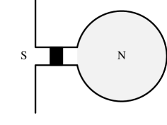
FIG. 1.: A disordered normal-metal grain (N) coupled to a superconductor (S). The black area indicates a tunnel barrier.

To determine $\rho(E)$ we adopt the scattering approach of Ref. [9]. We model the point contact by a normal-metal lead supporting $N$ transverse modes at the Fermi level. Andreev reflection at the interface scatters electrons into holes. This corresponds to the off-diagonal blocks in the scattering matrix $S_{\rm A}$ for Andreev reflection,

$$S_{\rm A}=\left(\begin{array}[]{cc}0&-i\\ -i&0\\ \end{array}\right),$$ (4)

where each of the four blocks is an $N\times N$ matrix. The scattering matrix $S_{\rm N}$ for the normal-metal grain plus tunnel barrier does not couple electrons and holes, and thus has the block diagonal form

$$S_{\rm N}=\left(\begin{array}[]{cc}S_{0}(E)&0\\ 0&S_{0}^{*}(-E)\end{array}\right).$$ (5)

Here $S_{0}$ ($S_{0}^{*}$) is the scattering matrix for electrons (holes) at an energy $E$ from the Fermi level. The $N\times N$ scattering matrix $S_{0}$ can be expressed in terms of the $M\times M$ Hamiltonian $H_{0}$ of the isolated grain and an $M\times N$ coupling matrix $W$ [10, 11]:

$$S_{0}(E)=1-2\pi iW^{\dagger}(E-H_{0}+i\pi WW^{\dagger})^{-1}W.$$ (6)

The finite dimension $M$ of $H_{0}$ is artificial and will be taken to infinity later on.

As demonstrated by Efetov [5], an ensemble of disordered metal grains in a magnetic field can be described by the GUE [12],

$$P(H_{0})\propto\exp\left(-c\,\mbox{Tr}\,H_{0}^{2}\right).$$ (7)

(Eq. (1) follows upon integration over the eigenvectors of $H_{0}$.) The coefficient $c$ is related to $\delta$ by $c=\pi^{2}/8M\delta^{2}$. We recall that $\delta$ is the mean level spacing in the folded GUE, which is one half the mean level spacing of $H_{0}$. The coupling matrix $W$ has the form [11, 13]

$$W_{mn} = \delta_{mn}\left(\frac{2M\delta}{\pi^{2}}\right)^{1/2}\!\!\left(2\Gamma_{n}^{-1}-1+2\Gamma_{n}^{-1}\sqrt{1-\Gamma_{n}}\right)^{1/2},$$ (9)

$$m=1,2,\ldots,M,\quad n=1,2,\ldots,N.$$

Here $\Gamma_{n}$ is the tunnel probability of mode $n$ through the normal lead [14]. For later use we introduce a parameter $\lambda=2M\delta/\pi$ and an $M\times M$ matrix $X=(\pi/\lambda)WW^{\rm T}$. In view of Eq. (9), the matrix $X$ is diagonal with $N$ non-zero diagonal elements $x_{n}$, related to $\Gamma_{n}$ by

$$\Gamma_{n}=4x_{n}\,(1+x_{n})^{-2}.$$ (10)

The excitation energies $E_{n}$ are the positive roots of the equation Det$[1-S_{\rm A}\,S_{\rm N}(E)]=0$, which can be rewritten as an eigenvalue equation [15],

$$\mbox{Det}(E-{\cal H})=0,\quad{\cal H}=\left(\begin{array}[]{cc}H_{0}&-\lambda X\\ -\lambda X&-H_{0}^{*}\end{array}\right).$$ (11)

The effective Hamiltonian ${\cal H}$ is the key theoretical innovation of this work. It should not be confused with the Bogoliubov-de Gennes Hamiltonian ${\cal H}_{\rm BG}$, which contains the superconducting order parameter in the off-diagonal blocks [16]. The Hamiltonian ${\cal H}_{\rm BG}$ determines the entire excitation spectrum (both the discrete part below $\Delta$ and the continuous part above $\Delta$), while the effective Hamiltonian ${\cal H}$ determines only the low-lying excitations $E_{n}\ll\Delta$. As we will see, the spectrum of ${\cal H}$ can be obtained from a mapping onto a generalization of the well-known non-linear $\sigma$-model. The Hermitian matrix ${\cal H}$ is antisymmetric under the combined operation of charge conjugation (${\cal C}$) and time inversion (${\cal T}$):

$${\cal H}=-{\cal C}^{\rm T}{\cal H}^{\rm T}{\cal C},\quad{\cal C}=\left(\begin{array}[]{cc}0&-1\\ 1&0\\ \end{array}\right).$$ (12)

The ${\cal CT}$-antisymmetry ensures that the eigenvalues of ${\cal H}$ lie symmetrically around $E=0$. This discrete symmetry (for ${\cal H}_{\rm BG}$) was the main point in the maximum-entropy argument of Altland and Zirnbauer [1].

To compute the spectral statistics on the scale of the level spacing, we need a non-perturbative technique. We employ the supersymmetric method [5, 10], suitably modified [17] to incorporate the special symmetry (12) of ${\cal H}$. The density of states

$$\rho(E)=\frac{1}{2\pi}\lim_{z\to 0}\frac{d}{dz}\,\mbox{Im}\,F(z)$$ (13)

is obtained from the generating function

$$F(z)=\int d\tilde{\phi}\left\langle\exp[{\textstyle\frac{1}{2}}i\tilde{\phi}^{\dagger}(E+i\epsilon-\tilde{\cal H}+zL)\tilde{\phi}]\right\rangle,$$ (15)

$$\tilde{\phi}=\left(\begin{array}[]{c}\phi\\ {\cal C}\phi^{*}\\ \end{array}\right),\quad\tilde{\cal H}=\left(\begin{array}[]{cc}{\cal H}\,\openone_{2}&0\\ 0&-{\cal H}\,\openone_{2}\\ \end{array}\right),\quad$$ (20)

$$L=\left(\begin{array}[]{cc}\openone_{2M}\,\sigma_{3}&0\\ 0&\openone_{2M}\,\sigma_{3}\\ \end{array}\right).$$ (23)

Here $\phi$ is a $4M$-component supervector containing $2M$ commuting and $2M$ anticommuting variables. Half of each $2M$ variables correspond to electron states and half to hole states. The charge conjugation operator ${\cal C}$ interchanges electron and hole variables. The matrices ${\cal H}\,\openone_{2}$ and $\openone_{2M}\,\sigma_{3}$ are tensor products between a $2M\times 2M$ and a $2\times 2$ matrix ($\openone_{p}$ is the $p$-dimensional unit matrix and $\sigma_{3}$ is a Pauli matrix). The appearance of $-{\cal H}$ in the ${\cal CT}$-conjugated block of $\tilde{\cal H}$ reflects the ${\cal CT}$-antisymmetry (12) of ${\cal H}$. The measure $d\tilde{\phi}$ is normalized such that $F(0)=1$. The brackets $\langle\cdots\rangle$ indicate an average over $H_{0}$ with distribution (7).

To evaluate $F(z)$ we perform a series of steps which are by now standard in the field [5, 10, 17]. We first average $H_{0}$ over the GUE, which can be done exactly since it involves only Gaussian integrals. A term which is quartic in $\tilde{\phi}$ appears, and we decouple it by a Hubbard-Stratonovich transformation. This transformation introduces an additional integral over an $8\times 8$ supermatrix $Q$, which we evaluate by a saddle-point approximation that becomes exact in the limit $M\to\infty$. We solve the saddle-point equation in the limit $E\to 0$ at fixed $N$ and $E/\delta$. As in Ref. [17], a manifold of saddle points (determined by $Q^{2}=1$) appears in this limit, while for $E\gg\delta$ only a single saddle point remains.

The matrices $Q$ on the saddle-point manifold have the electron-hole block structure

$$Q=\left(\begin{array}[]{cc}Q_{1}&0\\ 0&Q_{2}\\ \end{array}\right),\quad Q_{2}=-\tilde{\cal C}^{\rm T}Q_{1}^{\rm T}\tilde{\cal C},\quad\tilde{\cal C}=\left(\begin{array}[]{cc}0&\sigma_{3}\\ \openone_{2}&0\\ \end{array}\right).$$ (24)

The $4\times 4$ supermatrix $Q_{1}$ belongs to the coset space of the non-linear $\sigma$-model in the unitary symmetry class, and $-Q_{2}$ is the ${\cal CT}$-conjugate of $Q_{1}$. The matrix $\tilde{\cal C}$ is the charge conjugation operator for the $\sigma$-model. The density of states is obtained as an integral over the saddle-point manifold,

$$\rho(E) = \mbox{Im}\biggl{\{}\frac{i}{8\delta}\int dQ_{1}\ \mbox{Str}[\tilde{L}\tau(Q_{1}+Q_{2})]$$ (26)

$$\times\exp[-{\cal L}_{1}(Q_{1})-{\cal L}_{2}(Q_{1})]\biggr{\}},$$ (27)

$${\cal L}_{1}(Q_{1}) = -\frac{i\pi}{4\delta}\,(E+i\epsilon)\ \mbox{Str}[\tau(Q_{1}+Q_{2})],$$ (28)

$${\cal L}_{2}(Q_{1}) = \frac{1}{2}\sum_{j=1}^{N}\mbox{Str}\ [\ln(1+x_{j}^{2}Q_{1}Q_{2})],$$ (29)

where Str denotes the supertrace and

$$\tilde{L}=\left(\begin{array}[]{cc}\sigma_{3}&0\\ 0&\sigma_{3}\\ \end{array}\right),\quad\tau=\left(\begin{array}[]{cc}\openone_{2}&0\\ 0&-\openone_{2}\\ \end{array}\right).$$ (30)

The action ${\cal L}_{2}$ can be simplified by expanding it in powers of $Q_{1}-Q_{2}$. This is justified either if $\Gamma_{n}\ll 1$ for all $n$ or if $N\gg 1$. (We therefore exclude the case that $N$ and $\Gamma_{n}$ are both close to $1$.) The first non-vanishing term in this expansion is

$${\cal L}_{2}(Q_{1}) = -\frac{1}{32}\,g_{\rm A}\ \mbox{Str}[(Q_{1}-Q_{2})^{2}],$$ (31)

$$g_{\rm A} = \sum_{j=1}^{N}\frac{8x_{j}^{2}}{(1+x_{j}^{2})^{2}}=\sum_{j=1}^{N}\frac{2\Gamma_{j}^{2}}{(2-\Gamma_{j})^{2}}.$$ (32)

The parameter $g_{\rm A}$ is the Andreev conductance [18, 19] of the tunnel barrier at the NS interface, which can be much smaller than the normal-state conductance $g=\sum_{j=1}^{N}\Gamma_{j}$. (Both conductances are in units of $2e^{2}/h$.) For identical tunnel probabilities $\Gamma_{j}\equiv\Gamma\ll 1$ one has $g=N\Gamma$ while $g_{\rm A}=\frac{1}{2}\,N\Gamma^{2}$.

Finally, we evaluate the integral (24) using the standard decomposition of $Q_{1}$ in terms of angular and radial variables [5, 10, 17]. The result is

$$\rho(E)=\frac{1}{\delta}-\frac{\sin(\pi E/\delta)}{\pi E}\int_{0}^{\infty}ds\ e^{-s}\,\cos\left(\frac{\pi E}{\delta}\sqrt{1+\frac{4s}{g_{\rm A}}}\,\right).$$ (33)

Eq. (33) describes the crossover from $\rho(E)=1/\delta$ for $g_{\rm A}\ll 1$ to Altland and Zirnbauer’s result (3) for $g_{\rm A}\gg 1$. In Fig. 2 we have plotted the opening of the gap as the coupling to the superconductor is increased. The ${\cal CT}$-symmetry becomes effective at an energy $E$ for $g_{\rm A}\gtrsim E/\delta$. For small energies $E\ll\delta\,\min(\sqrt{g_{\rm A}},\,1)$ the density of states vanishes quadratically, regardless of how weak the coupling is.

FIG. 2.: Density of states for three different values of $g_{\rm A}=0.4,\ 4,\ 40$. The solid curves are the analytical result (33), the data points are from a numerical solution of Eq. (11) [with $N=20$, $M=100$, and a mode-independent tunnel probability $\Gamma_{j}\equiv\Gamma$ determined by Eq. (32); some $10^{4}$ random matrices $H_{0}$ in the GUE where generated to compute $\rho(E)$]. In the inset the analytical result is shown on an expanded scale for the same values of $g_{\rm A}$ as in the main plot. The dashed line is Eq. (3), corresponding to the limit $g_{\rm A}\to\infty$. The dotted line corresponds to the limit $g_{\rm A}\to 0$ of a folded GUE.

As a check on our calculations, we have also computed $\rho(E)$ numerically from the eigenvalue equation (11), by generating a large number of random matrices $H_{0}$ in the GUE. The numerical results (data points in Fig. 2) are in good agreement with Eq. (33).

The parameter $g_{\rm A}$ which governs the opening of the excitation gap, does so by enforcing a ${\cal CT}$-antisymmetry on the non-linear $\sigma$-model. To see this, consider the term (31) in the action, which is proportional to $g_{\rm A}$. For $g_{\rm A}\gg 1$ this term constrains $Q_{2}$ to be close to $Q_{1}$, and in the limit $g_{\rm A}\to\infty$ one obtains the ${\cal CT}$-antisymmetry

$$Q_{2}=-\tilde{\cal C}^{\rm T}\,Q_{1}^{\rm T}\,\tilde{\cal C}=Q_{1}.$$ (34)

For $g_{\rm A}\ll 1$, on the contrary, $Q_{2}$ may be quite different from $Q_{1}$, and the ${\cal CT}$-antisymmetry is effectively broken.

We generalized these considerations to level-density correlation functions. For this, one has to consider a more general source term [replacing the term $z\,L$ in Eq. (13)], and higher-dimensional supervectors (containing both advanced and retarded components). After carrying out the same steps outlined above for the density of states, we arrive at a non-linear $\sigma$-model with a broken ${\cal CT}$-antisymmetry. This symmetry is restored for $g_{\rm A}\to\infty$, when the $\sigma$-model becomes equivalent to that associated with the Laguerre unitary ensemble of Ref. [1]. This establishes the validity of the distribution (2) in the limit of a strong coupling to the superconductor.

In summary, we have presented a microscopic theory for the random-matrix ensemble which Altland and Zirnbauer obtained from a maximum-entropy hypothesis. The ${\cal CT}$-antisymmetry of the Hamiltonian of non-interacting quasiparticles induces an excitation gap even if the conventional proximity effect is destroyed by a magnetic field. The Andreev conductance $g_{\rm A}\simeq\frac{1}{2}\,N\Gamma^{2}$ of the contact between the normal metal and the superconductor governs the size of the gap, which becomes of the order of the mean level spacing $\delta$ for $g_{\rm A}\gg 1$. An interesting problem for future research [20] is the sensitivity of the gap to Coulomb interactions between the quasiparticles, which break the charge-conjugation invariance of the Hamiltonian.

This work was supported by the Dutch Science Foundation NWO/FOM and by the Human Capital and Mobility program of the European Community.

REFERENCES

- [1] A. Altland and M. R. Zirnbauer, preprint (cond-mat/9508026).
- [2] I. Kosztin, D. L. Maslov, and P. M. Goldbart, Phys. Rev. Lett. 75, 1735 (1995).
- [3] M. L. Mehta, Random Matrices (Academic, New York, 1991).
- [4] L. P. Gorkov and G. M. Eliashberg, Zh. Eksp. Teor. Fiz. 48, 1407 (1965) [Sov. Phys. JETP 21, 940 (1965)].
- [5] K. B. Efetov, Adv. Phys. 32, 53 (1983).
- [6] J. T. Bruun, S. N. Evangelou, and C. J. Lambert, J. Phys. Condens. Matter 7, 4033 (1995).
- [7] T. Nagao and K. Slevin, J. Math. Phys. 34, 2075 (1993).
- [8] The proximity effect in zero magnetic field is an altogether different problem, see J. A. Melsen, P. W. Brouwer, K. M. Frahm, and C. W. J. Beenakker (unpublished).
- [9] C. W. J. Beenakker, Phys. Rev. Lett. 67, 3836 (1991); 68, 1442(E) (1992).
- [10] J. J. M. Verbaarschot, H. A. Weidenmüller, and M. R. Zirnbauer, Phys. Rep. 129, 367 (1985).
- [11] S. Iida, H. A. Weidenmüller, and J. A. Zuk, Phys. Rev. Lett. 64, 583 (1990); Ann. Phys. (N.Y.) 200, 219 (1990).
- [12] The GUE holds on energy scales smaller than the inverse ergodic time (where is the time in which an electron with diffusion constant diffuses across a grain of size ). On this energy scale the density of states of the isolated grain is constant and indistinguishable from the semi-circular density of states of the GUE. In a metal is much greater than the mean level spacing , so that we can stay far from the non-universal regime.
- [13] P. W. Brouwer, Phys. Rev. B 51, 16878 (1995).
- [14] The set of tunnel probabilities does not determine the coupling matrix uniquely. Firstly, we have the freedom to perform an orthogonal transformation , with and orthogonal matrices. (We assume that is not broken on the length scale of the tunnel barrier, which is why we take orthogonal — rather than unitary — transformations.) Secondly, we have the freedom to chose the sign of the square root in Eq. (9): . The distribution of the excitation energies is invariant under both types of transformations.
- [15] According to Ref. [9] the discrete spectrum is determined by Det, with . We may replace by if both and are , where is the mean dwell time of an electron in the grain. More generally, if but arbitrary, our main result (33) remains valid if we replace with .
- [16] P. G. de Gennes, Superconductivity of Metals and Alloys (Benjamin, New York, 1966).
- [17] A. V. Andreev, B. D. Simons, and N. Taniguchi, Nucl. Phys. B 432, 487 (1994).
- [18] G. E. Blonder, M. Tinkham, and T. M. Klapwijk, Phys. Rev. B 25, 4515 (1982).
- [19] For a review, see C. W. J. Beenakker, in Mesoscopic Quantum Physics, edited by E. Akkermans, G. Montambaux, J.-L. Pichard, and J. Zinn-Justin (North-Holland, Amsterdam, 1995).
- [20] B. L. Altshuler, private communication.