EXTERNAL FLUCTUATIONS IN A PATTERN-FORMING INSTABILITY

Abstract

The effect of external fluctuations on the formation of spatial patterns is analysed by means of a stochastic Swift-Hohenberg model with multiplicative space-correlated noise. Numerical simulations in two dimensions show a shift of the bifurcation point controlled by the intensity of the multiplicative noise. This shift takes place in the ordering direction (i.e. produces patterns), but its magnitude decreases with that of the noise correlation length. Analytical arguments are presented to explain these facts.

I Introduction

A large amount of experimental spatially-extended systems exhibiting non-equilibrium transitions controlled by the environment exist (for a review, see [1]). These transitions usually occur in such a way that the system departs from an initial homogeneous state when an external control parameter surpasses a certain threshold value. Frequently, this instability leads to the appearance of non-equilibrium spatiotemporal dissipative structures, which subsist as long as the external driving stress which has produced the transition persists [2]. This is the case, for instance, in the hydrodynamic convective structures controlled by the temperature difference between the plates of a Rayleigh-Bénard cell [3, 4], or in the appearance of transverse structures in a laser beam controlled by the pumping rate [5, 6]. Usually, most of the features present in these pattern-forming processes are satisfactorily captured by a model equation which was introduced by Swift and Hohenberg [7] with the initial objective of describing the effect of fluctuations at the onset of convection in the Rayleigh-Bénard cell mentioned above. Since then, the Swift-Hohenberg (SH) equation (and proper modifications of it [8, 9]) has proved its great usefulness in this field, not only in a hydrodynamical context [10, 11]. The equation reads:

$$\frac{\partial u\left(\vec{x},t\right)}{\partial t}=r\,u-\left[\nabla^{2}+k_{0}^{2}\right]^{2}u-u^{3}+\eta\left(\vec{x},t\right)$$ (1)

Here $r$ is the bifurcation parameter (the temperature gradient in the Rayleigh-Bénard case, or the pumping rate in the laser case), which controls the appearance of a pattern of characteristic length of order $k_{0}^{-1}$. The field $\eta$ is a random function of space and time, representing internal noise of the system. Usually this term is statistically described by a gaussian probability distribution with zero mean and correlation

$$\left<\eta\left(\vec{x},t\right)\;\eta\left(\vec{x}\,^{\prime},t^{\prime}\right)\right>\;=\;2\,\varepsilon\,\delta\left(\vec{x}-\vec{x}\,^{\prime}\right)\,\delta\left(t-t^{\prime}\right)$$ (2)

This white noise accounts for hydrodynamic thermal fluctuations in the convective instability, or for spontaneous emission in the optical case. Its (dimensionless) strength $\varepsilon$ is very small, so it has no qualitative effect on the pitchfork bifurcation exhibited by this model.

External fluctuations, on the other hand, are known to have non-trivial qualitative effects on the behaviour of non-linear dynamical systems. In particular, zero-dimensional systems (i.e. systems with no spatial dependence) have been known for more than a decade to exhibit transitions induced by external noise (see [12] for an extensive review). In the last few years, interest on studying the influence of external fluctuations on spatially-extended systems has grown [13, 14, 15, 16, 17]. This influence is likely to be more relevant in these systems than in the previous homogeneous ones, due to the existence of symmetry-breaking effects in the transitions occurring in them.

In the particular case of the SH model, Elder et al. [14] observed a disordering effect of the additive noise present in Eq. (1), when it is no longer considered to be internal, so that its intensity $\varepsilon$ can be arbitrarily large. Hence, the stripe structure (roll structure, in the hydrodynamical terminology) suffered a transition from a smectic (large regions of parallel stripes) to an isotropic (disordered system with short-range order) regime as the intensity of the additive external noise increased.

Yet another possible (even more reasonable) source of external noise exists, namely the control parameter of the bifurcation. The fact that this parameter is directly related to an external constraint imposed by the observer makes it likely to be affected by fluctuations. Let us now denote by $r$ the mean value of this fluctuating control parameter. Now the SH equation reads:

$$\frac{\partial u\left(\vec{x},t\right)}{\partial t}=\left[r+\xi\left(\vec{x},t\right)\right]\,u-\left[\nabla^{2}+k_{0}^{2}\right]^{2}u-u^{3}+\eta\left(\vec{x},t\right)$$ (3)

Hence the random field $\xi$ is a zero-mean external multiplicative noise (chosen gaussian) whose correlation should not in principle be assumed to be white. We shall choose here a noise colored in space and white in time:

$$\left<\xi\left(\vec{x},t\right)\;\xi\left(\vec{x}\,^{\prime},t^{\prime}\right)\right>\;=\;2\,D\left(\frac{\vec{x}-\vec{x}\,^{\prime}}{\lambda}\right)\,\delta\left(t-t^{\prime}\right)$$ (4)

$\lambda$ is the correlation length of the noise. This model was studied in Ref. [15] in the limit case $\lambda\longrightarrow 0$ (noise white also in space) and nontrivial effects were indeed found on the original bifurcation, which was shifted into the pattern region as the intensity of the external noise increased. Hence the role of this external noise is, at least for some values of its intensity, opposite to that of the additive case. A linear stability analysis of the first and second moments of the relevant variable of the system leads to analytical results which are in agreement with simulations [15, 16]. Now we are interested in the influence of the correlation length of the noise (which in some other problems is known to reduce the effective value of the noise intensity [18, 19]). The mathematical treatment of the Fokker-Planck equation to study spatially-extended systems with multiplicative colored noise is also presented.

This paper is organised as follows. Next Section presents the results obtained by numerical simulation of the model. A linear stability analysis of the structure function of the system is made in Section III, where a comparison with the previous numerical results shows good agreement. Section IV contains a generalisation of the linear stability analysis treatment to higher-order statistical moments. Finally some conclusions are stated. An Appendix contains some details on the Fokker-Planck approach to the problem.

II Numerical analysis of the full nonlinear model

The non-equilibrium, nonlinear stochastic problem presented in the previous Section does not admit an exact analytical study. Hence our first approach to the problem is a numerical one, and constitutes the best way of obtaining a first insight into the effects of external fluctuations in the pattern-forming instability developed by the SH model.

The behaviour of the model in the absence of multiplicative noise is well known. When $\varepsilon$ is small, the homogeneous state $u=0$ is stable for a negative value of the external control parameter $r$. For $r\simeq 0$, a bifurcation takes place from this homogeneous situation to an inhomogeneous state composed of stripes. The influence of an uncorrelated fluctuating control parameter in this non-equilibrium spatially-extended transition was preliminarly analysed in Ref. [15], revealing a nontrivial ordering effect. Here we extend the numerical analysis to a colored case.

A Algorithm

We begin by discretizing space in a regular two-dimensional square lattice with $L\times L$ cells of size $\Delta x$. Now the SH model can be written in the following general form:

$$\frac{\partial u_{i}}{\partial t}=f_{i}\left(u\right)+g_{ij}\left(u\right)\xi_{j}(t)+\eta_{i}(t)$$ (5)

with

$$<\eta_{i}(t)\,\eta_{j}(t^{\prime})>\;=\;2\,\frac{\varepsilon}{\Delta x^{2}}\;\delta_{ij}\,\delta(t-t^{\prime})$$ (6)

$$<\xi_{i}(t)\,\xi_{j}(t^{\prime})>\;=\;2\;D_{i-j}\;\delta(t-t^{\prime})\;.$$ (7)

Cells are named with one index and repeated indexes are summed up. The deterministic force $f$ and the coupling function $g$ are in our particular case:

$$f_{i}\left(u\right)\;=\;r\;u_{i}-\left(\nabla^{4}u\right)_{i}-2\left(\nabla^{2}u\right)_{i}-u_{i}-u_{i}^{3}$$ (8)

$$g_{ij}\left(u\right)\;=\;u_{i}\;\delta_{ij}$$ (9)

The discrete Laplacian operator is defined as

$$\left(\nabla^{2}u\right)_{i}=\frac{1}{(\Delta x)^{2}}\sum_{n}\left(u_{n}-u_{i}\right)$$ (10)

where the sum extends over the set of nearest neighbours of site i. Now dynamical evolution is discretized in time (let $\Delta t$ be the time integration step) and an algorithm can be developed from standard techniques [20]. Up to ${\cal O}\left(\Delta t^{3/2}\right)$, it reads

$$u_{i}(t+\Delta t)=u_{i}(t)+f_{i}\left(u(t)\right)\Delta t+g_{ij}\left(u(t)\right)X_{j}$$ (11)

$$+Y_{i}+\frac{1}{2}\;\frac{\partial g_{ij}}{\partial u_{k}}\;g_{kl}\;X_{j}\;X_{l}+\frac{1}{2}\;\frac{\partial g_{ij}}{\partial u_{k}}\;X_{j}\;Y_{k}$$ (12)

where $Y_{j}$ is a gaussianly distributed random number with zero mean and variance $2\,\Delta t\,\varepsilon/\Delta x^{d}$ to be placed at site j. $X_{j}=\sqrt{2\,\Delta t}\;Z_{j}$, where $Z_{j}$ is a random field correlated in space, whose generation procedure will be described later. According to (9), the algorithm becomes in our particular case

$$u_{i}(t+\Delta t)=u_{i}(t)+f_{i}\left(u(t)\right)\Delta t+u_{i}(t)X_{i}$$ (13)

$$+\frac{1}{2}u_{i}(t)X_{i}^{2}+Y_{i}+\frac{1}{2}X_{i}Y_{i}$$ (14)

(now repeated indexes are not summed up). The last term in this expression can be replaced by its statistical average (which is zero here), since it is known that in this case the resulting algorithm represents a stochastic process having the same statistical properties [21]. Hence the algorithm which we use is finally:

$$u_{i}(t+\Delta t)=u_{i}(t)+f_{i}\left(u(t)\right)\Delta t+u_{i}(t)X_{i}$$ (15)

$$+\frac{1}{2}u_{i}(t)X_{i}^{2}+Y_{i}$$ (16)

The space-correlated random field $Z$ will be generated from the following relation:

$$Z\left(\vec{x}\right)\;=\;exp\left(\frac{1}{2\pi}\lambda^{2}\nabla^{2}\right)\,W\left(\vec{x}\right)\,,$$ (17)

which is written in continuum space. $W\left(\vec{x}\right)$ is a gaussian white random field of intensity $D$:

$$\left<W\left(\vec{x}\right)\;W\left(\vec{x}\,^{\prime}\right)\right>\;=\;D\,\delta\left(\vec{x}-\vec{x}\,^{\prime}\right)$$ (18)

$Z\left(\vec{x}\right)$ can be easily generated in Fourier space, where $W$ becomes an anti-correlated field [22]. Definition (17) is chosen in such a way that random field $Z\left(\vec{x}\right)$ (and hence multiplicative noise $\xi\left(\vec{x},t\right)$) have a well-defined correlation length $\lambda$, as can be seen by computing the space correlation function $D\left(\frac{\vec{x}-\vec{x}\,^{\prime}}{\lambda}\right)$, which can be done in a straightforward way by writing (17) in Fourier space. The result is:

$$D\left(\frac{\vec{x}-\vec{x}\,^{\prime}}{\lambda}\right)\;=\;\frac{D}{4\lambda^{2}}\,exp\left(-\frac{\pi}{4}\,\frac{\mid\vec{x}-\vec{x}\,^{\prime}\mid^{2}}{\lambda^{2}}\right)$$ (19)

B Analysis of the transition

In order to analyse the pattern-forming bifurcation exhibited by model (5-9), we shall define the following quantity:

$$J(t)\;=\;\left<\int u^{2}\left(\vec{x},t\right)\;d\vec{x}\right>\;,$$ (20)

where the statistical average is made over realizations of both the internal and external noises. In the Rayleigh-Bénard case, the density of this quantity ($j(t)=J(t)/V$) corresponds to the density of heat flux due to convection from the lower towards the upper plate of the cell. Hence its value is zero in the homogeneous state (no convective rolls) and non-zero in the structured convective phase, increasing linearly with the control parameter $r$, as shown clearly by experiments. This behaviour is recovered by numerical simulations of the model. In the absence of external noise, stripes appear for values of $r$ greater than $r\simeq 0$, as discussed earlier. This can be seen in Fig. 1, where the steady-state value of the heat flux is plotted against the control parameter of the system. It should be noted that the existence of a small but non-zero internal additive noise, along with the fact that simulations are performed on small finite systems, produces a rounding-off of the otherwise sharp transition described above. Periodic boundary conditions are considered, and $\Delta x=1$ is chosen. Given this lattice spacing, a value of $\Delta t=0.01$ happens to be enough to ensure stability of the algorithm. The intensity of the additive noise is taken to be equal to $10^{-3}$ in all cases. On the other hand, the value of the wavenumber $k_{0}$ is chosen in each case so that each convective roll is described by $10$ lattice cells.

FIG. 1.: Steady convective flux vs. control parameter $r$ in the absence of external noise (circles), with a white multiplicative noise of intensity $D=0.1$ (squares) and with a multiplicative noise of intensity $D=0.1$ and correlation length $\lambda=0.71$ (triangles and stars). System size is $40\times 40$ except for the stars, which correspond to $30\times 30$.

In the presence of a non-zero external multiplicative uncorrelated ($\lambda=0$) noise the bifurcation is shifted to the conducting ($r<0$) region, which leads to the appearance of roll patterns in otherwise subcritical regions (squares in Fig. 1). The amount of the shift is decreased back by the introduction of space correlation ($\lambda\neq 0$) in the external fluctuations, as shown by the empty-triangle curve in Fig. 1. In this last case the simulation is also performed for a smaller value of the system size, but no finite-size effects are encountered (asterisks in the same figure).

FIG. 2.: Relative fluctuations of the steady convective heat flux vs. control parameter $r$. Values of the parameters are the same as those in Fig. 1.

In analogy to studies of equilibrium phase transitions, the bifurcation shift found above can also be observed from the computation of the relative fluctuations of the steady heat flux, which are expected to exhibit some sort of singular behaviour in the transition point. Indeed, if one computes the relative fluctuations of $J$ as

$$\chi\;=\;V\;\frac{\left<J^{2}\right>-\left<J\right>^{2}}{\left<J\right>^{2}}\;\;,$$ (21)

then the transition point is characterised by a maximum value of this quantity. This is observed in Fig. 2, where the transition shifts, which were already present in Fig. 1, are clearly observed. Again no finite-size effects are found. On the other hand, unfortunately the analysis of neither $J$ nor its relative fluctuations $\chi$ gives a hint on the effect of multiplicative noise on the nature of the bifurcation (i.e. on the order of the transition). Further analytical work would be needed in order to clarify this point.

In conclusion, simulations show that stripe patterns can be favored by multiplicative noise, this effect being diminished by correlation of the noise. Figure 3 shows three different situations corresponding to the states marked A, B and C in Fig. 1. Cases B and C are patterns for $r<0$ and hence favored by multiplicative noise.

(a)         

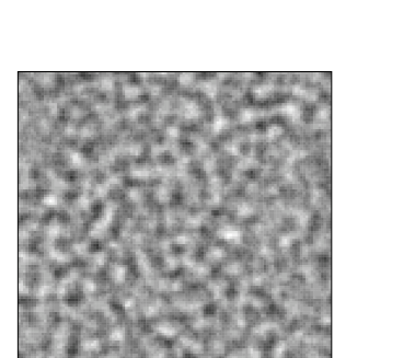
(b)         

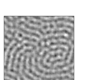
(c)         

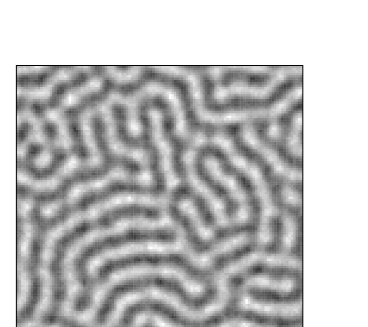
FIG. 3.: Patterns corresponding to the three situations named $A$, $B$ and $C$ in Fig. 1.

C Structure function in the convecting phase

In order to analyse more deeply the lack of finite-size effects in the convective heat flux above threshold, we have computed the stationary spherically-averaged structure function in a noise-favored convecting state (with a negative $r$ but a supercritical value of $D$). This function is defined as the Fourier transform of the correlation function of the system,

$$G\left(\vec{x},t\right)\;=\;\frac{1}{V}\,\int_{V}\,d\vec{x}\,^{\prime}\left<u\left(\vec{x}\,^{\prime},t\right)\,u\left(\vec{x}\,^{\prime}+\vec{x},t\right)\right>$$ (22)

Hence, the structure function indicates any periodicity in the system, so that it is a good way of characterising a pattern. Let us consider a finite system of volume $V$. The Fourier transform $u_{\mu}(t)$ of the field $u\left(\vec{x},t\right)$ is defined by:

$$u\left(\vec{x},t\right)\;=\;\frac{1}{V}\,\sum_{\mu}e^{i\vec{k}_{\mu}\cdot\vec{x}}\,u_{\mu}$$ (23)

where the components of $\vec{k}$ have the form $2\pi\mu/L$, where $\mu$ is an integer and $L$ is the corresponding linear dimension of the system. Then it can be seen that the structure function is:

$$S_{\mu}\;=\;\frac{1}{V}\,\left<u_{\mu}\,u_{-\mu}\right>$$ (24)

FIG. 4.: Structure function for the same convecting state with different system sizes.

Simulations show that this function behaves in the same way for the whole parameter range, presenting a unique maximum related to the periodicity of the pattern in the convecting phase and to thermal fluctuations in the conducting one, even though in this last case the height of the peak is several orders of magnitude lower than in the convecting one. Calculations have been performed for different system sizes in the patterned region, where the peaks are all seen to be centered at approximately the same value of $k$, $k\sim k_{0}$ (in this case $k_{0}\simeq 0.63$), but their heights increase and their widths decrease with increasing $L$ (see Fig. 4). In fact, it can be seen (Fig. 5) that $S_{max}\sim L$ and $\Delta S\sim L^{-1}$, so that the total area under the curve $S(k)$ is kept constant with varying $L$. This result agrees with the lack of finite-size effects in $J_{st}$, since the convective heat flux can be seen to be equal to the area under the structure function. All these facts lead to the conclusion that the structure function approaches a delta function in the thermodynamic limit (where the rolls are perfectly shaped) as the system size increases.

FIG. 5.: Logarithmic plots of the maximum and width of the structure function against system size. Linear fitting gives exponents $\sim+1$ and $\sim-1$, respectively.

III Linear stability analysis of the structure function

A linear stability analysis of the homogeneous $u=0$ solution of model (3) permits to estimate the transition point as that at which this solution becomes unstable. Beyond it the system departs from zero and becomes saturated by the nonlinearity, giving rise to the appearance of a non-zero roll solution. Due to the relevant role of the structure function as a means of characterising a patterned state, as has been discussed in the previous section, we shall begin our theoretical approach to the problem with a linear stability analysis of this function.

We now assume that the homogeneous conducting $u=0$ solution is affected by small perturbations, so that we only need to evaluate the evolution equation of $S_{\mu}$, defined in (24) in the linear regime. This can be done by using the Fokker-Planck equation governing the behaviour in time of the probability density of the field (in this case in Fourier space). As shown in the Appendix, the Fokker-Planck equation for the probability distribution of the stochastic process $u_{\mu}(t)$ is

$$\frac{\partial P}{\partial t}\;=\;-\sum_{\mu}\frac{\partial}{\partial u_{\mu}}F_{\mu}P\;+\;V\varepsilon\;\sum_{\mu,\nu}\;\frac{\partial}{\partial u_{\mu}}\;\frac{\partial}{\partial u_{-\mu}}\;P$$ (25)

$$+\;\frac{1}{V}\;\sum_{\mu,\nu,\nu^{\prime}}\;\frac{\partial}{\partial u_{\mu}}\;G_{\mu-\nu^{\prime}}\;D_{\nu^{\prime}}\;\frac{\partial}{\partial u_{\nu}}\;G_{\nu+\nu^{\prime}}\;P$$ (26)

where $D_{\nu}$ is the discrete Fourier transform of $D_{i-j}$, and $F$ and $G$ are the Fourier transforms of the corresponding terms in the discretized version of the SH equation (3):

$$\frac{du_{i}}{dt}\;=\;f_{i}\left(\vec{u}(t)\right)\;+\;\eta_{i}(t)\;+\;g_{i}\left(\vec{u}(t)\right)\;\xi_{i}(t)$$ (27)

So that

$$f_{i}=\left(r-\left(\nabla_{ij}^{2}+k_{0}^{2}\right)^{2}\right)u_{j}\;\;\;\;\;\;\;\;\;\;\;\;\;\;\;\;\;\;\;\;\;\;\;\;\;\;\;\;\;$$ (28)

$$\leftrightarrow\;F_{\mu}=\left(r-\left(\nabla_{\mu}^{2}+k_{0}^{2}\right)^{2}\right)u_{\mu}$$ (29)

$$g_{i}=u_{i}\leftrightarrow\;G_{\mu}=u_{\mu}\;\;\;\;\;\;\;\;\;\;\;\;\;\;\;\;\;\;\;\;\;\;\;\;\;\;\;\;\;$$ (30)

where $\nabla_{ij}$ and $\nabla_{\mu}$ are a discretized version of the Laplacian and its Fourier transform, respectively. The time evolution equation for $S_{\mu}$ is given by:

$$\frac{dS_{\mu}}{dt}=\frac{1}{V}\;\int{\cal D}u\;u_{\mu}u_{-\mu}\;\frac{\partial P}{\partial t}$$ (31)

When Fokker-Planck equation (26) is introduced in this expression and integration by parts is performed, the following equation is obtained:

$$V\;\frac{dS_{\mu}}{dt}=\left<u_{\mu}F_{-\mu}\right>+\left<u_{-\mu}F_{\mu}\right>\;\;\;\;\;\;\;\;\;\;\;\;\;\;\;\;\;$$ (32)

$$+\frac{1}{V}\int{\cal D}u\sum_{\eta,\nu,\nu^{\prime}}\delta_{\mu\eta}\;\delta_{-\mu\nu}\;G_{\eta-\nu^{\prime}}\;D_{\nu^{\prime}}\;G_{\nu+\nu^{\prime}}\;P$$ (33)

$$+\frac{1}{V}\int{\cal D}u\sum_{\eta,\nu,\nu^{\prime}}\delta_{\mu\eta}\;u_{-\mu}\;\frac{\partial G_{\eta-\nu^{\prime}}}{\partial u_{\nu}}\;D_{\nu^{\prime}}\;G_{\nu+\nu^{\prime}}\;P$$ (34)

$$+\frac{1}{V}\int{\cal D}u\sum_{\eta,\nu,\nu^{\prime}}\delta_{-\mu\eta}\;\delta_{\mu\nu}\;G_{\eta-\nu^{\prime}}\;D_{\nu^{\prime}}\;G_{\nu+\nu^{\prime}}\;P$$ (35)

$$+\frac{1}{V}\int{\cal D}u\sum_{\eta,\nu,\nu^{\prime}}\delta_{-\mu\eta}\;u_{\mu}\;\frac{\partial G_{\eta-\nu^{\prime}}}{\partial u_{\nu}}\;D_{\nu^{\prime}}\;G_{\nu+\nu^{\prime}}\;P\;$$ (36)

$$+\;2\,\varepsilon\;V$$ (37)

Introduction of (28) into this expression leads to

$$\frac{d}{dt}S_{\mu}(t)\;=\;2\left(r-\left(\nabla_{\mu}^{2}+k_{0}^{2}\right)^{2}\right)S_{\mu}(t)+2\varepsilon+$$ (38)

$$\frac{2}{V}\;S_{\mu}\;\sum_{\nu}D_{\nu}+\;\frac{2}{V^{2}}\;\sum_{\nu}D_{\nu}\left<u_{\mu-\nu}\,u_{-\mu+\nu}\right>$$ (39)

But, according to definition (23), the following relation holds:

$$\sum_{\nu}D_{\nu}=V\;D(\vec{x}=0)=V\;D(0)$$ (40)

Thus the equation for the structure function is finally

$$\frac{d}{dt}S_{\mu}(t)\;=\;2\left(r+D(0)-\left(\nabla_{\mu}^{2}+k_{0}^{2}\right)^{2}\right)S_{\mu}(t)$$ (41)

$$+2\varepsilon+2\;\frac{1}{V}\;\sum_{\nu}D_{\nu}S_{\mu-\nu}$$ (42)

Translation of this equation into its continuum version leads to the final expression for the evolution equation of the structure function of the Swift-Hohenberg model in the presence of a space-colored multiplicative external noise:

$$\frac{\partial}{\partial t}S(\vec{k},t)=2\left[r+D(0)-\left(k^{2}-k_{0}^{2}\right)^{2}\right]S(\vec{k},t)$$ (43)

$$+2\varepsilon+2\frac{1}{(2\pi)^{2}}\int D(\vec{q})S(\vec{k}-\vec{q},t)d\vec{q}$$ (44)

The stability analysis of this equation needs some comments. The last term in Eq. (43) is a mode-coupling term, which is essentially non-linear and will be discarded in our linear analysis. In this case, the presence of a multiplicative noise leads to the existence of an effective noise-dependent control parameter, $r+D(0)$, so that any perturbation of the homogeneous state will always grow if the condition $r+D(0)>0$ is obeyed. Hence, linear analysis predicts that, under the presence of multiplicative noise, the system can leave the homogeneous state in situations for which $r<0$. The nonlinearity will then stabilise the system in an ordered state. Besides, $D(0)=D/(4\lambda^{2})$ for the particular noise spectrum we have chosen, so that the amount of the shift decreases with increasing correlation length. This effect can be observed in the simulation results presented in Fig. 6, where a phase diagram of the system is plotted in the $(D,-r)$ plane for different values of the correlation length of the noise $\lambda$. It is worth noting that, as long as $D\neq 0$, the critical value of $r$ for the transition from conduction to convection is strictly negative. As predicted by our analysis, the critical curve in this plane is a straight line whose slope decreases as $\lambda$ increases, reducing the noise-favored region and thus the shift effect due to the multiplicative noise. In the figure, isolated symbols are transition points as obtained from simulations, whereas solid lines are the corresponding relations coming from the linear analysis ($r+D/(4\lambda^{2})=0$).

FIG. 6.: Phase diagram of the system in the ($D,-r$) plane for different values of the correlation length of the noise.

In the linear stability analysis of Ref. [16], the last term of Eq. (43) was considered and was proved to give corrections of order $D(0)^{2}$. On the other hand, the relevance of this term can be seen by studying the stationary structure function. From evolution equation (43), this function can be analytically found in the subcritical case ($r+\frac{D}{\Delta x^{2}}<0$) for a white external noise ($D(\vec{k})=D$), the result being:

$$S_{st}(k)\,=\,\frac{\varepsilon^{\prime}}{\left(k^{2}-k_{0}^{2}\right)^{2}+\mid r_{eff}\mid}\,=\,\frac{\varepsilon^{\prime}}{\omega(k)}$$ (45)

where the effective control parameter $r_{eff}$ is

$$r_{eff}\,=\,r+\frac{D}{\Delta x^{2}}$$ (46)

and the renormalised additive-noise intensity is

$$\varepsilon^{\prime}\,=\,\frac{\varepsilon}{1-\gamma D}$$ (47)

with

$$\gamma=-\frac{1}{4\pi}\,\mid r_{eff}\mid^{-1/2}\,arctg\mid r_{eff}\mid^{1/2}$$ (48)

$$=\frac{1}{(2\pi)^{2}}\,\int\frac{1}{\omega(k)}\,d\vec{k}$$ (49)

FIG. 7.: Simulation results for the spherically-averaged structure function for a conducting state with (circles) and without (diamonds) multiplicative noise. Dashed lines are the continuum analytical solutions coming from linear analysis, and the dotted line corresponds to the solution with no mode-coupling term ($\gamma$ set equal to $0$). Values of the parameters are $r=-0.2$, $\varepsilon=0.001$, $\Delta x=1.0$ and $k_{0}=0.63$.

FIG. 8.: Comparison of the spherically-averaged structure function obtained by simulation (diamonds), discrete integration of the analytical linear evolution equation (dashed line) and linear analytical continuum solution (solid line).

This linear result can be compared satisfactorily with (nonlinear) numerical simulations, since in the subcritical region nonlinear terms are expected to be negligible. Figure 8 shows both kind of results with and without multiplicative noise. The ordering role of this external noise is observed even in this conducting situation, enhancing the maximum value of the structure function at $k=k_{0}$. The growing discrepancy between theory and simulation at large wavenumbers can be understood from the fact that we are comparing an analytical result derived in a continuum space with numerical results coming from a discrete-space simulation. Figure 8 shows a comparison (for the case $D=0$) between these two results and a (discrete) numerical integration of Eq. (43). The agreement between these results and the simulation ones is quite good even at large wavenumbers.

It should be noted that making $\gamma=0$ in (45)-(49) amounts to ignoring the mode-coupling term in Eq. (43). Figure 8 shows that the result (45) with $\gamma=0$ is almost identical to the solution of the full linear analysis, in agreement with our previous statement concerning the lack of influence of the mode-coupling term in a first-order linear stability analysis.

IV Linear stability analysis of n-th order moments

Due to the stochastic character of the field $u\left(\vec{x},t\right)$, the linear stability analysis can also be done on the statistical moments of $u$. In this case, differences between the zero-dimensional and the spatially-extended cases appear, as will be discussed in what follows.

1 Zero-dimensional case

Let us consider the following zero-dimensional model, known as the Stratonovich model:

$$\frac{dx}{dt}\;=\;\alpha\,x-x^{3}+x\,\xi(t)$$ (50)

$$\left<\xi(t)\,\xi(t^{\prime})\right>=2\,D\,\delta(t-t^{\prime})$$ (51)

In the absence of noise, this model exhibits a supercritical pitchfork bifurcation at $\alpha=0$. For negative values of $\alpha$, the stable stationary solution of (50) is $x=0$. In the presence of the multiplicative noise, position of the bifurcation point can be given by a linear stability analysis of solution $x=0$. Since $x$ is now a stochastic process, the stability analysis is performed on its statistical moments, whose time evolution can be found from the Fokker-Planck equation governing the evolution of $P$. In the linear regime we have,

$$\frac{\partial P}{\partial t}\;=\;-\frac{\partial}{\partial x}\,\alpha x\,P\;+\;D\,\frac{\partial}{\partial x}\,x\,\frac{\partial}{\partial x}\,x\,P$$ (52)

where $P(x,t)$ is the probability density of the stochastic process $x(t)$. This equation leads to

$$\frac{d}{dt}\left<x^{n}\right>\;=\;n\,(\alpha+n\,D)\,\left<x^{n}\right>$$ (53)

which indicates that the bifurcation point for the n-th order moment is located at $\alpha_{c}=-n\,D$. Hence the position of the bifurcation point depends on the order of the statistical moment which is being analysed, which makes this analysis meaningless. We will see shortly that spatial coupling in extended systems introduces changes to this situation, leading to a useful analytical result.

2 Spatially-extended case

We now turn our attention back to the SH model with multiplicative noise (3). In order to obtain a possible higher-order generalisation of the structure function, let us consider the following correlation function:

$$G^{(n)}\left(\vec{x},t\right)\;=\;\frac{1}{V}\,\int_{V}\,d\vec{x}\,^{\prime}\left<\prod_{l=1}^{n}\,u\left(\vec{x}\,^{\prime}+(l-1)\vec{x},t\right)\right>$$ (54)

which measures the correlation between the values of the field at $n$ points equally spaced along a line. Its Fourier transform leads to a generalised n-th order structure function,

$$S^{(n)}_{\mu}\;=\;\frac{1}{V}\,\sum_{\mu_{1}}\,\sum_{\mu_{2}}\cdots\sum_{\mu_{n}}\,\left<\prod_{i=1}^{n}\,u_{\mu_{i}}\right>$$ (55)

$$\times\delta_{\sum_{i=1}^{n}\mu_{i},0}\,\delta_{\mu+\sum_{i=1}^{n}(i-1)\mu_{i},0}$$ (56)

Applying to this quantity the procedure described in the previous paragraphs, making use of the Fokker-Planck equation (26), performing integration by parts and ignoring internal noise, one finds

$$\frac{d}{dt}S^{(n)}_{\mu}(t)\;=\;n\left(r+D(0)-\left(\nabla_{\mu}^{2}+k_{0}^{2}\right)^{2}\right)S^{(n)}_{\mu}(t)$$ (57)

$$+\,\frac{n(n-1)}{V}\;\sum_{\nu}\,D_{\nu}\,S^{(n)}_{\mu-\nu}$$ (58)

Unlike the zero-dimensional case, all dependence on $n$ of the linear coefficient in the previous equation is factorised out. Hence, this results shows that spatial coupling prevents the linear analysis from giving different first-order results for different-order statistical moments (part of the contribution of the multiplicative noise comes through the inhomogeneous term in Eq. (58), which represents the coupling between spatial modes). There exist, of course, other possible methods to study and extract information from the behaviour of higher-order moments in pattern-forming systems (see, for instance [23]).

V Conclusion

Simulations of the Swift-Hohenberg model with a space-correlated fluctuating control parameter show that the bifurcation point from a homogeneous to a structured state is shifted from the standard additive-noise case. The amount of the shift increases with increasing intensity of the multiplicative noise, whereas space correlation in the fluctuations shifts back the transition point towards the standard situation. A good qualitative and quantitative agreement is obtained between this numerical study and a linear stability analysis of the structure function of the system, for the values of the parameters used here. The stability analysis has also been performed on a set of generalised structure functions which correspond to higher-order statistical moments, and the same results are found in all cases (i.e. for all orders) within our assumptions (i.e. at first order), which constitutes a qualitative difference to the role of multiplicative noise in zero-dimensional systems.

In conclusion, in this pattern-forming spatially extended system, multiplicative noise produces an unambiguous shift of the transition in the ordering direction. It is worth saying, however, that according to recent studies on other extended systems in the presence of multiplicative noise [17], one can expect that for large values of the intensity of this noise, the system will return to the disordered state.

Fokker-Planck equation for a spatially-extended process with multiplicative noise

In the following we shall assume a multiplicative noise with a non-delta correlation only in space:

$$\left<\;\xi(\vec{x},t)\;\xi(\vec{x}\,^{\prime},t^{\prime})\;\right>=2\;D(\vec{x}-\vec{x}\,^{\prime})\;\delta(t-t^{\prime})$$ (59)

Our aim now is to find the Fokker-Planck equation governing the stochastic process whose evolution is given by the general equation

$$\frac{\partial u\left(\vec{x},t\right)}{\partial t}=f\left(u\left(\vec{x},t\right),\nabla\right)+g\left(u\left(\vec{x},t\right),\nabla\right)\xi\left(\vec{x},t\right).$$ (60)

This can be easily done in Fourier space. In a first step the equation is written in a discrete space, where the Langevin equation is:

$$\frac{du_{i}}{dt}=f_{i}\left(u(t)\right)+g_{i}\left(u(t)\right)\xi_{i}(t)$$ (61)

where the cells have been named with one index independently of the dimension of the discrete space. The correlation of the noise in this discrete space is:

$$\left<\;\xi_{i}(t)\;\xi_{j}(t^{\prime})\;\right>=2\;D_{i-j}\;\delta(t-t^{\prime})$$ (62)

where $D_{i-j}$ is the discrete version of the continuous function $D$ describing the space decay of the correlation. In the limit of zero correlation length (white-noise limit) it becomes $\varepsilon\delta_{ij}/(\Delta x)^{d}$, where $\Delta x$ is the spacing of the lattice, i.e. the cell size.

Now we define the discrete Fourier transform and antitransform as

$$u_{\mu}=\left(\Delta x\right)^{d}\sum_{i}e^{-iq_{\mu}x_{i}}u_{i}$$ (63)

$$u_{i}=\frac{1}{(L\Delta x)^{d}}\sum_{\mu}e^{iq_{\mu}x_{i}}u_{\mu}$$ (64)

where $L$ is the number of cells per dimension, $q_{\mu}=\frac{2\pi}{L\Delta x}\mu$, $x_{i}=i\Delta x$ and the sums are d-fold going from 1 to L. It can be seen that the following relations hold:

$$\sum_{i}e^{i(q_{\mu}-q_{\mu^{\prime}})x_{i}}\;=\;L^{d}\;\delta_{\mu\mu^{\prime}}$$ (65)

$$\sum_{\mu}e^{iq_{\mu}(x_{i}-x_{j})}\;=\;L^{d}\;\delta_{ij}$$ (66)

The correlation of the noise in Fourier space, $\xi_{\mu}(t)$, can be seen to be

$$\left<\;\xi_{\mu}(t)\;\xi_{\nu}(t^{\prime})\;\right>=(L\Delta x)^{d}\;2\;D_{\mu}\;\delta_{-\mu,\nu}\;\delta(t-t^{\prime})$$ (67)

Here definitions (63) and properties (65) have been used.

The equation of evolution of $u_{\mu}$ comes from the Fourier transformation of Eq. (61):

$$\frac{du_{\mu}}{dt}=f_{\mu}+\left(\Delta x\right)^{d}\;\sum_{i}\;e^{-iq_{\mu}x_{i}}\;g_{i}\;\xi_{i}$$ (68)

The last term at the right-hand side can be evaluated in terms of the Fourier variables by means of (63) and (65):

$$\frac{du_{\mu}}{dt}=f_{\mu}+\frac{1}{(L\Delta x)^{d}}\;\sum_{\nu}\;g_{\mu-\nu}\;\xi_{\nu}$$ (69)

In the phase space of these Fourier variables we consider an ensemble of systems corresponding to a given realization of the noise and different initial conditions. The density of this ensemble $\rho\left(u,t\right)$ must verify a continuity Liouville equation:

$$\frac{\partial\rho}{\partial t}\;=\;-\sum_{\mu}\;\frac{\partial}{\partial u_{\mu}}\;\dot{u}_{\mu}\;\rho$$ (70)

where $\rho\left(u,t\right)=\left<\delta\left(u(t)-u\right)\right>_{IC}$, the average being taken over initial conditions only. On the other hand, the average of this density over the noise is the probability density of the stochastic process $P\left(u,t\right)=\left<\rho\right>$ (Van Kampen’s lemma [24]) whose evolution equation is the Fokker-Planck equation we are looking for. Performing this noise average on (70) leads thus to

$$\frac{\partial P}{\partial t}=-\sum_{\mu}\frac{\partial}{\partial u_{\mu}}f_{\mu}P-\frac{1}{(L\Delta x)^{d}}\;\sum_{\mu,\nu}\;\frac{\partial}{\partial u_{\mu}}\;g_{\mu-\nu}\;\left<\xi_{\nu}\rho\right>$$ (71)

The average in the last term of the second member of this equation can be evaluated by means of Novikov’s theorem [25], which states that for a gaussian stochastic process $\xi$ the following relation holds:

$$\left<\rho\left(u,t\right)\xi_{\nu}(t)\right>=\int_{0}^{t}dt^{\prime}\sum_{\eta}\left<\xi_{\nu}(t)\xi_{\eta}(t^{\prime})\right>\left<\frac{\partial\rho}{\partial\xi_{\eta}(t^{\prime})}\right>$$ (72)

and using (67) one finds

$$\left<\rho\left(u,t\right)\xi_{\nu}(t)\right>=\left(L\Delta x\right)^{d}D_{\nu}\left<\frac{\partial\rho}{\partial\xi_{-\nu}(t)}\right>$$ (73)

And this last average can be calculated in the following way:

$$\left<\frac{\partial\rho}{\partial\xi_{-\nu}(t)}\right>=\;\;\;\;\;\;\;\;\;\;\;\;\;\;\;\;\;\;\;\;\;\;\;\;\;\;\;\;\;\;\;\;\;\;\;\;\;\;\;\;\;\;\;\;\;\;\;\;\;\;$$ (74)

$$\sum_{\eta}\left<\frac{\delta u_{\eta}(t)}{\delta\xi_{-\nu}(t)}\;\frac{\partial}{\partial u_{\eta}(t)}\;\delta\left(u(t)-u\right)\right>$$ (75)

$$=-\sum_{\eta}\frac{\partial}{\partial u_{\eta}}\left<\left.\frac{\delta u_{\eta}(t)}{\delta\xi_{-\nu}(t)}\right|_{u(t)=u}\delta\left(u(t)-u\right)\right>$$ (76)

The functional derivative in this expression can be calculated from Eq. (69). The result is:

$$\frac{\delta u_{\eta}(t)}{\delta\xi_{-\nu}(t)}=\frac{1}{\left(L\Delta x\right)^{d}}\,g_{\eta+\nu}\left(u(t)\right)$$ (77)

so that the Fokker-Planck equation we are looking for is finally

$$\frac{\partial P}{\partial t}=-\sum_{\mu}\frac{\partial}{\partial u_{\mu}}f_{\mu}P\;\;\;\;\;\;\;\;\;\;\;\;\;\;\;\;\;\;\;\;\;\;\;\;\;\;\;\;\;\;\;\;\;\;\;\;\;\;\;\;$$ (78)

$$+\frac{1}{(L\Delta x)^{d}}\;\sum_{\mu,\nu,\eta}\;\frac{\partial}{\partial u_{\mu}}\;g_{\mu-\nu}\;D_{\nu}\;\frac{\partial}{\partial u_{\eta}}\;g_{\eta+\nu}\;P$$ (79)

In the particular case of a noise which is also white in space:

$$D_{i}=\varepsilon\frac{\delta_{i,0}}{(\Delta x)^{d}}\;\;\;\;\;\;\Longrightarrow\;\;\;\;\;\;D_{\mu}=\varepsilon$$ (80)

and the Fokker-Planck equation is

$$\frac{\partial P}{\partial t}=-\sum_{\mu}\frac{\partial}{\partial u_{\mu}}f_{\mu}P\;\;\;\;\;\;\;\;\;\;\;\;\;\;\;\;\;\;\;\;\;\;\;\;\;\;\;\;\;\;\;\;\;\;\;\;\;\;\;\;$$ (81)

$$+\frac{\varepsilon}{(L\Delta x)^{d}}\;\sum_{\mu,\nu,\eta}\;\frac{\partial}{\partial u_{\mu}}\;g_{\mu-\nu}\;\frac{\partial}{\partial u_{\eta}}\;g_{\eta+\nu}\;P$$ (82)

^∗ Permanent address: Dept. de Física i Enginyeria Nuclear, E.T.S. d’Enginyers Industrials de Terrassa, Univ. Politècnica de Catalunya, Colom 11, E-08222 Terrassa, Spain.

REFERENCES

- [1] M.C. Cross and P.C. Hohenberg, Rev. Mod. Phys. 65, 851 (1993).
- [2] P. Manneville, Dissipative Structures and Weak Turbulence (Academic Press, London, 1990).
- [3] S. Chandrasekhar, Hydrodynamic and hydromagnetic stability (Clarendon Press, Oxford, 1961).
- [4] C.W. Meyer, G. Ahlers and D.S. Cannell, Phys. Rev. Lett. 59, 1577 (1987).
- [5] M. Brambilla, M. Cattaneo, L.A. Lugiato, R. Pirovano, F. Prati, A.J. Kent, G.L. Oppo, A.B. Coates, C.O. Weiss, C. Green, E.J. D’Angelo and J.R. Tredicce, Phys. Rev. A 49, 1427 (1994).
- [6] J. Lega, P.K. Jakobsen, J.V. Moloney and A.C. Newell, Phys. Rev. A 49, 4201 (1994).
- [7] J. Swift and P.C. Hohenberg, Phys. Rev. A 15, 319 (1977).
- [8] H. Xi, J.D. Gunton and J. Viñals, Phys. Rev. E 47, R2987 (1993).
- [9] M.F. Hilali, S. Métens, P. Borckmans and G. Dewel, Phys. Rev. E 51, 2046 (1995).
- [10] P. Mandel, M. Georgiou and T. Erneux, Phys. Rev. A 47, 4277 (1993).
- [11] J. Lega, J.V. Moloney and A.C. Newell, Phys. Rev. Lett. 73, 2978 (1994); Physica D 83, 478 (1995).
- [12] W. Horsthemke and R. Lefever, Noise-Induced Transitions (Springer, Berlin, 1984).
- [13] C.R. Doering, H.R. Brand and R.E. Ecke, eds. External Noise and Its Interaction with Spatial Degrees of Freedom in Nonlinear Dissipative Systems, Workshop Proceedings, J. Stat. Phys. 54, 1111-1540 (1989).
- [14] K.R. Elder, J. Viñals and M. Grant, Phys. Rev. Lett. 68, 3024 (1992).
- [15] J. García-Ojalvo, A. Hernández-Machado and J.M. Sancho, Phys. Rev. Lett. 71, 1542 (1993).
- [16] A. Becker and L. Kramer, Phys. Rev. Lett. 73, 955 (1994); Physica D, in press.
- [17] C. Van den Broeck, J.M.R. Parrondo and R. Toral, Phys. Rev. Lett. 73, 3395 (1994).
- [18] J. García-Ojalvo, J.M. Sancho and L. Ramírez-Piscina, Phys. Lett. A 168, 35 (1992).
- [19] J. García-Ojalvo and J.M. Sancho, Phys. Rev. E 49, 2769 (1994).
- [20] J.M. Sancho, M. San Miguel, S. Katz and J.D. Gunton, Phys. Rev. A 26, 1589 (1982).
- [21] L. Ramírez-Piscina, J. M. Sancho and A. Hernández-Machado, Phys. Rev. B 48, 125 (1993).
- [22] J. García-Ojalvo, J.M. Sancho and L. Ramírez-Piscina, Phys. Rev. A 46, 4670 (1992).
- [23] A. Mikhailov, Physica A 188, 367 (1992).
- [24] N.G. Van Kampen, Phys. Rep. 24c, 171 (1976).
- [25] E.A. Novikov, Sov. Phys. JETP 20, 1290 (1965).