Renormalization of Drift and Diffusivity in Random Gradient Flows

Abstract

We investigate the relationship between the effective diffusivity and effective drift of a particle moving in a random medium. The velocity of the particle combines a white noise diffusion process with a local drift term that depends linearly on the gradient of a gaussian random field with homogeneous statistics. The theoretical analysis is confirmed by numerical simulation.

For the purely isotropic case the simulation, which measures the effective drift directly in a constant gradient background field, confirms the result previously obtained theoretically, that the effective diffusivity and effective drift are renormalized by the same factor from their local values. For this isotropic case we provide an intuitive explanation, based on a spatial average of local drift, for the renormalization of the effective drift parameter relative to its local value.

We also investigate situations in which the isotropy is broken by the tensorial relationship of the local drift to the gradient of the random field. We find that the numerical simulation confirms a relatively simple renormalization group calculation for the effective diffusivity and drift tensors.

DAMTP-96-34

1 Introduction

A problem of great interest concerns the computation of effective parameters for a diffusion process that combines molecular diffusion with a drift term linearly dependent on the gradient of a random scalar field with spatially homogeneous statistics. In the case where the system, including the statistical properties of the random field, is isotropic it has been shown, on the basis of plausible but not completely established assumptions, that the effective long range diffusivity is accurately predicted by a renormalization group calculation (RGC) [1, 2, 3]. The result, which is embodied in a very simple formula, is confirmed by numerical simulation to high accuracy. The result is also consistent with the straightforward perturbation expansion to two-loop order but remains accurate beyond the applicability of the expansion to this order [2, 4].

An important parameter relevant to the long time behaviour of the system, that has not generally been studied, is the value of the effective drift parameter, or tensor, that determines the average drift of particles in an imposed large-scale field gradient. A feature of the isotropic case, respected by the RGC, is that this effective drift coefficient is renormalized relative to its local value by the same factor as the effective diffusivity is renormalized relative to the molecular diffusivity [1, 2, 3, 4]. By including an appropriate constant drift term in the original molecular diffusion process we confirm, in this paper, directly by numerical simulation, the equality of the two renormalization factors. We also give an intuitive explanation in terms of spatial averages, of why one should expect that the drift coefficient be renormalized.

Isotropy can break down for three reasons. First, the statistics of the random field may not be isotropic. We have investigated this in a previous paper [5] and shown that, although the predictions of the RGC are still reasonably accurate there are emerging disparities with the results of the numerical simulation. Such an outcome is to be expected since the results of the RGC were, in this case, shown to differ from straightforward perturbation theory at two-loop order. Second, the molecular diffusion tensor may be non-isotropic and third, the same may be true of the local drift tensor. It is this third possibility that we investigate in this paper by numerical simulation and compare with the predictions of the appropriate RGC. The results actually agree rather well suggesting that the isotropy of the random field statistics is an important condition for the success of the RGC.

2 Diffusion with Background Drift

It is convenient for the purpose of discussing anisotropy to consider the most general diffusion equation of the class in which we are interested. It has the form

$$\frac{\partial~{}P}{\partial~{}t}=\partial_{i}(\kappa^{0}_{ij}\partial_{j}-\lambda^{0}_{ij}\partial_{j}\phi({\bf x})-u_{i})P~{}~{}.$$ (1)

Here $P$ is the probability density of a particle moving according to the equation

$$\dot{x}_{i}=\lambda^{0}_{ij}\partial_{j}\phi({\bf x})+u_{i}+w_{i}(t)~{}~{},$$ (2)

where the white noise term has zero mean and the correlation function

$$\langle w_{i}(t)w_{j}(t^{\prime})\rangle=2\kappa^{0}_{ij}\delta(t-t^{\prime})~{}~{},$$ (3)

and $u_{i}$ is a constant drift term. In appropriate units we would expect the drift to be given by

$$u_{i}=\lambda^{0}_{ij}g_{j}~{}~{},$$ (4)

where $g_{i}$ is a uniform gradient field.

The equation for the static Green’s function corresponding to a unit source at ${\bf x}^{\prime}$ is

$$\partial_{i}\left(\kappa^{0}_{ij}\partial_{j}-\lambda^{0}_{ij}\partial_{j}\phi({\bf x})-u_{i}\right)G({\bf x},{\bf x}^{\prime})=-\delta({\bf x}-{\bf x}^{\prime})~{}~{}.$$ (5)

The effective Green’s function obtained after averaging over the random ensemble of flows we denote by ${\cal G}({\bf x}-{\bf x}^{\prime})$ . It is simpler to study this function in terms of its Fourier transform. It has the form

$$\tilde{{\cal G}}({\bf k})=[\kappa^{0}_{mn}k_{m}k_{n}-\SS({\bf k})+iu_{j}W_{j}({\bf k})]^{-1}~{}~{}.$$ (6)

At small ${\bf k}$ the irreducible two-point function $\SS({\bf k})$ satifies

$$\SS({\bf k})\sim\sigma_{ij}k_{i}k_{j}~{}~{},$$ (7)

with the result that the effective long range diffusivity is

$$\kappa_{ij}=\kappa^{0}_{ij}-\sigma_{ij}~{}~{},$$ (8)

and

$$W_{j}({\bf k})\sim k_{i}\mu_{ij}.$$ (9)

for some coefficient $\mu_{ij}$ that we now evaluate. We show below that

$$W_{i}=[(\lambda^{0})^{-1}]_{im}V_{m}(0,{\bf k})~{}~{},$$ (10)

where $V_{m}({\bf q},{\bf k})$ is the (Fourier transform of the) vertex function that measures the influence of a weak external field on ${\cal G}({\bf x},{\bf x}^{\prime})$ . It is calculated below. For small ${\bf k}$ we have

$$V_{m}(0,{\bf k})\sim k_{n}\lambda_{nm}~{}~{},$$ (11)

where $\lambda_{mn}$ is the effective coupling referred to in the introduction. It follows that for small ${\bf k}$

$$\tilde{{\cal G}}({\bf k})\sim[\kappa_{mn}k_{m}k_{n}+ik_{m}\lambda_{mn}g_{n}]^{-1}~{}~{}.$$ (12)

The interpretation of this result is that the effective drift is

$$u^{\mbox{e}}_{m}=\lambda_{mn}g_{n}~{}~{}.$$ (13)

The measurement of the effective drift in a given external field allows us to extract the effective coupling $\lambda_{ij}$ from the simulation.

For the purposes of simulation we assumed that

$$\Delta({\bf x}-{\bf x}^{\prime})=\int\frac{d^{3}{\bf q}}{(2\pi)^{3}}D({\bf q})e^{i{\bf q}.({\bf x}-{\bf x}^{\prime})}~{}~{},$$ (14)

with

$$D({\bf q})=\frac{(2\pi)^{3\over 2}}{k_{0}^{3}}e^{-q^{2}/2k_{0}^{2}}~{}~{}.$$ (15)

With this normalization

$$\langle(\phi({\bf x}))^{2}\rangle=\Delta(0)=1~{}~{}.$$ (16)

3 Graphical Rules for Perturbation Theory

The Feynman rules for the diagrammatic perturbation expansion are essentially tha same as in the isotropic case. We have

• The sum of the inwardly flowing wave-vectors at each vertex is zero.

• Each solid line carries a factor of $\displaystyle{{1\over{\kappa^{0}_{ij}k_{i}k_{j}}}}$.

• Each loop wave-vector ${\bf q}$ is integrated with a factor $\displaystyle{{d^{3}{\bf q}\over(2\pi)^{3}}}$.

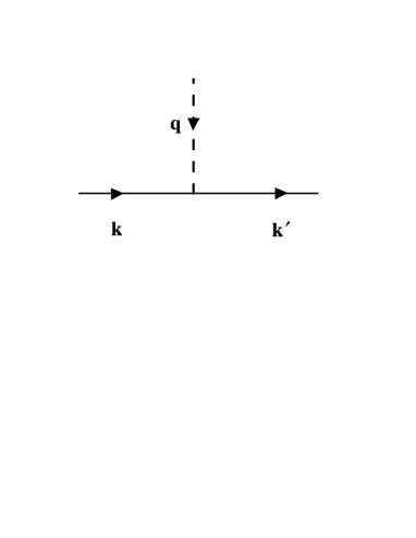
Figure 1: Vertex diagram

• Each vertex of the form of Fig. 1 carries a factor $q_{i}\lambda^{0}_{ij}\left({\bf k}+{\bf q}\right)_{j}$.

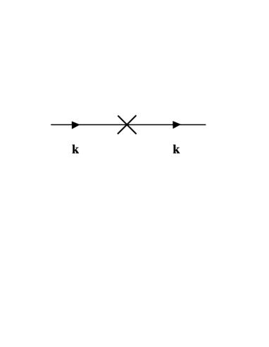
Figure 2: Drift insertion vertex

• Each vertex of the form of Fig. 2 carries a factor $-iu_{j}k_{j}$.

• Each dashed line carries a factor $D\left({\bf q}\right)$.

4 One-Loop Contributions

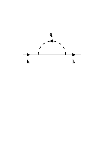
Figure 3: One–loop contribution to $\Sigma$

The one-loop contribution to $\SS({\bf k})$ is associated with Fig. 3 . It is, according to the Feynman rules,

$$\SS^{(1)}({\bf k})=-\int\frac{d^{3}{\bf q}}{(2\pi)^{3}}D({\bf q})\frac{({\bf k}+{\bf q})_{i}\lambda^{0}_{ij}q_{j}~{}k_{m}\lambda^{0}_{mn}q_{n}}{({\bf k}+{\bf q})_{r}\kappa^{0}_{rs}({\bf k}+{\bf q})_{s}}~{}~{}.$$ (17)

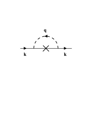
Figure 4: One-loop correction to drift insertion

The one-loop contribution to $u_{i}W_{i}({\bf k})$ is associated with Fig. 4 . The Feynman rules imply that it has the form

$$u_{i}W_{i}({\bf k})=-\int\frac{d^{3}{\bf q}}{(2\pi)^{3}}\frac{({\bf k}+{\bf q})_{i}\lambda^{0}_{ij}q_{j}~{}(-iu_{j}({\bf k}+{\bf q})_{j})~{}k_{m}\lambda^{0}_{mn}q_{n}}{(({\bf k}+{\bf q})_{r}\kappa^{0}_{rs}({\bf k}+{\bf q})_{s})^{2}}~{}~{}.$$ (18)

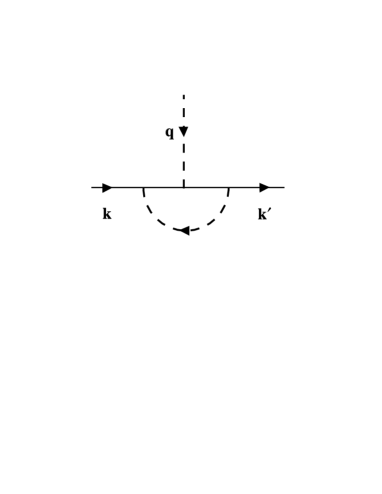
Figure 5: One loop correction to vertex

If we compare this result with that for the general vertex at one-loop associated with Fig. 5, namely

$$V_{i}({\bf q},{\bf k}^{\prime})=-\int\frac{d^{3}{\bf q}}{(2\pi)^{3}}\frac{({\bf k}+{\bf q})_{j}\lambda^{0}_{jl}q_{l}~{}\lambda^{0}_{ip}({\bf k}^{\prime}+{\bf q})_{p}~{}k^{\prime}_{m}\lambda^{0}_{mn}q_{n}}{({\bf k}+{\bf q})_{r}\kappa^{0}_{rs}({\bf k}+{\bf q})_{s}({\bf k}^{\prime}+{\bf q})_{u}\kappa^{0}_{uv}({\bf k}^{\prime}+{\bf q})_{v}}~{}~{}.$$ (19)

we see immediately that

$$V_{i}(0,{\bf k})=\lambda^{0}_{ij}W_{j}({\bf k})~{}~{}.$$ (20)

This result is easily generalized to all orders in perturbation theory. It is equivalent to the relation used in a previous paper [4].

5 Spatial Averages and Mean Drift

Some insight into the renormalization of the drift coefficient in the isotropic case ($\lambda^{(0)}_{ij}=\lambda_{0}\delta_{ij}$ and $\kappa^{(0)}_{ij}=\kappa_{0}\delta_{ij}$) can be obtained by considering a situation in which we allow a large cloud of particles to equilibriate in a large cubical sample with periodic boundary conditions. We then disturb the situation by imposing a uniform background drift field ${\bf g}$ causing a mean drift in the particle cloud. The average velocity of the particles is then renormalized relative to the mean local drift because of the lack of uniformity in the background probability distribution adopted by the particles.

In the absence of a background drift field the particles adopt a density distribution $P_{0}({\bf x})$ that yields zero particle current. That is

$${\bf J}=(\kappa_{0}\nabla-\lambda_{0}\nabla\phi({\bf x}))P_{0}({\bf x})=0~{}~{}.$$ (21)

The solution of this equation is

$$P_{0}({\bf x})=N\exp\{\frac{\lambda_{0}}{\kappa_{0}}\phi({\bf x})\}~{}~{},$$ (22)

where we will choose $N$ so that $P_{0}({\bf x})$ can be viewed as a probability distribution.

$$\int_{\mbox{cube}}d^{3}{\bf x}P_{0}({\bf x})=1~{}~{}.$$ (23)

For a very large cube it is acceptable to enforce this equation as an ensemble average. This allows us to evaluate $N$ as

$$N=\left(V\exp\left\{\frac{1}{2}\left(\frac{\lambda_{0}}{\kappa_{0}}\right)^{2}\Delta(0)\right\}\right)^{-1}~{}~{},$$ (24)

where $V$ is the volume of the cube.

When an external constant drift ${\bf g}$ is applied the system equilibriates with a new distribution $P_{0}+P_{1}$ that satisfies

$$\nabla.(\kappa_{0}\nabla-\lambda_{0}\nabla\phi({\bf x})-\lambda_{0}{\bf g})(P_{0}({\bf x})+P_{1}({\bf x}))=0~{}~{}.$$ (25)

It turns out that no change of normalization is required. This leads to the solution, correct to $O({\bf g})$, for $P_{1}$

$$P_{1}({\bf x})=-\lambda_{0}\int d^{3}{\bf x}^{\prime}G({\bf x},{\bf x}^{\prime})\nabla P_{0}({\bf x}^{\prime}).{\bf g}~{}~{}.$$ (26)

where $G({\bf x},{\bf x}^{\prime})$ is the Green’s function for the problem without drift.

At a point ${\bf x}$ in a given sample of the medium the velocity of a particle is $\lambda_{0}(\nabla\phi({\bf x})+{\bf g})$ after averaging over molecular diffusion effects. The the drift ${\bf u}$ of particles in the steady state situation with drift can be obtained as a spatial average of this velocity over the large cubical sample.

$${\bf u}=\lambda_{0}\int d^{3}{\bf x}(\nabla\phi({\bf x})+{\bf g})(P_{0}({\bf x})+P_{1}({\bf x}))$$ (27)

To $O({\bf g})$ we have

$$u_{i}=\lambda_{0}[\delta_{ij}-\lambda_{0}\int d^{3}{\bf x}d^{3}{\bf x}^{\prime}(\partial_{i}\phi({\bf x}))G({\bf x},{\bf x}^{\prime})\partial_{j}P_{0}({\bf x}^{\prime})]g_{j}~{}~{}.$$ (28)

In fact it is reasonable now to take the ensemble average of this quantity, with the result

$$u_{i}=\lambda_{0}[\delta_{ij}-\lambda_{0}\int d^{3}{\bf x}d^{3}{\bf x}^{\prime}\langle(\partial_{i}\phi({\bf x}))G({\bf x},{\bf x}^{\prime})\partial_{j}P_{0}({\bf x}^{\prime})\rangle]g_{j}~{}~{}.$$ (29)

To lowest (non-trivial) order in $\lambda_{0}$ we can replace $G({\bf x},{\bf x}^{\prime})$ by $G_{0}({\bf x}-{\bf x}^{\prime})$ and use the identity

$$\langle\phi({\bf x})P_{0}({\bf x}^{\prime})\rangle=\frac{\lambda_{0}}{\kappa_{0}}\Delta({\bf x}-{\bf x}^{\prime})/V~{}~{},$$ (30)

to obtain

$$u_{i}=\lambda_{0}[\delta_{ij}-\frac{\lambda_{0}^{2}}{\kappa_{0}}\int d^{3}{\bf x}G_{0}({\bf x})\partial_{i}\partial_{j}^{\prime}\Delta({\bf x})]g_{j}~{}~{}.$$ (31)

Expressing this in Fourier space we have

$$u_{i}=\lambda_{0}[\delta_{ij}-\frac{\lambda_{0}^{2}}{\kappa_{0}^{2}}\int\frac{d^{3}{\bf q}}{(2\pi)^{3}}D(q)\frac{q_{i}q_{j}}{q^{2}}]g_{j}~{}~{}.$$ (32)

Taking into account the isotropy of the statistical ensemble that we assume in this case, we see that ${\bf u}=\lambda_{\mbox{e}}{\bf g}$ where

$$\lambda_{\mbox{e}}=\lambda_{0}\left(1-\frac{1}{3}\frac{\lambda_{0}^{2}}{\kappa_{0}^{2}}\Delta(0)\right)$$ (33)

This is identical with the one-loop perturbation result of previous work [1, 2, 3, 4]. A careful analysis of the two-loop diagrams confirms the result to this order. This of course, is consistent with the RGC result

$$\lambda_{\mbox{e}}=\lambda_{0}\exp\left\{-\frac{1}{3}\frac{\lambda_{0}^{2}}{\kappa_{0}^{2}}\Delta(0)\right\}~{}~{},$$ (34)

discovered previously. From this point of view then the origin of the renormalization of the effective drift term comes about because in a steady state the particles adopt, in a given sample, a non-uniform distribution, appropriate to the sample, and the resulting spatial average of the local drift is modified relative to the local ensemble average which yields the local mean value. This should be contrasted with the situation in incompressible flow where the steady state distribution of particles inevitably remains uniform leading to a spatial average that coincides with the ensemble average and no renormalization of the drift coefficient.

6 Simulation of Drift in the Isotropic Case

In Table 1 we exhibit the results of measuring both $\kappa_{\mbox{e}}$ and $\lambda_{\mbox{e}}$, for an isotropic situation, over a range of values of the disorder parameter $\lambda_{0}/\kappa_{0}$ . We assume $\kappa_{0}=1$ and $k_{0}=1$ throughout. The simulation,

$N$	$\lambda_{0}$	$g$	$\kappa_{\mbox{e}}$	$(\lambda_{\mbox{e}}/\lambda_{0})$
128	1.0	.05	.722(2)	.726(2)
			(.717)	(.717)
256	1.5	.05	.470(5)	.474(2)
			(.472)	(.472)
256	2.0	.05	.269(4)	.266(11)
			(.264)	(.264)
512	2.5	.05	.139(5)	.140(20)
			(.125)	(.125)

Table 1: $N$ is the number of modes in random field. Theoretical values in brackets.

which is based on a continuum construction for $\phi({\bf x})$, has been described in previous papers [3, 4, 5]. An important point for the present paper is that the random field is constructed from a set of $N$ modes and the integrity of the Gaussian property of the statistics of the random field is dependent on having a sufficiently large value of $N$ .

The results clearly show the equality of the two renormalization parameters for a wide range of disorder parameter. This common value is also equal, as was found in previous work, to the RGC prediction of $\exp{\{-{1\over 3}{\lambda_{0}^{2}/\kappa_{0}^{2}}\}}$. There is a slight discrepancy at the higher values of the disorder parameter. We feel that this is a systematic error in the simulation due to the limited number of modes incorporated in the random field. Another possible source of error is that the value of the drift parameter has become so large that $O(g^{2})$ effects are influencing the values of the measured quantities. It is also possible that the assumptions behind the renormalization group calculation may no longer be valid at these values of $\lambda_{0}$ . It is interesting to note that, nevertheless the equality of the two renormalization factors is maintained throughout with particular accuracy. We can be reasonably confident therefore of our renormalization group results and the associated Ward identity [4, 5] in this isotropic case.

7 “Ward” Identity

In previous work we suggested a Ward identity as an explanation of the proportionality of the renormalization of the vertex and diffusivity matrix. The identity was verified to two-loop order in perturbation theory. Here we show that this Ward identity changes form when the bare vertex and diffusivity matrices are no longer proportional to one another. We will only discuss the the change at one-loop order since this is sufficient to demonstrate the breakdown.

From the formulae of the previous section we see that to one-loop

$$\frac{\partial}{\partial k_{i}}\SS({\bf k})=[\kappa^{0}(\lambda^{0})^{-1}]_{ij}V_{j}({\bf k},{\bf k})+U_{i}({\bf k})~{}~{},$$ (35)

where

$$U_{i}({\bf k})=-\int\frac{d^{3}{\bf q}}{(2\pi)^{3}}D({\bf q})\frac{q_{r}\lambda^{0}_{ri}q_{m}\lambda^{0}_{mn}k_{n}+q_{r}\lambda^{0}_{rs}({\bf q}+{\bf k})_{s}q_{m}\lambda^{0}_{mi}}{({\bf q}+{\bf k})_{j}\kappa^{0}_{jl}({\bf q}+{\bf k})_{l}}~{}~{}.$$ (36)

For small ${\bf k}$ we see that

$$k_{i}U_{i}({\bf k})=-\int\frac{d^{3}{\bf q}}{(2\pi)^{3}}D({\bf q})\left\{\frac{2(q_{s}\lambda^{0}_{rs}k_{s})^{2}}{q_{m}\kappa^{0}_{mn}q_{n}}-\frac{2q_{r}\lambda^{0}_{rs}q_{s}~{}q_{n}\lambda^{0}_{mn}k_{n}~{}q_{j}\kappa^{0}_{jl}k_{l}}{(q_{m}\kappa^{0}_{mn}q_{n})^{2}}\right\}+O(k^{4})~{}~{}.$$ (37)

It is easy to see that that the right side of this equation vanishes to $O(k^{4})$ when $\kappa^{0}\propto\lambda^{0}$ . In general however it does not do so. A simple case to consider is one in which the statistics of the $\phi({\bf x})$-field are isotropic, the diffusivity has the form $\kappa^{0}_{ij}=\kappa_{0}\delta_{ij}$ but the drift coefficient retains an anisotropic tensorial structure. We easily evaluate the right side of eq(37) to be

$$k_{i}U_{i}({\bf k})=-\frac{2\Delta(0)}{3\kappa_{0}}\left\{\frac{3}{5}k_{i}[(\lambda^{0})^{2}]_{ij}k_{j}-\frac{1}{5}\lambda^{0}_{mm}k_{i}\lambda^{0}_{ij}k_{j}\right\}+O(k^{4})~{}~{}.$$ (38)

If we define

$$\bar{\lambda}^{0}_{ij}=\lambda^{0}_{ij}-\frac{1}{3}\lambda^{0}_{mm}~{}~{},$$ (39)

so that $\bar{\lambda}^{0}$ is the traceless or quadrupole part of $\lambda^{0}$ then we can recast the above equation in the form

$$k_{i}U_{i}({\bf k})=-\frac{2\Delta(0)}{3\kappa_{0}}\left\{\frac{3}{5}k_{i}[(\bar{\lambda}^{0})^{2}]_{ij}k_{j}+\frac{1}{5}\lambda^{0}_{mm}k_{i}\bar{\lambda}^{0}_{ij}k_{j}\right\}+O(k^{4})~{}~{},$$ (40)

that is

$$k_{i}U_{i}({\bf k})=-\frac{2\Delta(0)}{5\kappa_{0}}k_{i}[\bar{\lambda}^{0}\lambda^{0}]_{ij}k_{j}+O(k^{4})~{}~{}.$$ (41)

This form of the result makes it clear that when the traceless part of the drift tensor $\bar{\lambda}^{0}$ vanishes we return to the situation in which the original Ward identity holds.

For the particular case we are considering the the modified Ward identity implies for small ${\bf k}$ the result

$$\frac{\partial}{\partial k_{i}}\SS({\bf k})=-\frac{\Delta(0)}{15\kappa_{0}}\left\{\lambda^{0}_{mm}\lambda^{0}_{ij}+2\lambda^{0}_{il}\lambda^{0}_{lj}\right\}k_{j}-\frac{2\Delta(0)}{3\kappa_{0}}\left\{\frac{3}{5}[(\lambda^{0})^{2}]_{ij}k_{j}-\frac{1}{5}\lambda^{0}_{mm}\lambda^{0}_{ij}k_{j}\right\}+O(k^{3})~{}~{}.$$ (42)

On the basis of this calculation we do not expect a simple relationship between the macroscopic diffusivity and the macroscopic drift coefficient. This is confirmed in the next section by a renormalization group calculation.

8 Renormalization Group Equations

The breakdown of the Ward identity and the absence of any simple relation between the effective diffusivity and drift tensors makes it interesting to examine the consequences of the renormalization group approach to computing the macroscopic parameters. These equations for the diffusivity tensor were written down in refs [4, 5]. We complete the scheme here with the corresponding equation for the drift coefficient. For simplicity we write down the equations for the wavenumber slicing scheme. They are

$$\frac{d\kappa_{ij}}{d\Lambda}=\int\frac{d^{3}{\bf q}}{(2\pi)^{3}}\delta(q-\Lambda)D(q)\frac{(q_{m}\kappa_{mi}q_{n}\lambda_{nj}+q_{m}\kappa_{mj}q_{n}\lambda_{ni})q_{r}\lambda_{rs}q_{s}-q_{m}\lambda_{mi}q_{n}\lambda_{nj}q_{r}\kappa_{rs}q_{s}}{(q_{r}\kappa_{rs}q_{s})^{2}}$$ (43)

and

$$\frac{d\lambda_{ij}}{d\Lambda}=\int\frac{d^{3}{\bf q}}{(2\pi)^{3}}\delta(q-\Lambda)D(q)\frac{q_{m}\lambda_{mi}q_{n}\lambda_{nj}q_{r}\lambda_{rs}q_{s}}{(q_{r}\kappa_{rs}q_{s})^{2}}$$ (44)

It is clear from these equations that, as mentioned in a previous paper [5], those solutions satisfying boundary conditions for which $\lambda^{0}_{ij}\propto\kappa^{0}_{ij}$ maintain the the proportionality $\lambda_{ij}(\Lambda)\propto\kappa_{ij}(\Lambda)$ for all $\Lambda$ with a constant ratio.

It is easily checked that of course the isotropic solutions are those of earlier papers, namely

$$\kappa_{ij}(\Lambda)=\kappa^{S}_{ij}(\Lambda)=\kappa_{0}\exp\left\{-\frac{1}{3}\frac{\lambda^{2}_{0}}{\kappa^{2}_{0}}\Delta_{\Lambda}(0)\right\}\delta_{ij}$$ (45)

and

$$\lambda_{ij}(\Lambda)=\lambda^{S}_{ij}(\Lambda)=\lambda_{0}\exp\left\{-\frac{1}{3}\frac{\lambda^{2}_{0}}{\kappa^{2}_{0}}\Delta_{\Lambda}(0)\right\}\delta_{ij}$$ (46)

where

$$\Delta_{\Lambda}(0)=\int_{q>\Lambda}\frac{d^{3}{\bf q}}{(2\pi)^{3}}D(q)~{}~{}.$$ (47)

We can examine solutions nearby these isotropic solutions, that are perturbed by a small anisotropic change in the local drift tensor. It is no restriction to make this small change traceless. We have then

$$\kappa_{ij}(\Lambda) = \kappa^{S}_{ij}(\Lambda)+\eta_{ij}$$ (48)

$$\lambda_{ij}(\Lambda) = \lambda^{S}_{ij}(\Lambda)+\mu_{ij}$$

where

$$\eta_{ij}(\infty) = 0$$ (49)

$$\mu_{ij}(\infty) = \mu^{0}_{ij}$$

with $\mu^{0}_{ii}=0$ . A perturbative analysis of eqs(43,44) yields

$$\frac{d\eta_{ij}}{d\Lambda} = \frac{\lambda_{0}}{\kappa_{0}}\int\frac{d^{3}{\bf q}}{(2\pi)^{3}}\delta(q-\Lambda)D(q)\left\{\frac{\lambda_{0}}{\kappa_{0}}\frac{2}{3}\eta_{ij}-\frac{3}{15}\frac{\lambda_{0}}{\kappa_{0}}(\eta\delta_{ij}+2\eta_{ij})\right.$$

$$~{}~{}~{}~{}~{}~{}~{}~{}~{}~{}~{}~{}~{}~{}~{}~{}~{}~{}~{}~{}~{}~{}~{}~{}~{}~{}~{}~{}~{}~{}~{}~{}~{}~{}~{}~{}~{}~{}~{}~{}~{}~{}~{}~{}~{}~{}~{}~{}~{}~{}~{}~{}~{}~{}~{}~{}\left.+\frac{2}{15}(\mu\delta_{ij}+2\mu_{ij})\right\}$$

$$\frac{d\mu_{ij}}{d\Lambda} = \frac{\lambda_{0}^{2}}{\kappa_{0}^{2}}\int\frac{d^{3}{\bf q}}{(2\pi)^{3}}\delta(q-\Lambda)D(q)\left\{\frac{2}{3}\mu_{ij}+\frac{1}{15}(\mu\delta_{ij}+2\mu_{ij})-\frac{2}{15}\frac{\lambda_{0}}{\kappa_{0}}(\eta\delta_{ij}+2\eta_{ij})\right\}$$

If we introduce a variable $0<s<1$ such that

$$s=\int_{q<\Lambda}\frac{d^{3}{\bf q}}{(2\pi)^{3}}D(q)$$ (51)

and impose the allowed constraint that $\eta=\eta_{ii}=0$ and $\mu=\mu_{ii}=0$ we find

$$\frac{d\eta_{ij}}{d~{}s} = \frac{4}{15}\frac{\lambda_{0}^{2}}{\kappa_{0}^{2}}\eta_{ij}+\frac{4}{15}\frac{\lambda_{0}}{\kappa_{0}}\mu_{ij}$$ (52)

$$\frac{d\mu_{ij}}{d~{}s} = \frac{12}{15}\frac{\lambda_{0}^{2}}{\kappa_{0}^{2}}\mu_{ij}-\frac{4}{15}\frac{\lambda_{0}^{3}}{\kappa_{0}^{3}}\eta_{ij}$$

These equations are easily integrated and yield the result

$$\kappa_{ij} = \kappa_{0}\exp\left\{-\frac{1}{3}\frac{\lambda_{0}^{2}}{\kappa_{0}^{2}}\right\}\delta_{ij}-\frac{4}{15}\frac{\lambda_{0}}{\kappa_{0}}\exp\left\{-\frac{8}{15}\frac{\lambda_{0}^{2}}{\kappa_{0}^{2}}\right\}\mu^{0}_{ij}$$ (53)

$$\lambda_{ij} = \lambda_{0}\exp\left\{-\frac{1}{3}\frac{\lambda_{0}^{2}}{\kappa_{0}^{2}}\right\}\delta_{ij}+\left(1-\frac{4}{15}\frac{\lambda_{0}^{2}}{\kappa_{0}^{2}}\right)\exp\left\{-\frac{8}{15}\frac{\lambda_{0}^{2}}{\kappa_{0}^{2}}\right\}\mu^{0}_{ij}$$

It follows that

$$(\lambda\kappa^{-1})_{ij}=\frac{\lambda_{0}}{\kappa_{0}}\left(\delta_{ij}+\frac{1}{\lambda_{0}}\exp\left\{-\frac{1}{5}\frac{\lambda_{0}^{2}}{\kappa_{0}^{2}}\right\}\mu^{0}_{ij}\right)~{}~{}.$$ (54)

For this near isotropic case at least we see that the proportionality of the macroscopic drift and diffusivity tensors is restored exponentially as the renormalization process takes place.

9 Numerical Simulation in the Anisotropic Case

We tested the above results from the renormalization group calculation against a simulation for which the asymmetric local drift tensor is diagonal in the coordinate basis with elements

$$\mu^{0}=\left(\begin{array}[]{ccc}-\alpha/2&0&0\\ 0&-\alpha/2&0\\ 0&0&\alpha\end{array}\right)~{}~{}.$$ (55)

Because of the axial symmetry of the local drift tensor the same property ensures that the effective diffusion and drift tensors will have the form

$$\kappa_{\mbox{e}}=\left(\begin{array}[]{ccc}\kappa_{\perp}&0&0\\ 0&\kappa_{\perp}&0\\ 0&0&\kappa_{\parallel}\end{array}\right)~{}~{}~{}~{}\mbox{and}~{}~{}~{}~{}\lambda_{\mbox{e}}=\left(\begin{array}[]{ccc}\lambda_{\perp}&0&0\\ 0&\lambda_{\perp}&0\\ 0&0&\lambda_{\parallel}\end{array}\right)$$ (56)

The results of the numerical simulation for certain values of $\lambda_{0}$ and various values of $\alpha$ are shown in Table 2.

$\lambda_{0}$	$\alpha$	$\kappa_{\parallel}$	$\kappa_{\perp}$	$\lambda_{\parallel}$	$\lambda_{\perp}$
1.	.2	.701(3)	.735(3)	.798(5)	.660(5)
		(.685)	(.732)	(.803)	(.674)
1.	.1	.698(3)	.727(2)	.770(6)	.687(5)
		(.701)	(.724)	(.760)	(.695)
1.	-.1	.730(5)	.712(2)	.672(5)	.730(5)
		(.732)	(.709)	(.673)	(.737)
1.	-.2	.764(4)	.701(3)	.622(6)	.772(7)
		(.748)	(.701)	(.630)	(.760)

Table 2: Number of modes in random field is 256. Theoretical values are shown in brackets.

The results with some small discrepancies for the two cases with $|\alpha|=2$ are in good agreement with the predictions of the the renormalization group calculations expressed in eqs(8) . It is not unreasonable that an asymmetry parameter as large as 20% is the limit of applicability of the simple perturbation approach in the previous section. To check the results by simulation in finer detail for smaller values of $|\alpha|$ requires higher statistical accuracy than can easily be achieved. Our simulations typically involved 256 particles in 256 velocity fields and required 100/200 processor hours. Nevertheless we can conclude with reasonable confidence that the RGC has produces an accurate result even in the asymmetric case. It may be that an important condition for the success of the RGC is the isotropy of the random field statistics.

10 Conclusions

In this paper we have confirmed the importance of the role of drift in the set of effective parameters that govern the long time behaviour of a diffusion process in which a particle moves subject to molecular diffusion and to the influence of the gradient of a random scalar field. Another way of expressing this is to say that in addition to the the diffusion process itself, it is important to consider the effect on the system of long range external fields and the strength with which they are coupled to the system. We have exploited this effect by computing and measuring the mean drift in a simulation induced by an external field of constant gradient. The effects however must also be relevant to all external fields of long range. The conclusion, arrived at in previous work [1, 2, 3, 4], and confirmed in this simulation is that the effective drift and diffusivity parameters are renormalized relative to their local values by identical factors in the isotropic case.

We showed how the renormalization of the drift parameter could be interpreted as a result of biased spatial averaging effects due to the density distribution adopted by particles passing through the medium represented by the random field under the influence of an external field of constant gradient.

We also examined a situation in which the isotropy is broken by giving the drift tensor an axi-symmetric form. We confirm that the Ward identity suggested in previous work as an explanation for the equality of the diffusion and drift renormalization factors is indeed broken in lowest order perturbation theory. We do not expect a simple relationship between effective diffusion and drift in this case. This is confirmed at a theoretical level by using the renormalization group approach in a near symmetric situation. The predictions of the theoretical calculation are quite well verified by the results of a simulation. The implication is that the renormalization group calculation will work reasonably well when the statistics of the random scalar field are isotropic.

Acknowldgements

This work was completed with the support from EU Grant CHRX-CT93-0411. The calculations were performed on the Hitachi SR2001 located at the headquarters of Hitachi Europe Ltd, Maidenhead, Berkshire, England.

References

- [1] D.S. Dean Stochastic Dynamics, PhD Thesis, University of Cambridge, 1993.
- [2] M W Deem and D Chandler Journal of Stat. Phys., 76, 911, 1994
- [3] D.S. Dean, I.T. Drummond and R.R. Horgan, J. Phys. A: Math Gen., 27, 5135, 1994.
- [4] D. S. Dean, I. T. Drummond and R. R. Horgan, Journal of Physics A: Math. Gen., 28 1235-1242, 1995.
- [5] D. S. Dean, I. T. Drummond and R. R. Horgan J. Phys. A: Math.Gen., 28 6013-6025, (1995)