Collective modes in the electronic polarization of double-layer systems in the superconducting state

Abstract

Standard weak coupling methods are used to study collective modes in the superconducting state of a double-layer system with intralayer and interlayer interaction, as well as a Josephson-type coupling and single particle hopping between the layers by calculating the electronic polarization function perpendicular to the layers. New analytical results are derived for the mode frequencies corresponding to fluctuations of the relative phase and amplitude of the layer order parameters in the case of interlayer pairing and finite hopping $t$. A new effect is found for finite $k$-dependent hopping: then the amplitude and phase fluctuations are coupled. Therefore two collective modes may appear in the dynamical c-axis conductivity below the threshold energy for breaking Cooper pairs. With help of numerical calculations we investigate the temperature dependence of the collective modes and show how a plasmon corresponding to charge fluctuations between the layers evolves in the normal state.

]

I Introduction

The problem of collective modes in superconductors is a very old one. Already Bogoliubov and Anderson [1, 2] pointed out that charge oscillations can couple to oscillations of the phase of the superconducting order parameter via the pairing interaction. In a neutral system this would lead to a sound-like collective mode. In a charged system the frequency of this mode is pushed up to the plasma frequency due to the long-range Coulomb interaction [3, 4], and at these high frequencies this mode is of no importance for the superconducting properties.

The situation is different for modes which do not couple to long-range density fluctuations. Leggett [5] showed that in a two-band superconductor oscillations in the occupation difference between the two bands couple to phase fluctuations of the order parameters for the two bands giving rise to a collective mode with a frequency below $2\Delta$, the threshold energy for breaking Cooper pairs. Also oscillations of the amplitude of the order parameter are not perturbed by charge fluctuations. The frequency of this mode, however, is at the threshold for particle-hole excitations in normal isotropic superconductors. Only in special cases overdamping of this mode can be avoided [6]. Low-frequency collective modes may also exist in superconductors with a multi-component order parameter [7, 8]. Such order parameters are frequently discussed candidates for some heavy fermion superconductors.

Another possibility to avoid the influence of long-range Coulomb forces on the collective modes is realized in strongly anisotropic superconductors [9], in particular in a periodic system of superconducting layers [10]. In the case of a finite value of the wave-vector $q_{\perp}$ perpendicular to the layers density fluctuations within the layers do not build up long-range Coulomb forces. In the limit $\vec{q}\to 0$ only the Coulomb interaction between the layers remains.

Recently the question of collective modes has been brought up again in connection with the multi-layer structure of the high-T_c superconductors. In a double-layer system like BSCCO or YBCO one obtains two electronic bands for the motion of electrons parallel to the layers corresponding to states with symmetric or antisymmetric wave functions [11]. In the superconducting state both bands acquire gaps. In such systems one can discuss different collective modes [12, 13, 14] corresponding to fluctuations in the occupation number of the two bands and to charge oscillation between the two layers.

In a series of papers [15, 16] we have investigated in detail the electronic polarization of double-layer systems in the normal and superconducting state and have studied the influence of charge fluctuations between the layers on the renormalization of transverse c-axis phonons. Here we have assumed a k-dependent tight-binding coupling between the layers and pairing interactions for electrons within the same and in different layers. In our numerical calculations [16] we included both the vertex corrections due to the BCS-interaction and the Coulomb interaction between the layers, thus taking into account the effect of possible collective modes. We found a shift of phonon frequencies in the superconducting state which is in reasonable agreement with FIR-experiments. As in this case we assumed a fairly large value for the tight-binding coupling the collective modes are strongly damped by quasi-particle excitations. In the present paper we analyze in more detail the conditions for undamped collective modes in the electronic polarization. The results depend crucially on the values of the different pairing interactions.

In principle one has to distinguish three different types of interactions: 1. an interaction between electronic densities within one layer, 2. an interaction between electronic densities in different layers. 3. an interaction between mixed densities from the two layers. All three interactions can be mediated by phonons (or other types of bosons): the first two by a change of local potentials induced by lattice displacements, the third one by a change of the hopping energy between the two layers. The first two interactions conserve the number of particles in the two layers while the third interaction may interchange particles between the two layers. In particular, this interaction allows a transfer of two particles like in a Josephson coupling. This type of coupling, which can also be derived from a second order hopping process has gained much interest recently. P. W. Anderson and coworkers have argued that in strongly correlated electron systems coherent single-particle hopping between the two layers is suppressed, while a coherent momentum conserving second-order hopping process is possible [17]. In such an interlayer-tunneling model without single-particle hopping two collective modes involving fluctuations of the phase and amplitude difference of the layer order-parameters are found [13].

In a two-layer system one has to consider two order parameters corresponding to pairing of electrons in one layer and in different layers. This leads in general to different order parameters (and gaps) for the two bands which may even have different signs for s-wave pairing. Depending on the relative sign of the band order-parameters one can distinguish between two different pairing types, which both have s-wave symmetry: In the case of dominant intralayer interaction the order parameter of the two bands have equal sign, while for dominant interlayer interaction they have opposite sign [18, 19, 20, 21]. In Ref. [22, 23] it is shown that antiferromagnetic interactions between the two layers favour a superconducting state with interlayer pairing and anisotropic s-wave symmetry.

In the following discussion we will consider all three types of pairing interactions mentioned above and will also take into account single-particle hopping between the layers. In this paper we consider only s-wave pairing by neglecting the k-dependence of the pairing interaction. We discuss the collective modes for both pairing types and calculate the electronic polarization between the two layers, because this quantity enters directly the dynamical conductivity for electric field vectors in c-direction. Our results extend earlier work on collective modes in two-layer systems mainly in the following respects: 1. we calculate collective modes in the case of interlayer pairing, 2. we find that a k-dependent tight-binding hopping between the layers couples amplitude and phase modes, making it possible that both modes appear below the threshold frequency in the optical conductivity.

Our paper is organized as follows: In the following section we specify our model and write down the interactions in a $4\times 4$-Nambu matrix notation. Then we calculate the self-energies and discuss the self-consistency equations. In section III we solve the vertex equations for the polarization function in the neutral and charged system. The collective modes for k-independent hopping matrix element are studied in section IV for intralayer pairing and interlayer pairing. In section V numerical results for the polarization function are presented. The results are summarized in section VI.

II Nambu formalism for two-band systems

A Model

We consider an electronic double-layer system described by the Hamiltonian

$$H_{0} = \sum_{k\sigma}\epsilon_{k}(c^{\dagger}_{1k\sigma}c^{\phantom{\dagger}}_{1k\sigma}+c^{\dagger}_{2k\sigma}c^{\phantom{\dagger}}_{2k\sigma})$$ (2)

$${\phantom{xxxxxxxx}}+t_{k}(c^{\dagger}_{2k\sigma}c^{\phantom{\dagger}}_{1k\sigma}+c^{\dagger}_{1k\sigma}c^{\phantom{\dagger}}_{2k\sigma})$$

and the interaction

$$H_{S} = {1\over 2}\sum_{kk^{\prime}q\sigma\sigma^{\prime}}\sum_{i}{\phantom{+}}V_{\parallel}\,c^{\dagger}_{ik+q\sigma}c^{\dagger}_{ik^{\prime}-q\sigma^{\prime}}c^{\phantom{\dagger}}_{ik^{\prime}\sigma^{\prime}}c^{\phantom{\dagger}}_{ik\sigma}$$ (6)

$${\phantom{{1\over 2}\sum_{kk^{\prime}q\sigma\sigma^{\prime}}}}+V_{\perp}\,c^{\dagger}_{ik+q\sigma}c^{\dagger}_{jk^{\prime}-q\sigma^{\prime}}c^{\phantom{\dagger}}_{jk^{\prime}\sigma^{\prime}}c^{\phantom{\dagger}}_{ik\sigma}$$

$${\phantom{{1\over 2}\sum_{kk^{\prime}q\sigma\sigma^{\prime}}}}+J\,(c^{\dagger}_{ik+q\sigma}c^{\dagger}_{ik^{\prime}-q\sigma^{\prime}}c^{\phantom{\dagger}}_{jk^{\prime}\sigma^{\prime}}c^{\phantom{\dagger}}_{jk\sigma}$$

$${\phantom{{1\over 2}\sum_{kk^{\prime}q\sigma\sigma^{\prime}}+J\,}}+c^{\dagger}_{ik+q\sigma}c^{\dagger}_{jk^{\prime}-q\sigma^{\prime}}c^{\phantom{\dagger}}_{ik^{\prime}\sigma^{\prime}}c^{\phantom{\dagger}}_{jk\sigma})$$

Here $t_{k}$ describes a tight-binding coupling between the two layers $i=(1,2),j=3-i$. The couplings $V_{\parallel}$, $V_{\perp}$, $J$ are effective pairing interactions. $V_{\parallel}$ describes the interaction between electronic densities within one layer, $V_{\perp}$ between different layers, and $J$ is the coupling between mixed densities. The origin of these interactions is a combination of an attractive interaction due to the exchange of phonons (or other bosons) and a screened repulsive Coulomb interaction. Because $J$ includes intrinsic tunneling of Cooper paris from one layer to the other, $J$ is called Josephson coupling. Here we neglect any momentum dependence of these interactions (except of a cut-off introduced later).

The Hamiltonian $H_{0}$ can be diagonalized by introducing new fermionic operators $a_{\alpha k\sigma}$

$$a_{1k\sigma}={1\over\sqrt{2}}(c_{2k\sigma}-c_{1k\sigma}),\quad a_{2k\sigma}={1\over\sqrt{2}}(c_{2k\sigma}+c_{1k\sigma})$$

corresponding to states with antisymmetric and symmetric wave function on the two layers (this symmetry is not broken by introducing the interactions). We then obtain two bands with quasi-particle energies

$$\epsilon_{1k}=\epsilon_{k}-t_{k},\quad\epsilon_{2k}=\epsilon_{k}+t_{k}$$

In order to treat superconductivity it is useful to combine the Fermi operators to a Nambu spinor [2, 3]

$$\Psi_{k}=\left(a_{1k\uparrow}^{\phantom{\dagger}},\,\,\,a^{\dagger}_{1-k\downarrow},\,\,\,a_{2k\uparrow}^{\phantom{\dagger}},\,\,\,a^{\dagger}_{2-k\downarrow}\right)^{t}$$

With help of these spinors we can express the Hamiltonian of the two-layer system as follows (apart from constants):

$$H_{0}=\sum_{k}\epsilon_{k}\Psi^{\dagger}_{k}D^{03}\Psi^{\phantom{\dagger}}_{k}-t_{k}\Psi^{\dagger}_{k}D^{33}\Psi^{\phantom{\dagger}}_{k}$$ (7)

$$H_{S} = {1\over 2}\sum_{k,k^{\prime},q}V(\Psi^{\dagger}_{k+q}D^{03}\Psi^{\phantom{\dagger}}_{k})(\Psi^{\dagger}_{k^{\prime}-q}D^{03}\Psi^{\phantom{\dagger}}_{k^{\prime}})$$ (10)

$${\phantom{{1\over 2}\sum}}+\bar{V}(\Psi^{\dagger}_{k+q}D^{13}\Psi^{\phantom{\dagger}}_{k})(\Psi^{\dagger}_{k^{\prime}-q}D^{13}\Psi^{\phantom{\dagger}}_{k^{\prime}})$$

$${\phantom{{1\over 2}\sum}}+J(\Psi^{\dagger}_{k+q}D^{33}\Psi^{\phantom{\dagger}}_{k})(\Psi^{\dagger}_{k^{\prime}-q}D^{33}\Psi^{\phantom{\dagger}}_{k^{\prime}})$$

Here $V=(V_{\parallel}+V_{\perp})/2$, $\bar{V}=(V_{\parallel}-V_{\perp})/2$. $D^{jl}$ are $4\times 4$ matrices in Nambu space which are constructed from two sets of Pauli matrices $D^{jl}=\tau_{j}\sigma_{l}$. Example:

$$D^{13}=\tau_{1}\sigma_{3}=\left(\begin{array}[]{cc}0&\sigma_{3}\\ \sigma_{3}&0\end{array}\right)$$

The terms containing the matrices $D^{03},D^{33}$ describe the sum and difference of density operators of the two bands, while the term with $D^{13}$ contains fermionic operators from different bands. Accordingly $\bar{V}$ leads to interband transitions while $V$ and $J$ cause intraband transitions only. In principle one can derive a further interaction mediated by phonons which couples operators characterized by the matrices $D^{33}$ and $D^{03}$. Such an interaction is omitted here, because it has no influence on the interlayer polarization function.

For the interactions $V,\bar{V},J$ a cut-off has to be introduced either in momentum space or frequency space. We introduce the cut-off in momentum space:

$$V,\bar{V},J\left\{\begin{array}[]{ccc}\neq&0&{\rm if}\quad|\epsilon_{k}-\mu|,|\epsilon_{k^{\prime}}-\mu|<\omega_{c}\\ =&0&{\rm otherwise}\end{array}\right.$$ (11)

$\omega_{c}$ is the cut-off energy, $\mu$ the chemical potential. Note that the cut-off has been introduced for the energy $\epsilon_{k}$ and not for the band-energies $\epsilon_{\alpha k}$. Otherwise we obtain inconsistencies in solving the vertex equations.

In the following we are primarily interested in the calculation of the interlayer polarization function which is the correlation function of the electronic polarization perpendicular to the layers. The latter is described (up to a factor $ed/2$, where $d$ is the layer separation and $e$ the electronic charge) by the operator

$$P=\sum_{k\sigma}c^{\dagger}_{2k\sigma}c^{\phantom{\dagger}}_{2k\sigma}-c^{\dagger}_{1k\sigma}c^{\phantom{\dagger}}_{1k\sigma}$$ (12)

There are three other operators which couple to the interlayer polarization in the vertex equations. These are:

$$\Phi = -i\sum_{k}c^{\dagger}_{2k\uparrow}c^{\dagger}_{2-k\downarrow}-c^{\dagger}_{1k\uparrow}c^{\dagger}_{1-k\downarrow}-c^{\phantom{\dagger}}_{2-k\downarrow}c^{\phantom{\dagger}}_{2k\uparrow}+c^{\phantom{\dagger}}_{1-k\downarrow}c^{\phantom{\dagger}}_{1k\uparrow}$$ (13)

$$A = \sum_{k}c^{\dagger}_{2k\uparrow}c^{\dagger}_{2-k\downarrow}-c^{\dagger}_{1k\uparrow}c^{\dagger}_{1-k\downarrow}+c^{\phantom{\dagger}}_{2-k\downarrow}c^{\phantom{\dagger}}_{2k\uparrow}-c^{\phantom{\dagger}}_{1-k\downarrow}c^{\phantom{\dagger}}_{1k\uparrow}$$ (14)

$$j = -i\sum_{k\sigma}c^{\dagger}_{2k\sigma}c^{\phantom{\dagger}}_{1k\sigma}-c^{\dagger}_{1k\sigma}c^{\phantom{\dagger}}_{2k\sigma}$$ (15)

In Nambu space a $4\times 4$ matrix corresponds to each operator:

$$P^{jl}=\sum_{k}\Psi^{\dagger}_{k}D^{jl}\Psi^{\phantom{\dagger}}_{k}$$ (16)

where $P=P^{13},\Phi=P^{12},A=P^{11},j=P^{20}$.

$\Phi$ and $A$ are called phase and amplitude operator in the literature [13], because in the case that the phases of the layer order-parameters are zero $\Phi$ and $A$ measure the difference of the phases and amplitudes of the layer order-parameters. $j$ is related to the interlayer current density. This is strictly so only in the case of constant interlayer hopping $t_{k}=t$ and vanishing Josephson-coupling $J$; then the equation of motion $2tj=\dot{P}$ is fulfilled. In the case $J\neq 0$ the current-density operator becomes more complicated, it contains also two-particle operators. Nevertheless $j$ will be called current operator in the following.

B Self-consistency equations

The Green’s functions can be combined to a $4\times 4$-Nambu matrix. We assume the Green’s function matrix to be diagonal in the band indices:

$$G(k,z)=\left(\begin{array}[]{cc}G_{1}(k,z)&0\\ 0&G_{2}(k,z)\\ \end{array}\right)$$ (17)

where $G_{\alpha}(k,z)$ are $2\times 2$ matrices for each band. This assumption which neglects pairing in different bands is reasonable since the two bands (in the presence of a finite tight-binding coupling) have different symmetries [21], and this symmetry is preserved by the interaction $H_{S}$. One consequence of this assumption is, that the phases of the order parameters $<c_{ik\uparrow}c_{i-k\downarrow>}$ for pairing in one layer are equal for the two layers (equal amplitude and phase). Intraband pairing seems to be the ground state for all negative values of $J$, while it may become unstable for large positive $J\gg|t_{k}|$. This is supported by the calculation of the groundstate of a model with two electrons on two sites with all the interactions contained in the Hamiltonian $H_{0}+H_{S}$. Defining operators $a_{\alpha\sigma}={1\over\sqrt{2}}(c_{2\sigma}\pm c_{1k\sigma})$ for the single-particle eigenstates of $H_{0}$ one finds that the groundstate contains only diagonal terms $a^{\dagger}_{\alpha\uparrow}a^{\dagger}_{\alpha\downarrow}|0>$ as long as the Josephson coupling is attractive $J\leq 0$ but contains non-diagonal terms for large positive values $J\gg|t_{k}|$. In our numerical calculations of the polarization function we will show that an instability occurs for large positive Josephson coupling $J$.

The bare Green’s function is given by:

$$G^{-1}_{0\alpha}(k,z)=z\sigma_{0}-(\epsilon_{\alpha,k}-\mu)\sigma_{3}$$ (18)

In the presence of the pairing interaction we have self-energy corrections:

$$G^{-1}(k,z)=G_{0}^{-1}(k,z)-\Sigma(z)$$ (19)

where the self-energy $\Sigma(z)$ contains contributions from intraband and interband interactions.

$$\Sigma = -{1\over\beta}\sum_{k\omega_{m}}{\phantom{+}}VD^{03}G(k,i\omega_{m})D^{03}+\bar{V}D^{13}G(k,i\omega_{m})D^{13}$$ (21)

$${\phantom{-{1\over\beta}\sum_{k\omega_{m}}}}+JD^{33}G(k,i\omega_{m})D^{33}$$

The self-energy is diagonal in the band indices

$$\Sigma=\left(\begin{array}[]{cc}\Sigma_{1}&0\\ 0&\Sigma_{2}\\ \end{array}\right)$$ (22)

and the $2\times 2$ components $\Sigma_{\alpha}$ are given by

$$\Sigma_{1} = -{1\over\beta}\sum_{k\omega_{m}}W\sigma_{3}G_{1}(k,i\omega_{m})\sigma_{3}+\bar{V}\sigma_{3}G_{2}(k,i\omega_{m})\sigma_{3}$$ (23)

$$\Sigma_{2} = -{1\over\beta}\sum_{k\omega_{m}}W\sigma_{3}G_{2}(k,i\omega_{m})\sigma_{3}+\bar{V}\sigma_{3}G_{1}(k,i\omega_{m})\sigma_{3}$$ (24)

with the intraband interaction $W=V+J$. While the interactions $V$, $J$ enter in the same way into the self-energy, this is not so in the vertex equations. Therefore $J$ cannot simply be incorporated into the interaction V by a proper redefinition.

Writing $\Sigma_{\alpha}=-\Delta_{\alpha}\sigma_{1}-x_{\alpha}\sigma_{3}$ we have

$$G^{-1}_{\alpha}(k,z)=z\sigma_{0}-\xi_{\alpha k}+\Delta_{\alpha}\sigma_{1}$$ (25)

with $\xi_{\alpha k}=\epsilon_{\alpha k}+x_{\alpha}-\mu$.

$\Delta_{\alpha}$ is the energy gap of band $\alpha$. $x_{\alpha}$ is an energy shift due to the pairing interaction which is also present in the normal state. In a one-layer system $x_{\alpha}$ can be incorporated into the chemical potential $\mu$, but this is not possible in the two-layer system with interlayer hopping.

Performing the frequency summation we get the following self-consistency equations for the gaps and energy shifts:

$$\Delta_{1} = -W\Delta_{1}I_{1}-\bar{V}\Delta_{2}I_{2}$$ (26)

$$\Delta_{2} = -W\Delta_{2}I_{2}-\bar{V}\Delta_{1}I_{1}$$ (27)

$$x_{1} = -WK_{1}-\bar{V}K_{2}$$ (28)

$$x_{2} = -WK_{2}-\bar{V}K_{1}$$ (29)

with the integrals

$$I_{\alpha}=\sum_{k}{1\over{2E_{\alpha k}}}\tanh{\beta E_{\alpha k}\over 2},\quad K_{i}=\sum_{k}{\xi_{\alpha k}\over{2E_{\alpha k}}}\tanh{\beta E_{\alpha k}\over 2}$$

and $E_{\alpha k}=\sqrt{\xi_{\alpha k}^{2}+\Delta_{\alpha}^{2}}$

Without a cut-off the integrals $I_{i}$ would diverge. Approximately the integrals have the values:

$$I_{\alpha}\simeq N_{\alpha}\ln(2\omega_{c}/Max(\Delta_{\alpha},T))$$ (30)

where $N_{\alpha}$ is the density of states of band $\alpha$ per spin at the Fermi surface, and $\omega_{c}$ is the cutoff.

The self-consistency equations (29) describing the energy shifts $x_{1,2}$ of the two bands can be solved approximately by observing that the integrands are nearly step functions. Assuming constant density of states $N_{1}$, $N_{2}$ (this is given by a quadratic 2D-dispersion) and $k$-independent interlayer hopping $t$ one finds

$$x_{1} = WN_{1}(t+x_{1})-\bar{V}N_{2}(t-x_{2})$$ (31)

$$x_{2} = -WN_{2}(t-x_{2})+\bar{V}N_{1}(t+x_{1})$$ (32)

In the limit of $W,\bar{V}\to 0$ and cut-off $\omega_{c}\to\infty$ these shifts vanish, but the ratio $(x_{2}-x_{1})/(W-\bar{V})$ stays finite ($N_{0}=(N_{1}+N_{2})/2)$:

$${x_{2}-x_{1}\over W-\bar{V}}\to-2N_{0}t$$ (33)

The solution of the gap equations for a two-band system is discussed already by Leggett [5]; the qualitative results can be summarized as follows: There exists no solution, if $W>0$ and $W^{2}>{\bar{V}}^{2}>0$; then the intralayer $W_{\parallel}=V_{\parallel}+J$ and the interlayer coupling $W_{\perp}=V_{\perp}+J$ are repulsive. There are two nontrivial solutions, if $W<0$ and $W^{2}>{\bar{V}}^{2}>0$; in this case $W_{\parallel}$ and $W_{\perp}$ are attractive. The solution corresponding to the ground state depends on the sign of the interband interaction $\bar{V}$. If $\bar{V}<0$, the state where the gaps have the same sign ($\Delta_{1}\Delta_{2}>0$) is stable; if $\bar{V}>0$, then the gaps have opposite signs ($\Delta_{1}\Delta_{2}<0$). The reason is a term in the free energy proportional to $\bar{V}\cos(\phi_{1}-\phi_{2})$, where $\phi_{1},\phi_{2}$ are the phases of the order parameters $\Delta_{1},\Delta_{2}$.

If the density of states for the two bands are equal (this happens for a constant density of states and for $k$-independent interlayer hopping $t$) the two integrals $I_{i}$ are equal for equal values of the gaps ($I_{1}=I_{2}$ for $\Delta_{1}^{2}=\Delta_{2}^{2}$) then for all solutions of the gap equations one always finds $|\Delta_{1}|=|\Delta_{2}|$ and $x_{1}=-x_{2}$ irrespective of the values of the coupling constants, i.e. one either has pure intralayer pairing for $W_{\parallel}<0$ with $(\Delta_{1}+\Delta_{2})/2=\Delta_{\parallel}\neq 0,(\Delta_{2}-\Delta_{1})/2=\Delta_{\perp}=0$ or pure interlayer pairing for $W_{\perp}<0$ with $\Delta_{\perp}\neq 0$ and $\Delta_{\parallel}=0$. In the more general case the density of states of the two bands are different at the Fermi surface, and the two integrals have different values also in the case of equal or vanishing gaps, and the two order parameters are coupled.

For the numerical solutions of the self-consistency equations and vertex equations with k-dependent hopping we use the following simple model by choosing two bands with quadratic dispersion but different effective masses (and different density of states):

$$\epsilon_{1k} = \epsilon_{k}-t_{k}=k^{2}/(2m_{1})-t_{0}$$ (34)

$$\epsilon_{2k} = \epsilon_{k}+t_{k}=k^{2}/(2m_{2})+t_{0}$$ (35)

In the numerical calculations we use the following dispersion parameters to get k-dependent hopping:

$$2m_{1}/\hbar^{2}=1\,\rm eV^{-1}\AA^{-2},\,2m_{2}/\hbar^{2}=1.2\,\rm eV^{-1}\AA^{-2},$$ (36)

$$t_{0}=0,\,\mu=0.3\,{\rm eV},\,\omega_{c}=0.25\,{\rm eV}$$ (37)

For the intraband and interband coupling constants $W=V+J$ and $\bar{V}$, entering the self-consistency equations we choose

$$N_{0}W=-0.139,\,\,\,N_{0}\bar{V}=\pm 0.185$$ (38)

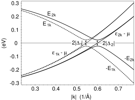
FIG. 1.: Dispersions in the normal state $\epsilon_{1k}$, $\epsilon_{2k}$ and quasi-particle dispersions in the superconducting state (T=0) in the $k$-region $|\epsilon_{k}|<\omega_{c}$. The parameters (22,23) are used.

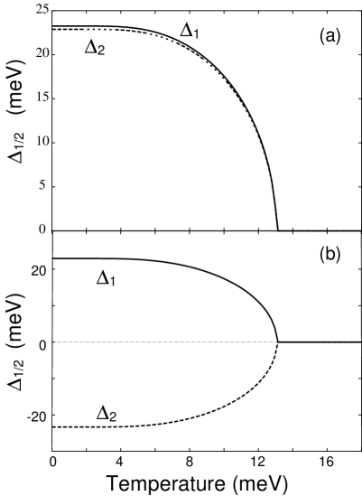
FIG. 2.: Gaps as function of temperature for negative (a) and positive interband coupling $\bar{V}$ (b). The parameters (22,23) are used.

We have chosen these values for the coupling constants in order to get $T_{c}$-values which are appropriate for high-T_c superconductors and ensure also the appearance of the collective modes we want to study.

Fig. 1 shows the dispersion for the two bands in the normal state and the quasi-particle dispersions in the superconducting state at zero temperature in the k-region $|\epsilon_{k}-\mu|<\omega_{c}$. Figures 2(a), 2(b) show the temperature dependence of the gaps for negative $\bar{V}$ (a) and positive $\bar{V}$ (b). Because the effective masses $m_{1}$ and $m_{2}$ are nearly the same (37) the values of the two gaps $\Delta_{1}$ and $\Delta_{2}$ are nearly the same. For repulsive interband coupling $\bar{V}$ the stable gaps have different signs. In both cases intralayer and interlayer pairing are mixed. But for negative $\bar{V}$ intralayer pairing dominates, for positive $\bar{V}$ interlayer pairing dominates. $T_{c}$ is 155 K. We have also calculated the level shifts $x_{i}$. They are practically temperature independent.

III Vertex equations

Now we will set up the integral equations for the vertex functions corresponding to the interlayer polarization and related operators defined in (16) for the neutral and charged system. We are interested in optical response functions for electric field vectors perpendicular to the layers. Here we can assume that the external wave vector is zero.

A Neutral system

We consider response functions where the bare vertex is one of the matrices $D^{jl}$, corresponding to the operators (16). In the standard ladder approximation the vertex equation for the renormalization of a vertex with matrix $D^{jl}$ reads

$$\Gamma^{jl}(i\omega_{s})=D^{jl}$$ (42)

$$-{1\over\beta}\sum_{k\omega_{n}}{\phantom{+}}VD^{03}G(k,i\omega_{n}+i\omega_{s})\Gamma^{jl}(i\omega_{s})G(k,i\omega_{n})D^{03}$$

$${\phantom{-{1\over\beta}\sum_{k\omega_{n}}}}+\bar{V}D^{13}G(k,i\omega_{n}+i\omega_{s})\Gamma^{jl}(i\omega_{s})G(k,i\omega_{n})D^{13}$$

$${\phantom{-{1\over\beta}\sum_{k\omega_{n}}}}+JD^{33}G(k,i\omega_{n}+i\omega_{s})\Gamma^{jl}(i\omega_{s})G(k,i\omega_{n})D^{33}$$

The vertex function depends only on the external frequency $\omega_{s}$, not on the momentum $k$ (apart from the cut-off) and the internal frequency of the Green’s function, because the interactions are assumed to be constant. The label $jl$ indicates to which bare vertex the vertex function belongs. In the case of the polarization we have to consider the matrix $D^{13}$. Of course, due to the interactions the renormalized vertex $\Gamma^{jl}$ contains also contributions from other matrices.

The interactions $V,J$ induce only intraband transitions, the interaction $\bar{V}$ only interband transitions. These interactions do not change the off-diagonal character of the bare vertices, therefore we can make the following ansatz for the renormalized vertex of the neutral system

$$\Gamma^{jl}=\left(\begin{array}[]{cc}0&\gamma\\ \hat{\gamma}&0\\ \end{array}\right)$$ (43)

with $2\times 2$ matrices $\gamma(i\omega_{s}),\hat{\gamma}(i\omega_{s})$. Then the system of vertex equations can be written as two coupled equations for $2\times 2$ matrices:

$$\gamma+W^{\prime}B+\bar{V}\hat{B} = I$$ (44)

$$\hat{\gamma}+W^{\prime}\hat{B}+\bar{V}B = \hat{I}$$ (45)

where $W^{\prime}=V-J=(V_{\parallel}+V_{\perp})/2-J$. The $2\times 2$ matrices $I$ and $\hat{I}$ are the upper right and lower left part of the matrix $D^{jl}$. In the case of the polarization $D^{13}$ we have $I=\sigma_{3}$, $\hat{I}=-\sigma_{3}$. The quantites $B$ are defined as

$$B(i\omega_{s})={1\over\beta}\sum_{\omega_{n}}\sum_{k}\sigma_{3}G_{1}(k,i\omega_{n}+i\omega_{s})\gamma(i\omega_{s})G_{2}(k,i\omega_{n})\sigma_{3}$$

$$\hat{B}(i\omega_{s})={1\over\beta}\sum_{\omega_{n}}\sum_{k}\sigma_{3}G_{2}(k,i\omega_{n}+i\omega_{s})\hat{\gamma}(i\omega_{s})G_{1}(k,i\omega_{n})\sigma_{3}$$ (46)

depending linearly on $\gamma(i\omega_{s})$. Note, that in contrast to the self-consistency equations (27, 29) ($W=V+J$) the interaction $J$ enters here with an other sign ($W^{\prime}=V-J$).

For the solution of this system of equations it is convenient to decompose $\gamma,\hat{\gamma}$ and also $B,\hat{B}$ into Pauli matrices:

$$\gamma=\gamma_{0}\sigma_{0}+\gamma_{1}\sigma_{1}+\gamma_{2}i\sigma_{2}+\gamma_{3}\sigma_{3}$$ (47)

$$B=B_{0}\sigma_{0}+B_{1}\sigma_{1}+B_{2}i\sigma_{2}+B_{3}\sigma_{3}$$ (48)

If we write the coefficient functions $\gamma_{i}$ as vector $\underline{\gamma}=(\gamma_{0},\gamma_{1},\gamma_{2},\gamma_{3})$ we can express the linear dependence of $B$ on these coefficients in matrix form:

$$\underline{B}=K\underline{\gamma},\quad\underline{\hat{B}}=\hat{K}\underline{\hat{\gamma}}$$ (49)

The $4\times 4$ matrices $K,\hat{K}$ are integrals over products of Green’s functions. For notational convenience it is useful to introduce an extra factor $i$ for the $\sigma_{2}$-component in (48). The structure of $K$ is given in the appendix (A3) and the functions are listed in (A7). With help of these matrices $K$, $\hat{K}$ the vertex equations can be written as

$$(1+W^{\prime}K)\underline{\gamma}+\bar{V}\hat{K}\underline{\hat{\gamma}} = \underline{I}$$ (50)

$$(1+W^{\prime}\hat{K})\underline{\hat{\gamma}}+\bar{V}K\underline{\gamma} = \underline{\hat{I}}$$ (51)

The matrix $\hat{K}$ differs from the matrix $K$ only by the sign of some elements in the first row and column. More precisely: $\hat{K}=gKg$ with $g$ being the diagonal matrix $g=diag(-1,1,1,1)$. $\underline{I}$ is a vector given by $(0,0,0,1)$, $(0,0,-i,0)$, $(0,1,0,0)$, $(-i,0,0,0)$ for $P^{13}$, $P^{12}$,$P^{11}$, $P^{20}$, respectively. $\underline{\hat{I}}$ fulfills: $\underline{\hat{I}}=g\underline{I}$. The second equation in (51) can be reduced to the first equation by setting

$$\underline{\hat{\gamma}}=g\underline{\gamma}$$ (52)

and it is sufficient to solve the first equation

$$\sum_{j}\left(\delta_{ij}+(W^{\prime}+\bar{V}g_{ii})K_{ij}\right)\gamma_{j}=I_{i}$$ (53)

which is a set of 4 linear equations.

A closer inspection of the integrals contained in the matrix $K$ shows that two of the integrals, $K_{11}$ and $K_{22}$ are badly convergent. They depend logarithmically on the cut-off in momentum space in a similar way as the integrals in the self-consistency equations (30). These badly convergent integrals can be eliminated by using relations (B19,B20) which can be derived from Ward identities. Then the cut-off is only needed in the calculation of the gaps $\Delta_{i}$.

The polarization function of the neutral system is given by

$$\ll P;P\gg_{i\omega_{s}}=$$ (55)

$${1\over\beta}\sum_{\omega_{n}}\sum_{k}Tr\{D^{13}G(k,i\omega_{n}+i\omega_{s})\Gamma^{13}(i\omega_{s})G(k,i\omega_{n})\}$$

The polarization function can be expressed by the matrix $B$ (46) or by the matrix $K$ using the commutation relations for the Pauli matrices and the development into Pauli matrices (48):

$$\ll P,P\gg=\ll P^{13},P^{13}\gg=4K_{3j}\gamma^{13}_{j}$$ (56)

B Charged system

Up to now we have only considered neutral superconductors. The long-range Coulomb interaction is known to have important consequences for the collective modes [1, 2, 3, 4]. Here we are interested in the optical properties for field vectors perpendicular to the layers in the long-wavelength limit $q\to 0$. Then we have to consider only the Coulomb interaction arising from charge fluctuations between the layers. These Coulomb forces stay finite in the long-wavelength limit but nevertheless are sizable. They can be incorporated in the vertex equations in a RPA-type manner.

Let $\Upsilon^{il}(i\omega_{s})$ be the vertex for the charged system. The vertex equation for $\Upsilon^{il}$ is obtained from the vertex of the neutral system (42), if $\Gamma^{jl}$ is replaced by $\Upsilon^{il}(i\omega_{s})$, and on the r.h.s. of the vertex equation (42) the following term is included:

$$D^{13}\bar{v}\sum_{\omega_{n}}\sum_{k}\,\,Tr\left\{D^{13}G(k,i\omega_{n}+i\omega_{s})\Upsilon^{jl}(i\omega_{s})G(k,i\omega_{n})\right\}$$ (57)

with $\bar{v}=\lim_{|q|\to 0}e^{2}\pi(1-{\rm e}^{-d|q|})/(|q|\epsilon_{0})=e^{2}\pi d/\epsilon_{0}$ the Coulomb interaction between the layers. For a periodic double-layer system $\bar{v}$ has to be replaced by $\pi e^{2}d(c-d)/c\epsilon_{0}$, where $d$ is the distance between the two layers in one unit cell and $c$ the distance between the unit cells. The vertex equation for $\Upsilon^{jl}$ can also be expressed by correlation functions and the vertex of the neutral system $\Gamma^{jl}$, as shown in Fig. 3. This equation reads:

$$\Upsilon^{jl}=\Gamma^{jl}+\Upsilon^{13}\bar{v}\ll P^{13},P^{jl}\gg$$ (58)

where the correlation function $\ll P^{13},P^{jl}\gg$ of the neutral system to which the interband Coulomb-interaction couples is given by:

$$\ll P^{13},P^{jl}\gg={1\over\beta}\sum_{\omega_{n}}\sum_{k}$$ (60)

$$Tr\{D^{13}G(k,i\omega_{n}+i\omega_{s})\Gamma^{jl}(i\omega_{s})G(k,i\omega_{n})\}$$

FIG. 3.: Diagrammatic representation of the vertex $\Upsilon^{jl}$ of the charged system with help of the vertex $\Gamma^{jl}$ (full circle) of the neutral system. The interband Coulomb-interaction $\bar{v}$ couples to the correlation function $\ll P^{13},P^{jl}\gg$ of the neutral system.

From this the vertex function $\Upsilon^{13}$ for the electronic polarization is easily calculated:

$$\Upsilon^{13}=\Gamma^{13}/(1-\bar{v}\ll P^{13},P^{13}\gg)$$ (61)

and we get for the polarization function for the charged system:

$$\ll P,P\gg_{i\omega_{s}}^{C}=\ll P,P\gg_{i\omega_{s}}/\left(1-\bar{v}\ll P,P\gg_{i\omega_{s}}\right)$$ (62)

IV Analytical discussion of the collective modes

In general the 4 vertex equations (53)

$$\sum_{j}\left(\delta_{ij}+(W^{\prime}+\bar{V}g_{ii})K_{ij}\right)\gamma_{j}=I_{i}$$ (63)

have to be solved numerically. But in some limits the equations can be simplified so that analytical results for the collective modes can be derived: 1. in the normal state and 2. in the limit of momentum independent tight-binding coupling $t_{k}$ between the layers.

In the following we need the special form of the matrix $K$ given in the Appendix:

$$K=\left(\begin{array}[]{cccc}H^{++}&-\tilde{Y}&-\tilde{Z}&\tilde{X}\\ \tilde{Y}&-H^{-+}&X&Z\\ \tilde{Z}&X&-H^{--}&Y\\ \tilde{X}&-Z&-Y&H^{+-}\\ \end{array}\right)$$ (64)

Furthermore we need the following combinations of coupling constants, which are listed here for completeness:

$$W=V+J,\quad W_{\parallel}=V_{\parallel}+J,\quad W_{\perp}=V_{\perp}-J$$ (65)

$$W^{\prime}=V-J,\quad W^{\prime}_{\parallel}=V_{\parallel}-J,\quad W^{\prime}_{\perp}=V_{\perp}-J$$ (66)

with $V=(V_{\parallel}+V_{\perp})/2,\quad\bar{V}=(V_{\parallel}+V_{\perp})/2$. Of special importance is the limit, where all pairing interactions are small

$$VN_{0},\,\,\,\bar{V}N_{0},\,\,\,JN_{0}\ll 1$$ (67)

This will be called the weak coupling limit in the following.

A Normal state

In the normal state the functions $Z,\,\,\tilde{Z},\,\,Y,\,\,\tilde{Y}$ vanish, because they are proportional to the gaps (A7). Therefore the set of equations (63) decouples. With $\underline{I}=(0,0,0,1)$ we obtain for the polarization vertex $\gamma=\gamma^{13}=\gamma^{P}$:

$$\gamma_{0} = -W^{\prime}_{\perp}\tilde{X}/N,\quad\gamma_{1}=\gamma_{2}=0,$$ (68)

$$\gamma_{3} = (1+W^{\prime}_{\perp}H^{++})/N$$ (69)

with $N=(1+W^{\prime}_{\perp}H^{++})(1+W^{\prime}_{\parallel}H^{+-})-W^{\prime}_{\parallel}W^{\prime}_{\perp}\tilde{X}^{2}$. The polarization function (56) is then given by

$$\ll P,P\gg_{i\omega_{s}}=4\left((1+W^{\prime}_{\perp}H^{++})H^{+-}-W^{\prime}_{\perp}(\tilde{X})^{2}\right)/N$$ (70)

In the case of momentum independent hopping ($t_{k}=t$) this expression can be simplified considerably by using the relations between the different matrix elements derived from the Ward identities (B18) and the approximation $(x_{2}-x_{1})/W_{\perp}=-2tN_{0}$. We obtain

$$\ll P;P\gg_{i\omega_{s}}=16N_{0}t^{2}(1+2N_{0}J)/M$$ (71)

with

$$M=(i\omega_{s})^{2}-4t^{2}[1-2(\bar{V}-2J)N_{0}-4J(\bar{V}-J)N_{0}^{2}]$$

The polarization function has a simple pole which is shifted with respect to the simple particle-hole excitation energy $2t$ due to the pairing interactions. In the weak coupling limit (67) we recover as result the bare polarization function, which is given by $H^{+-}$. In the charged system there exists then a plasmon describing interlayer charge fluctuations at $\omega^{2}=(2t)^{2}(1+\bar{v}N_{0})$.

B $k$-independent hopping matrix-element $t$

In the case of momentum independent tight-binding coupling ($t_{k}=t$) the solution for the self-consistency equations (29, 27) has the form

$$\Delta_{1}=\pm\Delta_{2}\quad{\rm and\ }x_{1}=-x_{2}$$ (72)

independent of the details of the band dispersion $\epsilon_{k}$. Then there exists a symmetry relation between the band dispersions $\xi_{1k}=\xi_{k}-t-x_{1}$ and $\xi_{2k}=\xi_{k}+t-x_{2}$ ($\xi_{k}=\varepsilon_{k}-\mu$) and the quasi-particle dispersions:

$$\xi_{2}(\xi_{k})=-\xi_{1}(-\xi_{k})$$ (73)

$$E_{1}(-\xi_{k})=E_{2}(\xi_{k})$$ (74)

Due to this symmetry some matrix functions $K_{ij}$ vanish and therefore (63) is reduced to a system of three coupled equations. We have to distinguish the two cases $\Delta_{1}=\pm\Delta_{2}$.

1 Intralayer pairing $\Delta_{1}=\Delta_{2}$

In the case of dominant intralayer interaction $W_{\parallel}$ the band gaps are equal ($\Delta_{1}=\Delta_{2}=\Delta_{\parallel}$) and interlayer pairing vanishes ($\Delta_{\perp}=(\Delta_{2}-\Delta_{1})/2=0$). Three functions are zero because of the relation (74):

$$Z(i\omega_{s})=X(i\omega_{s})=\tilde{Y}(i\omega_{s})=0$$ (75)

Therefore the second equation of the vertex equations (63) can be solved easily

$$\gamma_{1}^{j},\gamma_{1}^{\Phi},\gamma_{1}^{P}=0,\,\,\gamma_{1}^{A}(i\omega_{s})=1/\left(1-W_{\parallel}H^{-+}(i\omega_{s})\right),$$ (76)

$$\gamma_{l}^{A}=0,\,\,\,l=0,2,3$$ (77)

This means that oscillations of the amplitude $A$ do not couple to oscillations of the current $j$, polarization $P$, and phase $\Phi$. But the density, phase, and current oscillations couple to each other. The Coulomb interaction does not affect the amplitude fluctuations. This is in agreement with the results found in Refs. [13, 14], where a double layer system with $t=0$ is investigated. In the case of k-dependent hopping all these quantities couple, which will be demonstrated below by our numerical results.

The frequencies of the collective modes are determined by the zeros of the denominator of the vertex functions $\gamma^{jl}$. For the current, phase and polarization oscillations the frequency of the collective mode is given by the determinant of the corresponding $3\times 3$ matrix of the vertex-equation system (63); the collective mode of the amplitude oscillations is determined by (77).

The functions $K(\omega+i\delta)$ obtain imaginary parts at temperature $T=0$, when the frequency of the external field is large enough to break Cooper pairs ($\omega>min(E_{1k}+E_{2k})=\sqrt{(2\hat{t}\,)^{2}+(2\Delta_{\parallel})^{2}}$ with $\hat{t}=t+(x_{1}-x_{2})/2$). We are interested in undamped collective modes below the particle-hole threshold. In order to derive a simple approximation for the collective mode frequencies, we shall assume small frequencies $\omega\ll\sqrt{(2\hat{t}\,)^{2}+(2\Delta_{\parallel})^{2}}$, a small hopping matrix element $(\hat{t}/\Delta_{\parallel})^{2}\ll 1$ and zero temperature.

The functions $K$ (A7) can be evaluated with help of an expansion in $\hat{t}/\Delta_{\parallel}$ and $\omega/2\Delta_{\parallel}$:

$$H^{+-}(\omega)\approx-N_{0}+\omega^{2}C,\,\,H^{++}\approx(2\hat{t}\,)^{2}C$$ (78)

$$Y(\omega)\approx\omega\left(N_{0}+((2\hat{t}\,)^{2}-\omega^{2})C\right)/(2\Delta_{\parallel}),$$ (79)

$$\tilde{Z}(\omega)\approx-2\hat{N}_{0}/(2\Delta_{\parallel}),\,\,\tilde{X}\approx-\omega 2\hat{t}C$$ (80)

where $C=-N_{0}/(8\Delta_{\parallel}^{2})$. Here $-(x_{2}-x_{1})/(W_{\perp}2\hat{t}\,)$ has been approximated by the density of states at the Fermi level $N_{0}$ (see (32)).

With these expressions we expand the determinant up to second order in $\hat{t}/\Delta_{\parallel}$ or $\omega/(2\Delta_{\parallel})$

$$Det=\frac{N_{0}W_{\parallel}^{\prime}}{(2\Delta_{\parallel})^{2}}(1-\omega_{0}^{2}W_{\parallel}^{\prime}C)\left(\omega^{2}-\omega_{P}^{2}\right)$$ (81)

Here $\omega_{P}$ is the frequency of the collective phase mode in the neutral system

$$\omega_{P}^{2}=\left[\omega_{0}^{2}+(2\hat{t}\,)^{2}\left(1-W_{\perp}^{\prime}(N_{0}-\omega_{0}^{2}C)\right)\right]\frac{1-W_{\parallel}^{\prime}N_{0}}{1-\omega_{0}^{2}W_{\parallel}^{\prime}C}$$ (82)

$$\mbox{with}\quad\omega_{0}^{2}=\frac{(2\Delta_{\parallel})^{2}}{N_{0}}\,\frac{-2J}{V_{\parallel}^{2}-J^{2}}$$

This reduces to a simple result in the weak coupling limit (67):

$$\omega_{P}^{2}=(2t)^{2}+\omega_{0}^{2}$$ (83)

Because we have assumed small frequencies the formula is only valid for small $\omega_{0}$, i.e. $|J/V_{\parallel}|$ has to be small. The expression for the frequency $\omega_{0}$ has been derived already by Leggett [5]. Here we see how the mode-frequency is modified by the interlayer hopping $t$. It is justified to call this mode phase mode, because it appears as a resonance in the polarization function due to its coupling to the phase fluctuation.

Evaluating the polarization function (56) of the neutral system for small frequencies and small hopping matrix element we obtain

$$\ll P,P\gg_{\omega}=4N_{0}\frac{\omega_{P}^{2}(1-\omega_{0}^{2}W_{\parallel}^{\prime}C)-\omega^{2}\,\omega_{0}^{2}C\,(1-W_{\parallel}^{\prime}N_{0})}{\left(\omega^{2}-\omega_{P}^{2}\right)(1-\omega_{0}^{2}W_{\parallel}^{\prime}C)(1-W_{\parallel}^{\prime}N_{0})}$$ (84)

Inserting (84) into the polarization function with Coulomb interaction (62) we get the phase-mode frequency in the charged system:

$$\omega^{2}_{C}=\left[\omega_{0}^{2}+(2\hat{t}\,)^{2}\left(1-W_{\perp}^{\prime}(N_{0}-\omega_{0}^{2}C)\right)\right]$$ (85)

$$\times\frac{1+N_{0}(4\bar{v}-W_{\parallel}^{\prime})}{1+\omega_{0}^{2}C(4\bar{v}-W_{\parallel}^{\prime})}$$ (86)

In the weak coupling limit (67) and for small $|\omega_{0}^{2}C|$ we have

$$\omega_{C}^{2}=(\omega_{0}^{2}+(2t)^{2})(1+4N_{0}\bar{v})$$ (87)

The interband Coulomb interaction $\bar{v}$ shifts the mode up to higher frequencies. $\bar{v}$ is proportional to the distance $d$ between the layers. In order to get a phase mode below the particle hole threshold, it is necessary that the distance of the layers and the Josephson coupling constant $J$ is small. If the Josephson coupling $J$ is zero, the resonance appears at $2t$ as in the normal state but still below the particle-hole threshold. The mode corresponds to the collective tunneling of Cooper pairs between the layers without pair breaking.

The denominator of $\gamma_{1}^{A}$ (77) determines the amplitude mode. With the relations (B21) and using Ward identities (B18) we get:

$$\frac{1}{\gamma_{1}^{A}(\omega)}=1-\frac{W_{\parallel}^{\prime}}{W_{\parallel}}-\left(\frac{(2\hat{t}\,)^{2}-\omega^{2}}{(2\Delta_{\parallel})^{2}}+1\right)W_{\parallel}^{\prime}\frac{2\Delta_{\parallel}Y(\omega)}{\omega}$$ (88)

For vanishing Josephson coupling ($W_{\parallel}^{\prime}/W_{\parallel}=1$) the amplitude mode lies just at the particle-hole threshold:

$$\omega_{A}^{2}=(2\hat{t}\,)^{2}+(2\Delta_{\parallel})^{2}$$

For finite Josephson coupling an approximate analytical result can be obtained with (80):

$$\omega_{A}^{2}=(2\hat{t}\,)^{2}+2(\omega_{0}^{2}+(2\Delta_{\parallel})^{2})$$ (89)

Because we assumed small frequencies, this result is only valid, if $\omega_{0}^{2}$ is negative, which is obtained for positive $J$. For the general solution we refer to the numerical calculation.

The formula for the phase (83) and amplitude mode (89) show how the mode frequencies are shifted by the hopping $t$ and the results of Refs.[5, 13] are modified. Note, however, that the particle-hole threshold is shifted too.

2 Interlayer pairing $\Delta_{1}=-\Delta_{2}$

In the case of dominant interlayer interaction, when $\Delta_{\perp}=(\Delta_{2}-\Delta_{1})/2\neq 0,\,\,\Delta_{\parallel}=(\Delta_{2}+\Delta_{1})/2=0$, the following three functions are zero because of (74):

$$\tilde{Z}(i\omega_{s})=X(i\omega_{s})=Y(i\omega_{s})=0$$ (90)

The third column and line of the vertex equation matrix (63) is zero with the exception of the diagonal element. Now the oscillations of $\Phi$ are decoupled from the the oscillations of the other quantities, while $j$, $A$ and $P$ couple to each other.

Again we study the limit of small frequencies $\omega\ll\sqrt{(2\hat{t}\,)^{2}+\Delta_{\perp}^{2}}$ and small hopping $|\hat{t}/\Delta_{\perp}|^{2}\ll 1$. The functions can be approximated as:

$$H^{++}\approx-N_{0}+\omega^{2}C,\,\,H^{+-}\approx(2\hat{t}\,)^{2}C,$$ (91)

$$\tilde{Y}\approx\omega(N_{0}+((2\hat{t}\,)^{2}-\omega^{2})C)/(2\Delta_{\perp}),$$ (92)

$$Z\approx-2\hat{t}N_{0}/(2\Delta_{\perp}),\,\,\tilde{X}\approx-\omega 2\hat{t}C,$$ (93)

$$H^{-+}\approx 1/W_{\perp}-(\omega^{2}-(2\hat{t}\,)^{2})N_{0}/(2\Delta_{\perp})$$ (94)

where $C=-N_{0}/8\Delta_{\perp}^{2}$ and $\hat{t}=t+(x_{1}-x_{2})/2$ as before. From the vanishing of the determinant of the three coupled equations we now obtain for the frequency of the collective mode determining polarization and amplitude oscillations:

$$\omega_{P}^{2}=\left[\omega_{0}^{2}+(2\hat{t}\,)^{2}\left(1-W_{\parallel}^{\prime}(N_{0}-\omega_{0}^{2}C)\right)\right]\frac{1-W_{\perp}^{\prime}N_{0}}{1-\omega_{0}^{2}W_{\perp}^{\prime}C}$$ (95)

with

$$\omega_{0}^{2}=\frac{(2\Delta_{\perp})^{2}}{N_{0}}\,\frac{2(\bar{V}-J)}{V^{2}-(\bar{V}-J)^{2}}$$

In the week coupling limit (67) the mode in the neutral system becomes:

$$\omega_{P}^{2}=(2t)^{2}+\omega_{0}^{2}$$ (96)

Expanding the nominator and denominator of the polarization function (56) up to second order in $\hat{t}/\Delta_{\perp}$ and $\omega/2\Delta_{\perp}$ we obtain

$$\ll P,P\gg_{\omega}=4(N_{0}-\omega_{0}^{2}C)\frac{(2\hat{t}\,)^{2}(1-W_{\perp}^{\prime}N_{0})}{\left(\omega^{2}-\omega_{P}^{2}\right)(1-\omega_{0}^{2}W_{\perp}^{\prime}C)}$$ (97)

In this case the polarization function is zero, if the single-particle hopping $t$ vanishes. This is in contrast to the case of intralayer pairing, where the pair tunneling due to $J$ produces density fluctuations between the layers and therefore spectral weight in the polarization function even in the absence of single-particle hopping. P. W. Anderson argues that due to correlations the single-particle hopping is suppressed. If this is right, then in the case of interlayer pairing no excitation of charge fluctuations between the layers should be seen in the optical c-axes conductivity $\sigma(\omega)$, which is related to the polarization function by: $\sigma(\omega+i\delta)=i\omega<<P,P>>_{\omega+i\delta}(ed/2)^{2}$.

The collective mode in the charged system is given by:

$$\omega^{2}_{C} = \left[\omega_{0}^{2}+(2\hat{t}\,)^{2}\left(1+(4\bar{v}-W_{\parallel}^{\prime})(N_{0}-\omega_{0}^{2}C)\right)\right]$$ (99)

$$\quad\times\,\,\frac{1-W_{\perp}^{\prime}N_{0}}{1-\omega_{0}^{2}W_{\perp}^{\prime}C}$$

Only the term containing the single-particle hopping is influenced by the Coulomb interaction. This is consistent with the picture of interlayer pairing. The hopping of interlayer Cooper-pairs produces no charge fluctuation between the layers. When an interlayer pair is tunneling, one electron jumps to the upper layer, the other to the lower layer and the charge density on the layers does not change.

In a similar way as above we obtain for the frequency of the phase mode, which is now decoupled from the polarization:

$$\omega_{\Phi}^{2}=(2\hat{t}\,)^{2}+2(\omega_{0}^{2}+(2\Delta_{\perp})^{2})$$ (100)

Because we assumed small frequencies, this result is only valid, if $\omega_{0}^{2}$ is negative, which is obtained for negative $\bar{V}-J$. For the general solution we refer to the numerical calculation.

In comparison to the case of intralayer pairing the modes have changed their role. The amplitude mode is now the low lying excitation and is coupled to the electronic polarization. As in the ground state of interlayer pairing the layer order-parameters $<c_{1\uparrow}c_{1\downarrow}>$ and $<c_{2\uparrow}c_{2\downarrow}>$ are zero it is no longer justified to call oscillations of $\Phi$ phase oscillations. We kept this name for convenience only.

V numerical results

In the general case of k-dependent hopping when intralayer and interlayer pairing are mixed it is not possible to derive simple expressions for the dispersions of the collective modes. We made numerical calculations for the polarization functions with the dispersion parameters (37) and coupling constants

$$N_{0}W=-0.139,\quad N_{0}\bar{V}=\pm 0.185,\quad N_{0}\bar{v}=1.3$$ (101)

for constant $W=V+J$ and variable Josephson coupling $J$ for dominating intralayer ($\bar{V}<0$) and interlayer pairing ($\bar{V}>0$), in order to study the influence of the Josephson coupling $J$ and the temperature dependence of the collective modes. We present results both for the neutral system and taking into account the Coulomb interaction $\bar{v}$ between the layers. To resolve the $\delta$-peaks of the collective modes at $T=0$ below the particle-hole threshold we have introduced a small imaginary part ($10^{-3}$ meV) to the frequency.

A Dominant intralayer pairing

First we discuss the results for the case of dominant intralayer pairing ($\bar{V}<0,\Delta_{1}\Delta_{2}>0$). In Fig. 4 the spectrum of the collective modes (sharp spikes) and the form of the particle-hole spectrum at $T=0$ is shown. The imaginary parts of the polarization function in the

FIG. 4.: Imaginary parts of the polarization function in the neutral (a) and charged (b) system at $T=0$ in the case of dominant intralayer pairing for different Josephson couplings $J$. The parameter sets (22,23) are used. The results are normalized by $\bar{N}_{0}=13N_{0}$. The different lines are shifted by equal units. The rhombs, crosses, and dashed lines in the figures correspond to various approximation formulas for the collective mode frequencies discussed in the text.

neutral 4(a) and the charged system 4(b) are calculated for different Josephson couplings $J$ and constant intraband $W=V+J$ and interband coupling $\bar{V}$. For comparison results of the approximation formulas are plotted, too. The rhombs and crosses in (a) refer to the formulas for the phase (82) and amplitude mode (89), respectively, calculated with a constant averaged hopping $t=-30.5\,{\rm meV}$. The dashed line represents the phase mode frequency (83) in the weak coupling limit.

For negative Josephson couplings $J$ a collective mode, the phase mode, lies just below the particle-hole threshold. With increasing positive $J$ the phase-mode peak moves to lower frequencies.

For positive $J$ another mode, the amplitude mode, becomes visible near the particle-hole threshold. For increasing $J$ the peak moves to smaller frequencies. Thus, two superconducting collective modes can occur in the polarization function perpendicular to the layers. This effect is caused by the coupling of the phase and amplitude fluctuations.

The two approximation formulas for the phase mode, represented by the rhombs and the dashed line, give qualitatively the right position of the collective-mode frequencies, as long as the peaks are below the particle-hole threshold. The same holds for the approximated values for the amplitude mode (crosses).

For $N_{0}J\geq 0.06$ the peak of the phase mode has passed zero, and its frequency has become imaginary. This behaviour is also obtained by using the approximation formula (83). We believe, that this instability indicates a phase transition from intraband to interband pairing. This is supported by a study of a two-site model with two electrons (see section self-consistency equation), where a strong positive coupling $J$ leads to a ground state consisting of interband Cooper-pairs ($a^{\dagger}_{1\uparrow}a^{\dagger}_{2\downarrow}$).

In Fig. 4(b) the influence of the Coulomb interaction between the layers is shown. A plasmon exists within the particle-hole continuum. This mode is caused by charge fluctuations between the layers. The damping of this mode increases with increasing $|J|$. The particle-hole threshold peak is strongly suppressed, if there exists a collective mode with large spectral weight above the threshold. Again the approximation formula for the phase mode in the weak coupling limit, represented by the dashed line in Fig. 4(b), gives the right position of the plasmon peak for small $|J|$. The plasmon mode and phase mode coincide for small $|J|$.

But for positive $J$ a peak below the particle-hole threshold appears ($N_{0}J=0.02,\,\,\,0.04$). This peak can be attributed to phase fluctuations by comparing the peak positions with the analytical results obtained for constant $t$ (rhombs). The amplitude peak lies just at the particle-hole threshold at $N_{0}J=0.04$ and can be seen at $N_{0}J=0.06$. Those peaks which we have attributed to the phase and amplitude modes have large spectral weight in the correlations functions $\ll\Phi,\Phi\gg$ and $\ll A,A\gg$, respectively.

Now we discuss the temperature dependence of the polarization functions for large positive (0.05) and negative (-0.06) Josephson coupling.

Fig. 5 shows the imaginary part of the bare polarization function (a), the polarization function in the neutral system (b), and the real part of the optical

FIG. 5.: Imaginary parts of the bare polarization function (a), the polarization function in the neutral system (b), and the real part of the optical conductivity in the charged system (c) in the case of dominant intralayer pairing for different temperatures $T$ and positive Josephson coupling $N_{0}J=0.05$. The parameters (22,23) are used. The different lines are shifted by equal units. In (c) we choose as distance between the layers $d=3\AA$.

conductivity in the charged system (c). The latter is related to the polarization function by $\sigma(\omega+i\delta)=i\omega(ed/2)^{2}\ll P,P\gg_{\omega+i\delta}^{C}$. In picture 5(a) only particle-hole excitations with energy $|E_{1k}+E_{2k}|$ are visible at $T=0$. For finite temperatures also excitations with $|E_{1k}-E_{2k}|$ from excited levels are possible at lower frequencies. The broad peak at $T_{c}$ is due to interband transitions with different $t_{k}$-values. The Fig. 5(b) shows the complicated transition from two distinct collective modes at $T=0$ (phase and amplitude mode) to a collective density fluctuation in the normal state. The Coulomb interaction between the layers shifts the collective modes associated with density fluctuations to higher frequencies (Fig. 5(c)), whereas the amplitude mode near the particle-hole threshold is only slightly shifted.

FIG. 6.: Real part of the optical conductivity $\sigma(\omega)$ in the case of dominant intralayer pairing for different temperatures $T$ and negative Josephson coupling $N_{0}J=-0.06$. The parameters (22,23) are used, $d=3\AA$. The different lines are shifted by equal units.

In the case of negative $J$, which is the more realistic one, if this coupling is produced by the exchange of a boson, the Coulomb interaction shifts the collective modes into the region of particle-hole excitations. Fig. 6 shows the temperature dependence of the remaining density-fluctuation spectrum.

B Dominant interlayer pairing

In the case of dominant interlayer pairing ($\bar{V}>0,\Delta_{1}\Delta_{2}<0$) it is possible to produce the same peak structures in the polarization function as in the case of dominant intralayer pairing. Fig. 7 shows the imaginary parts of the polarization function in the neutral (a) and charged (b) system for selected $J$-values. The structures are nearly the same as in Fig. 4. For $J$ greater equal $\bar{V}$ collective modes below the particle-hole threshold can occur in the polarization function of the neutral system and for relative large positive $J$ also in the polarization function for the charged system. The damping behavior of the plasmon is quite similar as in the case of dominant intralayer pairing. For negative and small positive $J$ the plasmon peak is strongly damped.

FIG. 7.: Imaginary part of the polarization function in the neutral (a) and charged (b) system in the case of dominant interlayer pairing for different Josephson couplings and temperature $T=0$. The parameters (22,23) are used.

An example for the temperature dependence of the imaginary part of the polarization function in the neutral (full lines) and charged (dashed lines) system shows Fig. 8. The plasmon (dashed line) has the same behaviour as in Fig. 6.

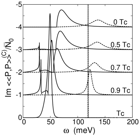
FIG. 8.: Imaginary part of the polarization function in the neutral (full lines) and charged (dashed lines) system in the case of dominant interlayer pairing for different temperatures and Josephson coupling $J=0$. The parameters (22,23) are used.

VI Conclusions

In this paper we have studied collective modes in superconducting double-layer systems which are connected with charge fluctuations between the layers. In our model we assumed a single-particle tight-binding hopping $t_{k}$ between the layers and considered three different types of pairing interactions: an intralayer interaction $V_{\parallel}$, an interlayer interaction $V_{\perp}$ and a Josephson-type coupling $J$ which allows a transfer of two particles between the layers. With these interactions we set up a system of vertex equations within a conserving approximation. The collective modes then appear as resonances in the vertex functions. So we were able to study the interplay of the three types of interlayer interactions $t_{k}$, $V_{\perp}$, and $J$, which has not been investigated so far together.

Due to the interaction $V_{\perp}$ Cooper pairs with electrons in different layers are formed. Depending on the relative size of the different interactions one finds dominating interlayer or intralayer pairing. In the case of constant hopping $t$ we calculated analytically the frequency of the collective modes. It is of the form $\omega=\sqrt{(2t)^{2}+\omega_{0}^{2}}$ in the neutral system. In the case of intralayer pairing $\omega_{0}^{2}$ is proportional to the ratio $-J/|V_{\parallel}|$ while for interlayer pairing it is proportional to $(V_{\parallel}-V_{\perp}-2J)/|V_{\parallel}+V_{\perp}|$ (in the limit that theses ratios are small). The former result is in agreement with the result for the collective mode obtained by Wu and Griffin [13] for $t=0$. The latter result is new. In order to find an undamped collective mode it is important that its frequency is below the particle hole threshold $\sqrt{(2t)^{2}+(2\Delta)^{2}}$. As for realistic systems $\omega_{0}^{2}>0$ the best chances to observe a collective mode is for the case of intralayer pairing and small Josephson coupling $J$. However, one has to keep in mind that the Coulomb interaction between the layers leads to a further shift to higher frequencies. This Coulomb interaction is proportional to the distance between the layers but can be reduced by a large phononic polarizability of the intermediate layers.

In principle one has to distinguish two different modes which in the literature sometimes are called phase and amplitude mode. For $\omega_{0}^{2}<0$ the two collective modes, can both have frequencies below the particle-hole threshold for the same coupling parameters in the neutral system. However, in the case of constant $t$ and equal values of the two gaps (pure intralayer or interlayer pairing) only one of these modes couples to the electronic polarization and will show up in the optical spectra. This is different for mixed intralayer and interlayer pairing and finite hopping (this occurs in our model for k-dependent hopping $t_{k}$). Then both phase and amplitude oscillations couple to the charge oscillation between the layers. Therefore in the c-axis optical conductivity two collective mode peaks can appear below the particle-hole threshold for low enough Coulomb interaction.

For a more realistic parameter region (negative $J$ and strong Coulomb interaction) only one collective mode, the plasmon corresponding to charge fluctuations between the layers, exists. In this case most of the weight of the polarization spectrum is concentrated in the plasmon peak; the particle-hole excitations and in particular the peak at the threshold of particle-hole excitations are strongly suppressed. Therefore it is difficult to determine the threshold energy for breaking up Cooper pairs or the superconducting gap with optical c-axis experiments. It is remarkable that the plasmon peak is much narrower in the normal state than in the superconducting state. That is due to the stronger quasiparticle dispersion in the superconducting state, allowing a much wider range of interband transition energies.

Up to now the c-axis plasmon is not detected in the layered high-$\rm T_{c}$ superconductors YBCO or BSCCO. One explanation could be, that in these compounds the single-particle hopping $t$ is zero (suppressed by correlation effects, as suggested by P.W. Anderson) and furthermore interlayer pairing dominates. The fluctuation of interlayer Cooper-pairs does not produce density fluctuations between the layers. The weight of the polarization function would then only be determined by the hopping matrix-element and therefore vanishes. But it is also possible (not investigated here) that the plasmon is overdamped by impurity scattering [26] or more likely by inelastic scattering effects at high frequencies due to antiferromagnetic spin fluctuations.

A Matrix Elements

For the matrix $K_{ij}$ we have to calculate the following integrals:

$$K_{ij}={1\over\beta}\sum_{\omega_{n}k}\frac{1}{2}Tr\left\{\bar{\sigma}_{i}^{T}\sigma_{3}G_{1}(k,i\omega_{n}+i\omega_{s})\bar{\sigma}_{j}G_{2}(k,i\omega_{n})\sigma_{3}\right\}$$ (A1)

where $\sigma_{i}$ are Pauli matrices and the matrices $\bar{\sigma}_{j}$ are defined by:

$$\bar{\sigma}_{j}=\sigma_{j}\quad{\rm for\,\,}j=0,1,3,\quad\bar{\sigma}_{2}=i\sigma_{2},\quad\bar{\sigma}_{2}^{T}=-i\sigma_{2}$$

Defining the integrals

$$H^{\pm\pm}(i\omega_{s})={1\over\beta}\sum_{\omega_{n}}\sum_{k}[(i\omega_{n}+i\omega_{s})i\omega_{n}\pm\xi_{1k}\xi_{2k}\pm\Delta_{1}\Delta_{2}]/N$$

$$(X/\tilde{X})(i\omega_{s})={1\over\beta}\sum_{\omega_{n}}\sum_{k}[(i\omega_{n}+i\omega_{s})\xi_{2k}\mp i\omega_{n}\xi_{1k}]/N$$

$$(Y/\tilde{Y})(i\omega_{s})={1\over\beta}\sum_{\omega_{n}}\sum_{k}[(i\omega_{n}+i\omega_{s})\Delta_{2}\mp i\omega_{n}\Delta_{1}]/N$$

$$(Z/\tilde{Z})(i\omega_{s})={1\over\beta}\sum_{\omega_{n}}\sum_{k}[\xi_{1k}\Delta_{2}\pm\xi_{2k}\Delta_{1}]/N$$ (A2)

with

$$N=[(i\omega_{n}+i\omega_{s})^{2}-E^{2}_{1k}][(i\omega_{n})^{2}-E^{2}_{2k}]$$

The matrix $K$ can be written as

$$K=\left(\begin{array}[]{cccc}H^{++}&-\tilde{Y}&-\tilde{Z}&\tilde{X}\\ \tilde{Y}&-H^{-+}&X&Z\\ \tilde{Z}&X&-H^{--}&Y\\ \tilde{X}&-Z&-Y&H^{+-}\\ \end{array}\right)$$ (A3)

The different signs come from the commutation relations for the Pauli matrices. Integrals of this type are common in vertex equations for superconductors [24] and for antiferromagnetic systems [25].

The frequency summations are all of the general form

$$J(k,i\omega_{s})={1\over\beta}\sum_{\omega_{n}}{F(i\omega_{n}+i\omega_{s},i\omega_{n})\over((i\omega_{n}+i\omega_{s})^{2}-E_{1k}^{2})((i\omega_{n})^{2}-E^{2}_{2k})}$$ (A4)

where the functions $F(z_{1},z_{2})$ are given by

$$H^{\pm\pm}: F(z_{1},z_{2}) =z_{1}z_{2}\pm\xi_{1k}\xi_{2k}\pm\Delta_{1}\Delta_{2}$$ (A5)

$$(X/\tilde{X}): F(z_{1},z_{2}) =z_{1}\xi_{2k}\mp z_{2}\xi_{1k}$$ (A6)

$$(Y/\tilde{Y}): F(z_{1},z_{2}) =z_{1}\Delta_{2}\mp z_{2}\Delta_{1}$$ (A7)

$$(Z/\tilde{Z}): F(z_{1},z_{2}) =\xi_{1k}\Delta_{2}\pm\xi_{2k}\Delta_{1}$$ (A8)

After performing the frequency summations with help of Poisson’s summation formula we obtain:

$$J(k,i\omega_{s} ) ={1\over 8E_{1k}E_{2k}}\left(\tanh{\beta E_{1k}\over 2}+\tanh{\beta E_{2k}\over 2}\right)$$ (A9)

$$\times \left({F(-E_{1k},E_{2k})\over i\omega_{s}+E_{1k}+E_{2k}}-{F(E_{1k},-E_{2k})\over i\omega_{s}-E_{1k}-E_{2k}}\right)$$ (A10)

$$+ {1\over 8E_{1k}E_{2k}}\left(\tanh{\beta E_{1k}\over 2}-\tanh{\beta E_{2k}\over 2}\right)$$ (A11)

$$\times \left({F(E_{1k},E_{2k})\over i\omega_{s}-E_{1k}+E_{2k}}-{F(-E_{1k},-E_{2k})\over i\omega_{s}+E_{1k}-E_{2k}}\right)$$ (A12)

One notices that the first term containing contributions from the creation or destruction of two quasi-particles in different bands remains finite also for $T\to 0$. The second term with transfer of quasi-particles from one band to the other vanishes in that limit. Using the expressions for the function $F(z^{\prime},z)$ the different matrix-elements are easily calculated. One observes that the integrals $H^{\pm\pm},Z,\tilde{Z}$ are even functions of $\omega_{s}$ while the integrals $X,\tilde{X},Y,\tilde{Y}$ are odd functions.

B Vertex Functions and Ward Identities

We derive some useful relations between different integrals of the matrix $K$, which are based on the conserving approximation used for the calculation of self-energies and vertex-functions. Similar relations for a one-band system are calculated e.g. in Ref [6].

The vertex equation in the neutral system in ladder approximation has the general form (42).

$$\Gamma^{jl}(i\omega_{s})=D^{jl}-L\{\Gamma^{ij}\}$$ (B1)

with

$$L\{\Gamma\}={1\over\beta}\sum_{\omega_{n}k}{\phantom{+}}$$ (B5)

$${\phantom{+}}VD^{03}G(k,i\omega_{n}+i\omega_{s})\Gamma(i\omega_{s})G(k,i\omega_{n})D^{03}$$

$$+\bar{V}D^{13}G(k,i\omega_{n}+i\omega_{s})\Gamma(i\omega_{s})G(k,i\omega_{n})D^{13}$$

$$+JD^{33}G(k,i\omega_{n}+i\omega_{s})\Gamma(i\omega_{s})G(k,i\omega_{n})D^{33}$$

We consider only vertex functions $\Gamma$, which are off-diagonal in the band indices:

$$\Gamma=\left(\begin{array}[]{cc}0&\gamma\\ \hat{\gamma}&0\\ \end{array}\right)$$ (B6)

Then $L$ is also off-diagonal in the band indices and can be written as

$$L=\left(\begin{array}[]{cc}0&\lambda\\ \hat{\lambda}&0\\ \end{array}\right)$$ (B7)

Now let us define a k-dependent vertex function:

$$\Gamma^{a}_{k}(i\omega_{s})=G^{-1}(k,i\omega_{n}+i\omega_{s})D^{13}-D^{13}G^{-1}(k,i\omega_{n})$$ (B8)

then the right upper corner is:

$$\gamma^{a}_{k}=i\omega_{s}\sigma_{3}+2\hat{t}_{k}\sigma_{0}-i(\Delta_{1}+\Delta_{2})\sigma_{2}$$ (B9)

where $\hat{t}_{k}=(\xi_{2k}-\xi_{1k})/2$.

Inserting $\Gamma^{a}$ into the r.h.s. of (B2) some of the Green’s function cancel, and the integrals are reduced to those which also occur in the self-energies (24). In particular we obtain for the $2\times 2$ matrix in the right upper corner

$$\lambda^{a} = \sum_{k}\sum_{\omega_{n}}\ W^{\prime}\left(G_{2}(k,i\omega_{n})\sigma_{3}-\sigma_{3}G_{1}(k,i\omega_{n}+i\omega_{s})\right)$$

$${\phantom{\sum_{k}\sum_{\omega_{n}}}}+\bar{V}\left(G_{1}(k,i\omega_{n})\sigma_{3}-\sigma_{3}G_{2}(k,i\omega_{n}+i\omega_{s})\right)$$

$$= \frac{1}{W^{2}-{\bar{V}}^{2}}$$

$$\times \Big{\{}\,\,\,W^{\prime}\left[\sigma_{3}(-W\Sigma_{2}+\bar{V}\Sigma_{1})+(W\Sigma_{1}-\bar{V}\Sigma_{2})\sigma_{3}\right]$$

$$+\bar{V}\left[\sigma_{3}(-W\Sigma_{1}+\bar{V}\Sigma_{2})+(W\Sigma_{2}-\bar{V}\Sigma_{1})\sigma_{3}\right]\Big{\}}$$

$$=\frac{W^{\prime}+\bar{V}}{W+\bar{V}}(\Delta_{2}+\Delta_{1})i\sigma_{2}+\frac{W^{\prime}-\bar{V}}{W-\bar{V}}(x_{2}-x_{1})\sigma_{0}$$ (B10)

On the other hand we can calculate $L\{\Gamma\}$ in an other way. With the quantities $B$ and $\hat{B}$ defined in (46) $\lambda$ is given by:

$$\lambda^{a}=W^{\prime}B+\bar{V}\hat{B}$$ (B11)

Because of the $k$-dependence of the vertex function $\gamma^{a}_{k}$ we introduce the $k$-dependent $4\times 4$ matrix functions $K_{k}$ and $\hat{K}_{k}$, which are related to $K$ and $\hat{K}$ by

$$K=\sum_{k}K_{k},\quad\hat{K}=\sum_{k}\hat{K}_{k}$$

The same relations we needed for deriving the vertex equation (63) holds for the $k$-dependent quantities $K_{k}$, $\hat{K}_{k}$, $\gamma^{a}_{k}$, and $\hat{\gamma}^{a}_{k}$. Therefore we find:

$$\underline{\lambda}^{a}=(W^{\prime}+g\bar{V})\sum_{k}K_{k}\underline{\gamma}^{a}_{k}$$ (B12)

where $g$ is the diagonal matrix $g=diag(-1,1,1,1)$. Thus we arrive at the first identity:

$$(W+g\bar{V})\sum_{k}K_{k}\underline{\gamma}^{a}_{k}=(x_{2}-x_{1},0,\Delta_{2}+\Delta_{1},0)^{t}$$ (B13)

Note on the l.h.s. stands $W$ not $W^{\prime}$, because the factor $W^{\prime}+g\bar{V}$ cancels.

In a similar way we find a second relation starting from

$$\Gamma_{k}^{b}(i\omega_{s})=G^{-1}(k,i\omega_{n}+i\omega_{s})D^{10}-D^{10}G^{-1}(k,i\omega_{n})$$ (B14)

Inserting this into the integral $L$ we obtain

$$\lambda^{b} = \sum_{k}\sum_{\omega_{n}}W^{\prime}\sigma_{3}G_{2}(k,i\omega_{n})\sigma_{3}-\bar{V}\sigma_{3}G_{1}(k,i\omega_{n})\sigma_{3}$$

$$-W^{\prime}\sigma_{3}G_{1}(k,i\omega_{n}+i\omega_{s})\sigma_{3}+\bar{V}\sigma_{3}G_{2}(k,i\omega_{n}+i\omega_{s})\sigma_{3}$$

$$={W^{\prime}+\bar{V}\over W-\bar{V}}(\Sigma_{1}-\Sigma_{2})$$ (B15)

or

$$\sum_{k}K_{k}\underline{\gamma}_{k}^{b}={1\over W-\bar{V}}(0,(\Delta_{2}-\Delta_{1}),0,-(x_{2}-x_{1}))^{t}$$ (B16)

In the case of vanishing Josephson coupling and k-independent hopping $t$ the first relation is identical with the Ward identity

$$i\omega_{s}\Gamma^{P}+2it\Gamma^{j}=\Gamma^{a}_{k}$$ (B17)

which follows from the continuity equation $2tj=\dot{P}$ (compare the discussion to (16)). $\Gamma^{P}$ is here the polarization vertex and $\Gamma^{j}$ the current vertex. The second relation is not a Ward identity based on a conservation law. It is valid only within the ladder approximation for the vertex equation. More relations are obtained by replacing the matrix $D^{13}$ by $D^{11}$ or $D^{12}$. These relations, however, are not of practical use.

From the above relations we obtain the following identities between the different integrals:

$$\begin{array}[]{ccccccc}2H^{t++}&+&\tilde{Z}2\Delta_{\parallel}&+&\tilde{X}i\omega_{s}&=&(x_{2}-x_{1})/W_{\perp}\\ 2\tilde{Y}^{t}&-&X2\Delta_{\parallel}&+&Zi\omega_{s}&=&0\\ 2\tilde{Z}^{t}&+&H^{--}2\Delta_{\parallel}&+&Yi\omega_{s}&=&2\Delta_{\parallel}/W_{\parallel}\\ 2\tilde{X}^{t}&+&Y2\Delta_{\parallel}&+&H^{+-}i\omega_{s}&=&0\\ H^{++}i\omega_{s}&+&\tilde{Y}2\Delta_{\perp}&+&2\tilde{X}^{t}&=&0\\ \tilde{Y}i\omega_{s}&+&H^{-+}2\Delta_{\perp}&+&2Z^{t}&=&2\Delta_{\perp}/W_{\perp}\\ \tilde{Z}i\omega_{s}&-&X2\Delta_{\perp}&+&2Y^{t}&=&0\\ \tilde{X}i\omega_{s}&+&Z2\Delta_{\perp}&+&2H^{t+-}&=&(x_{2}-x_{1})/W_{\perp}\end{array}$$ (B18)

where $W_{\parallel}=V_{\parallel}+J=W+\bar{V}$, $W_{\perp}=V_{\perp}+J=W-\bar{V}$ and $\Delta_{\parallel}=(\Delta_{2}+\Delta_{1})/2,\Delta_{\perp}=(\Delta_{2}-\Delta_{1})/2$. Here the quantities $K^{t}_{ij}$ are integrals similar to $K_{ij}$ with the integrand multiplied by $\hat{t}_{k}=t_{k}+(x_{1}-x_{2})/2$ before the momentum integration. In the case of momentum independent hopping matrix-element $t_{k}$ we have $K^{t}_{ij}=\hat{t}K_{ij}$.

The identities can be used to eliminate the badly converging integrals $H^{-+}$ and $H^{--}$:

$$H^{-+} = \frac{1}{W_{\perp}}-{1\over\Delta_{2}-\Delta_{1}}(i\omega_{s}\tilde{Y}+2Z^{t})$$ (B19)

$$H^{--} = \frac{1}{W_{\parallel}}-{1\over\Delta_{1}+\Delta_{2}}(i\omega_{s}Y+2\tilde{Z}^{t})$$ (B20)

Here the integrals on the r.h.s. do not need a cut-off.

In the two special cases of pure intralayer and interlayer pairing one can derive from the definitions of the functions (A7) two further relations:

$$H^{-+}=H^{--}+(\Delta_{1}+\Delta_{2})Y/i\omega_{s}\quad\mbox{if\ }\Delta_{1}=\Delta_{2}$$ (B21)

$$H^{--}=H^{-+}+(\Delta_{2}-\Delta_{1})\tilde{Y}/i\omega_{s}\quad\mbox{if\ }\Delta_{1}=-\Delta_{2}$$ (B22)

REFERENCES

• [1] P. W. Anderson, Phys. Rev. 110, 827 (1958), 1900 (1958); N. N. Bogoliubov, Nuovo Cimento 7, 794 (1958).
• [2] J. R. Schrieffer ”Superconductivity” (Benjamin, New York, 1964).
• [3] Y. Nambu, Phys. Rev. 117, 648 (1960).
• [4] P. Martin, in ”Superconductivity”, edited by R. D. Parks (Dekker, New York, 1969), pp. 371-379.
• [5] A. J. Leggett, Progr. Theor. Phys. (Japan) 36, 901 (1966).
• [6] P. B. Littlewood, C. M. Varma, Phys. Rev. B 26, 4883 (1982).
• [7] P. J. Hirschfeld, W. O. Puttika, P. Wölfle, Phys. Rev. Lett. 69, 1447 (1992).
• [8] H. Monien, L. Tewordt, K. Scharnberg, Solid State Commun. 63, 1027 (1987).
• [9] P. Wölfle, J. Low Temp. Phys. 95, 191 (1994).
• [10] H. A. Fertig, S. Das Sarma, Phys. Rev. B 44, 4480 (1991); R. Côtè, A. Griffin, Phys. Rev. B 48, 10404 (1993).
• [11] O. K. Andersen, O. Jepsen, A. I. Liechtenstein, I. I. Mazin, Phys. Rev B 49, 4945 (1994).
• [12] M. E. Palistrant, Physica C 235-240, 2135 (1994).
• [13] Wen-Chin Wu, A. Griffin, Phys. Rev. Letters 74, 158 (1995) and Phys. Rev. B 51, 15317 (1995).
• [14] K. Kuboki, P. A. Lee, preprint.
• [15] G. Hastreiter, U. Hofmann, J. Keller, K. F. Renk, Solid State Commun. 76, 1015 (1990); G. Hastreiter, D. Strauch, J. Keller, B. Schmid, U. Schröder, Z. Phys. B – Condensed Matter 89, 129 (1992).
• [16] G. Hastreiter, J. Keller, Solid State Commun. 85, 967 (1993); G. Hastreiter, F. Forsthofer, J. Keller, Solid State Commun. 88, 769 (1993).
• [17] P. W. Anderson, Science 256, 1526 (1992); S. Chakravarty, A. Sudbo, P. W. Anderson, S. Strong, Science 261, 337 (1993).
• [18] R. Combescot, X. Leyronas, preprint.
• [19] A. A. Golubov, I. I. Mazin, Physica C 243, 153 (1995).
• [20] I. I. Mazin, Victor M. Yakovenko, preprint.
• [21] D. Z. Liu, K. Levin, J. Maly, Phys. Rev. B51, 8680 (1995); J. Maly, D. Z. Liu, K. Levin (preprint).
• [22] A. I. Liechtenstein, I. I. Mazin, O. K. Andersen, Phys. Rev. Lett. 74, 2303 (1995).
• [23] B. Normand, H. Kohno, H. Fukuyama, preprint.
• [24] D. van der Marel, Phys. Rev. B 5, 1147 (1995).
• [25] W. Brenig, J. Low Temp. Phys. 99, 319 (1995).
• [26] D. van der Marel, Jae H. Kim, H. S. Somal, B. J. Feenstra, A. Wittlin, A. V. H. M. Duijn, A. A. Menovsky, Wen Y. Lee, Physica C 235, 1145 (1994); Jae H. Kim, H. S. Somal, D. van der Marel, A. M. Gerrits, W. Wittlin, V. H. M. Duijn, N. T. Hien, A. A. Menovsky, preprint.