A Numerical Study of the Random Transverse-Field Ising Spin Chain

Abstract

We study numerically the critical region and the disordered phase of the random transverse-field Ising chain. By using a mapping of Lieb, Schultz and Mattis to non-interacting fermions, we can obtain a numerically exact solution for rather large system sizes, $L\leq 128$. Our results confirm the striking predictions of earlier analytical work and, in addition, give new results for some probability distributions and scaling functions.

]

I Introduction

It has recently become clear that quantum phase transitions[1] in disordered systems are rather different from phase transitions driven by thermal fluctuations. In particular, Griffiths [2] showed that the free energy is a non-analytic function of the magnetic field in part of the disordered phase because of rare regions, which are more strongly correlated than the average and which are locally ordered. However, in a classical system, this effect is very weak, all the derivatives being finite[3]. By contrast, in a quantum system at zero temperature, these effects are much more pronounced.

One model where these effects can be worked out in detail, and where rare, strongly coupled regions dominate not only the disordered phase but also the critical region, is the one-dimensional random transverse-field Ising chain with Hamiltonian

$${\cal H}=-\sum_{i=1}^{L}J_{i}\sigma^{z}_{i}\sigma^{z}_{i+1}-\sum_{i=1}^{L}h_{i}\sigma^{x}_{i}\ .$$ (1)

Here the $\{\sigma^{\alpha}_{i}\}$ are Pauli spin matrices, and the interactions $J_{i}$ and transverse fields $h_{i}$ are both independent random variables, with distributions $\pi(J)$ and $\rho(h)$ respectively. The lattice size is $L$, which we take to be even, and periodic boundary conditions are imposed. The ground state of this model is closely related to the finite-temperature behavior of a two-dimensional classical Ising model with disorder perfectly correlated along one direction, which was first studied by McCoy and Wu[4]. Subsequently, the quantum model, Eq. (1), was studied by Shankar and Murphy[5], and recently, in great detail, by Fisher[6]. From a real space renormalization group analysis, which becomes exact on large scales, Fisher obtained many new results and considerable physical insight. The purpose of the present study is to investigate the model in Eq. (1) numerically, using a powerful technique[7] which is special to one-dimensional systems, to verify the surprising predictions of the earlier work[4, 5, 6] and to determine certain distributions and scaling functions which have not yet been calculated analytically.

In one-dimension one can perform a gauge transformation to make all the $J_{i}$ and $h_{i}$ positive. Unless otherwise stated, the numerical work used the following rectangular distribution:

$$\pi(J) = \left\{\begin{array}[]{ll}1&\mbox{for $0<J<1$}\\ 0&\mbox{otherwise}\end{array}\right.$$ (4)

$$\rho(h) = \left\{\begin{array}[]{ll}h_{0}^{-1}&\mbox{for $0<h<h_{0}$}\\ 0&\mbox{otherwise.}\end{array}\right.$$ (7)

The model is therefore characterized by a single control parameter, $h_{0}$. As discussed in section II, the critical point is at $h_{0}=1$ (so the distributions of $h$ and $J$ are then the same) and the deviation from criticality is conveniently measured by the parameter $\delta$ in Eq. (12), where, for the distribution in Eq. (7),

$$\delta={1\over 2}\ln h_{0}\ .$$ (8)

Section II discusses the analytical results obtained previously, and section III reviews the work of Lieb, Schultz and Mattis [7], Katsura[8] and Pfeuty[9] which relates the Hamiltonian to free fermions, and also explains how this technique can be implemented numerically for the random case. In section IV the numerical results for the distribution of the energy gap are shown, while section V discusses results for the correlation functions. Results for the local susceptibility on smaller sizes, obtained by the Lanczos method, are discussed in section VI, while data for the $q=0$ structure factor, which could be measured in a scattering experiment, are considered in section VII. Finally, in section VIII, we summarize our conclusions and discuss the possible relevance of the results to models in higher dimensions.

II Analytical results

In this section we summarize the results obtained earlier by McCoy and Wu[4], Shankar and Murphy[5] and particularly by Fisher[6]. Defining

$$\Delta_{h} = [\ln h]_{\rm av}$$ (9)

$$\Delta_{J} = [\ln J]_{\rm av}$$ (10)

where $[\ldots]_{\rm av}$ denote an average over disorder, the critical point occurs when

$$\Delta_{h}=\Delta_{J}\ .$$ (11)

Clearly this is satisfied if the distributions of bonds and fields are equal, and the criticality of the model then follows from duality. A convenient measure of the deviation from criticality is given by

$$\delta={\Delta_{h}-\Delta_{J}\over[(\ln h)^{2}]_{\rm av}-\Delta_{h}^{2}+[(\ln J)^{2}]_{\rm av}-\Delta_{J}^{2}}\ .$$ (12)

At a quantum critical point one needs to consider the dynamical critical exponent, $z$, even when determining static critical phenomena, because statics and dynamics are coupled. The relation between a characteristic length scale $l$ and the corresponding time scale $\tau$ is then $\tau\sim l^{z}$. For the present model one has, at the critical point,

$$z=\infty\quad(\delta=0)\ ,$$ (13)

or, more precisely, the time scale varies as the exponential of the square root of the corresponding length scale. In addition, the distribution of local relaxation times is predicted to be very broad. One of the goals of the present work is to determine the form of the distribution of a related quantity, the gap to the first excited state.

Moving into the disordered phase, there is still a very broad distribution of relaxation times because of Griffiths singularities, and one can still, as a result, define a dynamical exponent but this now varies with $\delta$, diverging as

$$z={1\over 2\delta}+C+O(\delta)\ ,$$ (14)

for $\delta\to 0$, where $C$ is a non-universal constant. Moving further away from the critical point, if one reaches a situation where all the fields are bigger than all the interactions, then Griffiths singularities no longer occur and the distribution of relaxation times becomes narrow. Denoting the value of $\delta$ where this happens by $\delta_{G}$, Griffiths singularities occur in that part of the disordered phase where[10]

$$0<\delta<\delta_{G}\ .$$ (15)

Approaching the end of the Griffiths phase, one has

$$\lim_{\delta\to\delta_{G}^{-}}z=0\ .$$ (16)

For the distribution used in the numerical calculations, Eq. (7), $\delta_{G}=\infty$ so Griffiths singularities occur throughout the disordered phase. In the disordered phase, the magnetization in the $z$-direction has a singular piece if a uniform field, $H$, coupling to $\sigma^{z}$, is added, namely

$$m_{sing}\sim|H|^{1\over z}\ ,$$ (17)

so the linear susceptibility diverges over part of the disordered phase, a result first found by McCoy and Wu[4].

Next we turn to predictions for the correlation functions

$$C_{ij}=\langle\sigma^{z}_{i}\sigma^{z}_{j}\rangle\ .$$ (18)

Again there are very big fluctuations, and, as a result, the average and typical correlations behave quite differently. The average correlation function,

$$C_{\rm av}(r)={1\over L}\sum_{i=1}^{L}[\langle\sigma^{z}_{i}\sigma^{z}_{i+r}\rangle]_{\rm av}\ ,$$ (19)

varies as a power of $r$ at criticality,

$$C_{\rm av}(r)\sim{1\over r^{2-\phi}}\quad(\delta=0)\ ,$$ (20)

where

$$\phi={1+\sqrt{5}\over 2}=1.61804\ldots$$ (21)

is the golden mean, so the power in Eq. (20) is approximately 0.38. Away from criticality, $C_{\rm av}(r)$ decays exponentially at a rate given by the true correlation length, $\xi$, where

$$\xi\approx{l_{V}\over\delta^{\nu}}\ ,$$ (22)

with

$$\nu=2\ .$$ (23)

The amplitude of the correlation length, $l_{V}$, is also known and given by

$$l_{V}={2\over\mbox{var }[h]+\mbox{var }[J]}\ .$$ (24)

For the distribution in Eq. (7) one has

$$l_{V}=1.$$ (25)

Scaling theory predicts that

$${C_{\rm av}(r;\delta)\over C_{\rm av}(r;\delta=0)}=\bar{C}_{\rm av}(r/\xi)\ ,$$ (26)

where $\bar{C}_{\rm av}$ is a universal scaling function and $\nu$ is the true correlation function exponent, predicted[6] to equal 2. Fisher[6] has calculated the asymptotic form of the scaling function in Eq. (26) for $r\gg\xi$ and finds

$$\bar{C}_{\rm av}(x)=D{e^{-x-4.055x^{1/3}}\over x^{0.451}}\quad(x\gg 1)\ ,$$ (27)

where $D$ is an unknown constant, and 0.451 is the numerical value of $5/6-(2-\phi)$.

The average correlation function is, however, dominated by rare pairs of spins which have a correlation function of order unity, much larger than the typical value, so it is necessary to consider the distribution of $\ln C(r)$ to get an idea of the typical behavior. At the critical point

$$-\ln C(r)\sim\sqrt{r}\quad(\delta=0)\ ,$$ (28)

with the coefficient in Eq. (28) having a distribution which is independent of $r$. A goal of the present study is to investigate this distribution numerically. In the disordered phase, $-\ln C(r)\propto$ $r$ with a coefficient which is self-averaging for $r\to\infty$, i.e.

$$-\ln C(r)\approx r/\tilde{\xi}\ ,$$ (29)

for large $r$, where the typical correlation length, $\tilde{\xi}$, has the behavior

$$\tilde{\xi}\sim{1\over\delta^{\tilde{\nu}}}\ ,$$ (30)

with

$$\tilde{\nu}=1\ .$$ (31)

The scaling equation corresponding to Eq. (26) but for the average of the log of the correlation function is

$$\left[\ln{C(r;\delta)]_{\rm av}\over C(r;\delta=0)}\right]_{\rm av}=\ln\bar{C}_{typ}(r/\tilde{\xi})\ ,$$ (32)

where $\bar{C}_{typ}$ is a universal scaling function. From Eqs. (28) and (29) one has, for $r\gg\tilde{\xi}$,

$$\ln\bar{C}_{typ}(r/\tilde{\xi})\approx-r/\tilde{\xi}\ .$$ (33)

For correlations of quantities such as the energy, which are local in the fermion operators, see Eqs. (41) and (43) of the next section, Shankar and Murphy[5] obtained more detailed information. They calculated not only the exponent for the typical correlation length in Eq. (30) but also the amplitude, finding

$$\tilde{\xi}^{-1}=[\ln h]_{\rm av}-[\ln J]_{\rm av}$$ (34)

exactly. For $r\gg\tilde{\xi}$ the mean of $\ln C_{en}(r)$ is defined to be $-r/\tilde{\xi}$ so

$$[\ln C_{en}(r)]_{\rm av}\approx-\left\{[\ln h]_{\rm av}-[\ln J]]_{\rm av}\right\}r\$$ (35)

in this limit. The variance of the distribution is also known[11] for $r\gg\xi$:

$$\mbox{var }[\ln C_{en}(r)]\approx\left\{\mbox{var }[\ln h]+\mbox{var }[\ln J]\right\}r\ .$$ (36)

Note that the standard deviation of $\ln C_{en}(r)$ is proportional to $r^{1/2}$ whereas the mean is proportional to $r$, so $\ln C_{en}(r)$ becomes self-averaging for $r\gg\tilde{\xi}$.

Fisher[11] has suggested that Eqs. (34)-(36) might also be true asymptotically for quantities such as $\sigma^{z}$ which are not local in fermion operators. If this is true, then, for the distribution in Eq. (7), we have

$$[\ln C(r;\delta)]_{\rm av} \approx -2\delta r$$ (37)

$$\mbox{var }[\ln C(r;\delta)] \approx 2r$$ (38)

for $r\gg\tilde{\xi}$.

Note that an important feature of these results is that the true correlation length (which describes the average correlation function) has a different exponent from that of the typical correlation length.

III Mapping to free fermions

The numerical calculations are enormously simplified by relating the model in Eq. (1) to non-interacting fermions. This technique was first developed for some related quantum spin chain problems in a beautiful paper by Lieb, Schultz and Mattis[7] and then applied to the non-random transverse field Ising chain by Katsura[8] and Pfeuty[9].

The starting point is the Jordan-Wigner transformation, which relates the spin operators to fermion creation and annihilation operators, $c^{\dagger}_{i}$ and $c_{i}$, by the following transformation:

$$\sigma^{z}_{i} = a^{\dagger}_{i}+a_{i}$$ (39)

$$\sigma^{y}_{i} = i(a^{\dagger}_{i}-a_{i})$$ (40)

$$\sigma^{x}_{i} = 1-2a^{\dagger}_{i}a_{i}=1-2c^{\dagger}_{i}c_{i}\ ,$$ (41)

where

$$a^{\dagger}_{i} = c^{\dagger}_{i}\exp\left[-i\pi\sum_{j=1}^{i-1}c^{\dagger}_{j}c_{j}\right]$$ (42)

$$a_{i} = \exp\left[-i\pi\sum_{j=1}^{i-1}c^{\dagger}_{j}c_{j}\right]c_{i}\ .$$ (43)

This works because the Pauli spin matrices anti-commute on the same site but commute on different sites. The “string operator” in the exponentials in Eq. (43) is just what is needed to insert an extra minus sign, converting a commutator to an anti-commutator for different sites. The Hamiltonian can then be written

$${\cal H}=\sum_{i=1}^{L}h_{i}(c_{i}^{\dagger}c_{i}-c_{i}c^{\dagger}_{i})-\sum_{i=1}^{L-1}J_{i}(c^{\dagger}_{i}-c_{i})(c^{\dagger}_{i+1}+c_{i+1})$$

$$+J_{L}(c^{\dagger}_{L}-c_{L})(c^{\dagger}_{1}+c_{1})\exp(i\pi{\cal N})\ ,$$ (44)

where

$${\cal N}=\sum_{i=1}^{L}c^{\dagger}_{i}c_{i}\ ,$$ (45)

is the number of fermions. The last term in Eq. (44) is different from the other terms involving the $J_{i}$ since the string operator in Eq. (43) acts all the way round the lattice because of periodic boundary conditions. Although the number of fermions is not conserved, the parity of that number is conserved, so $\exp(i\pi{\cal N})$ is a constant of the motion and has the value 1 or $-1$. Hence, the fermion problem must have antiperiodic boundary conditions if there is an even number of fermions and periodic boundary conditions if there is an odd number of fermions. Note that the fermion Hamiltonian, Eq (44), is bi-linear in fermion operators, and so describes free fermions.

For the non-random model[7, 8, 9] one solves for the single particle eigenstates of Eq. (44) by (i) a Fourier transform to operators $c^{\dagger}_{k}$ and $c_{k}$, where $k$ is the wavevector, followed by (ii) a Bogoliubov-Valatin transformation in which new fermion creation operators, $\gamma^{\dagger}_{k}$, are formed as a linear combination of $c^{\dagger}_{k}$ and $c_{-k}$ in order to remove the terms in $\cal H$ which do not conserve particle number. In the random case, we proceed in an analogous way. We define a column vector, $\Psi$, and its hermitian conjugate row vector $\Psi^{\dagger}$, each of length $2L$, by

$$\Psi^{\dagger}=(c^{\dagger}_{1},c^{\dagger}_{2},\ldots,c^{\dagger}_{L},c_{1},c_{2},\ldots,c_{L})\ .$$ (46)

Note that the $\Psi$ and $\Psi^{\dagger}$ satisfy the fermion commutation relations

$$\Psi^{\dagger}_{i}\Psi_{j}+\Psi_{j}\Psi^{\dagger}_{i}=\delta_{ij}$$

$$\Psi^{\dagger}_{i}\Psi^{\dagger}_{j}+\Psi^{\dagger}_{j}\Psi^{\dagger}_{i}=\Psi_{i}\Psi_{j}+\Psi_{j}\Psi_{i}=0,$$ (47)

irrespective of whether $\Psi_{i}$ refers to a creation or annihilation operator. For reasons that will become clear below, the Hamiltonian is written in a symmetrical form, replacing $c_{i}c_{i+1}$ by $(c_{i}c_{i+1}-c_{i+1}c_{i})/2$, and $c^{\dagger}_{i}c_{i+1}$ by $(c^{\dagger}_{i}c_{i+1}-c_{i+1}c^{\dagger}_{i})/2$ etc. It can then be written in terms of a real-symmetric $2L\times 2L$ matrix, $\tilde{H}$, as

$${\cal H}=\Psi^{\dagger}\tilde{H}\Psi\,$$ (48)

where $\tilde{H}$ has the form

$$\tilde{H}=\left[\begin{array}[]{rr}A&B\\ -B&-A\end{array}\right]\ ,$$ (49)

where $A$ and $B$ are $L\times L$ matrices with elements given, for periodic boundary conditions, by

$$A_{i,i} = h_{i}$$ (50)

$$A_{i,i+1} =- J_{i}/2$$ (51)

$$A_{i+1,i} =- J_{i}/2$$ (52)

$$B_{i,i+1} = J_{i}/2$$ (53)

$$B_{i+1,i} =- J_{i}/2\ ,$$ (54)

where $i+1$ is replaced by $1$ for $i=L$. Note that $A$ is symmetric and $B$ is antisymmetric so $\tilde{H}$ is indeed symmetric as claimed. For antiperiodic boundary conditions, one changes the sign of the terms connecting sites $L$ and 1 in Eq. (54).

Next we diagonalize $A$ numerically, using standard routines[12], to find the single particle eigenstates with eigenvalues $\epsilon_{\mu}$, $\mu=1,2,\ldots 2L$ and eigenvectors $\Phi^{\dagger}_{\mu}$ which are linear combinations of the $\Psi^{\dagger}_{i}$ with real coefficients. We require that the $\Phi^{\dagger}_{\mu}$ have the same commutation relations as the $\Psi^{\dagger}_{i}$, see Eq. (47), which is satisfied provided the transformation from the $\Psi_{i}$ to the $\Phi_{\mu}$ is orthogonal, which in turn is guaranteed by the symmetry of $\tilde{H}$ that we enforced above. If we interchange the $c^{\dagger}_{i}$ with the $c_{i}$ in Eq. (46) then $\tilde{H}$ changes sign. Hence the eigenstates come in pairs, with eigenvectors that are Hermitian conjugates of each other and eigenvalues which are equal in magnitude and opposite in sign. We can therefore define $\Phi^{\dagger}_{\mu}=\gamma^{\dagger}_{\mu}$ if $\epsilon_{\mu}>0$ and $\Phi^{\dagger}_{\mu^{\prime}}=\gamma_{\mu}$ if $\mu^{\prime}$ is the state with energy $-\epsilon_{\mu}$. The Hamiltonian can then be written just in terms of $L$ (rather than $2L$) modes as

$${\cal H}=\sum_{\mu=1}^{L}\epsilon_{\mu}(\gamma^{\dagger}_{\mu}\gamma_{\mu}-\gamma_{\mu}\gamma^{\dagger}_{\mu})\ ,$$ (55)

where all the $\epsilon_{\mu}$ are now taken to be positive. From Eqs. (44) and (55), one sees that if all the $J_{i}$ are zero, then the $\epsilon_{\mu}$ equal the $h_{i}$, as expected. We shall denote by “quasi-particles” excitations created by the $\gamma^{\dagger}_{\mu}$, whereas excitations created by the $c^{\dagger}_{i}$ will be called “bare particles”.

The many-particle states are obtained by either having or not having a quasi-particle in each of the eigenstates. One has to be careful, though, because, with periodic boundary conditions, the number of bare particles, $\cal N$ in Eq. (45), must be odd, while for states with anti-periodic boundary conditions the number must be even. Thus, to generate all the many-body states one needs to solve the fermion problem for both periodic and anti-periodic boundary conditions, and keep only half the states in each case.

In order to determine which states correspond to the the ground state and the first excited state it is useful to consider first the non-random case[7, 9]. There the ground state is in the sector with antiperiodic boundary conditions, and has no quasiparticles, which corresponds to $\cal N$ even as required. Hence the ground state energy is given by

$$E_{0}=-\sum_{\mu=1}^{L}\epsilon_{\mu}^{ap}\ ,$$ (56)

where we indicate that the energies are to be evaluated with antiferromagnetic boundary conditions. The first excited state is in the the sector with periodic boundary conditions. In the disordered phase, there is one quasi-particle, in the eigenstate with lowest energy, and this state has an odd-number of bare particles, as required. Hence the energy of the first excited state of the pure system in the disordered phase is given by

$$E_{1}=\epsilon_{1}^{p}-\sum_{\mu=2}^{L}\epsilon_{\mu}^{p}\quad(\delta>0)\ ,$$ (57)

where we have ordered the energies such that $\epsilon_{1}$ is the smallest. At the critical point of the non-random model, $\epsilon_{1}$ becomes zero. In the conventional point of view, one then says that $\epsilon_{1}$ becomes negative in the ordered phase. From our perspective of numerical calculations, it is more convenient to define all the $\epsilon_{\mu}$ to be positive, which means that we are effectively interchanging the role of the creation and annihilation operators, $\gamma^{\dagger}_{1}$ and $\gamma_{1}$. Hence, in our point of view, there are now no quasi-particles, but this still corresponds to an odd number of bare particles. From either point of view, the energy of the first excited state of the pure system in the ordered phase is given by

$$E_{1}=-\sum_{\mu=1}^{L}\epsilon_{\mu}^{p}\quad(\delta<0)\ ,$$ (58)

with all the $\epsilon_{\mu}^{p}$ taken to be positive. Note that in the disordered phase there is a finite gap, $2\epsilon_{1}$, in the thermodynamic limit, whereas in the ordered phase the gap tends exponentially to zero as $L\to\infty$. This is the manifestation of broken symmetry. Note also that we can rephrase the result for $E_{1}$ of the pure system by saying that it is given by Eq. (57) if the state with no quasi-particles has an even number of bare particles and by Eq. (58), if it has an odd number (taking all the $\epsilon_{\mu}$ to be positive).

For the random problem the picture turns out to be very similar. We find that the ground state energy is given by Eq. (56) and the lowest excited state has energy given either by Eq. (57) or Eq. (58), depending on whether the state with no quasi-particles has an even or an odd number of bare particles[13], $\cal N$. The parity of $\cal N$ is determined from Eq. (76) below.

We have checked that our the code is correct by comparing results for $E_{0}$ and $E_{1}$ for small sizes obtained from this fermion method with results obtained for the original problem, Eq. (1), using both complete diagonalization and also the Lanczos method. In all cases the results agreed to within machine precision.

We now proceed to the calculation of the correlation functions in the ground state[7]. As discussed above, this is in the sector with anti-periodic boundary conditions, which will be assumed in the rest of this section, unless otherwise stated. Assuming, without loss of generality, that $j>i$, $C_{ij}$ can be expressed in terms of fermions by

$$C_{ij}=\langle(c^{\dagger}_{i}+c_{i})\exp\left[-i\pi\sum_{l=i}^{j-1}c^{\dagger}_{l}c_{l}\right](c^{\dagger}_{j}+c_{j})\rangle\,$$ (59)

where the averages are to be evaluated in the ground state. Now

$$\exp\left[-i\pi c^{\dagger}_{l}c_{l}\right] = -(c^{\dagger}_{l}-c_{l})(c^{\dagger}_{l}+c_{l})$$ (60)

$$= (c^{\dagger}_{l}+c_{l})(c^{\dagger}_{l}-c_{l})\ ,$$ (61)

so defining

$$A_{l} = c^{\dagger}_{l}+c_{l}$$ (62)

$$B_{l} = c^{\dagger}_{l}-c_{l}\ ,$$ (63)

and noting that $A_{i}^{2}=1$, one has

$$C_{ij}=\langle B_{i}\left(A_{i+1}B_{i+1}\ldots A_{j-1}B_{j-1}\right)A_{j}\rangle\ .$$ (64)

This rather complicated looking expression can be evaluated using Wick’s theorem. To see this, note first that

$$\langle A_{i}A_{j}\rangle = \langle\delta_{ij}-c^{\dagger}_{j}c_{i}+c^{\dagger}_{i}c_{j}\rangle$$ (65)

$$= \delta_{ij}\,$$ (66)

(since $c^{\dagger}_{j}c_{i}$ and $c^{\dagger}_{i}c_{j}$ are Hermitian conjugates of each other and a real diagonal matrix element is being evaluated) and similarly

$$\langle B_{i}B_{j}\rangle=-\delta_{ij}\ .$$ (67)

Hence the only non-zero contractions are $\langle A_{j}B_{i}\rangle$ and $\langle B_{i}A_{j}\rangle$, since $\langle B_{i}B_{i}\rangle$ and $\langle A_{i}A_{i}\rangle$ never occur. Defining

$$\langle B_{i}A_{j}\rangle=-\langle A_{j}B_{i}\rangle=G_{ij}\ ,$$ (68)

the correlation function is given by a determinant

$$C_{ij}=\left|\begin{array}[]{cccc}G_{i,i+1}&G_{i,i+2}&\cdots&G_{ij}\\ G_{i+1,i+1}&G_{i+1,i+2}&\cdots&G_{i+1,j}\\ \vdots&\vdots&\ddots&\vdots\\ G_{j-1,i+1}&G_{j-1,i+2}&\cdots&G_{j-1,j}\end{array}\right|\ ,$$ (69)

which is of size $j-i$.

$G_{ij}$ can be expressed in terms of the eigenvectors of the matrix $\tilde{H}$ in Eq. (49). Let us write

$$c^{\dagger}_{i}+c_{i} = \sum_{\mu}\phi_{\mu i}(\gamma^{\dagger}_{\mu}+\gamma_{\mu})$$ (70)

$$c^{\dagger}_{i}-c_{i} = \sum_{\mu}\psi_{\mu i}(\gamma^{\dagger}_{\mu}-\gamma_{\mu})\ ,$$ (71)

where $\psi$ and $\phi$ can be shown to be orthogonal matrices. It follows that

$$G_{ij} = \langle(c^{\dagger}_{i}-c_{i})(c^{\dagger}_{j}+c_{j})\rangle$$ (72)

$$= \sum_{\mu}\psi_{\mu i}\phi_{\mu j}\langle(\gamma^{\dagger}_{i}-\gamma_{i})(\gamma^{\dagger}_{j}+\gamma_{j})\rangle$$ (73)

$$= -(\psi^{T}\phi)_{ij}\ ,$$ (74)

since $\langle\gamma^{\dagger}\gamma^{\dagger}\rangle=\langle\gamma\gamma\rangle=0$ and there are no quasi-particles in the ground state so $\langle\gamma^{\dagger}\gamma\rangle=0$.

Numerically it is straightforward to compute the $G_{ij}$ from Eq. (74) and then insert the results into Eq. (69) to determine the $C_{ij}$ for all $i$ and $j$.

Finally we note that the parity of the number of bare particles, $\cal N$, in the state with no quasi-particles can also be obtained, for either boundary condition, from the $G_{ij}$ since

$$\langle\exp(i\pi{\cal N})\rangle = \langle\prod_{i=1}^{L}B_{i}A_{i}\rangle$$ (75)

$$= \det G\ ,$$ (76)

where we assumed that $L$ is even, otherwise, from Eq. (60), there would be an additional minus sign.

IV Results for the energy gap

For the pure system, the energy gap,

$$\Delta E=E_{1}-E_{0}\ ,$$ (77)

is finite in the disordered phase, and tends to zero exponentially with the size of the system in the ordered phase. Consider now the random case in the disordered phase, so $[\ln h]_{\rm av}>[\ln J]_{\rm av}$. Because of statistical fluctuations, there are finite regions which are locally ordered, i.e. if one were to average just over one such region then the inequality would be the other way round. These regions will have a very small gap. Hence one expects large sample to sample fluctuations in the gap, especially for big systems.

Data for the distribution of $\ln\Delta E$ at the critical point, $h_{0}=1$, is shown in Fig. 1 for sizes between 16 and 128. One sees that the distribution gets broader with increasing system size. This is clear evidence that $z=\infty$ as predicted. The precise prediction is that the log of the characteristic energy scale should vary as the square root of the length scale. With this in mind, Fig. 2 shows a scaling plot for the distribution of $\ln\Delta E/L^{1/2}$, which works quite well.

In the disordered phase, the data looks rather different. Fig. 3 shows the distribution of $\ln\Delta E$, for $h_{0}=3$. Unlike Fig. 1, the curves for different sizes now look very similar but shifted horizontally relative to each other. This implies that the data scales with a finite value of $z$, as predicted.

FIG. 1.: A plot of the distribution of the log of the energy gap, $\Delta E$, at the critical point, $h_{0}=1$, for lattice sizes between 16 and 128. The distribution was obtained from the value of the gap for 50000 samples for each size. For the larger sizes, the distribution is cut off at small values because, in this region, the gap is essentially zero within double precision accuracy. One sees that the distribution gets broader and broader as $L$ increases.

FIG. 2.: A scaling plot of the data in Fig. 1, assuming that the log of the energy scale (here the gap) varies as the square root of the corresponding length scale (here the size of the system).

FIG. 3.: A plot of the distribution of the log of the energy gap, $\Delta E$, in the disordered phase at $h_{0}=3$, for lattice sizes between 16 and 128. The distribution was obtained from the value of the gap for 50000 samples for each size. The different curves are very similar and just shifted relative to each other.

Note that in the region of small gaps, the data in Fig. 3 is a straight line indicating a power law distribution of gaps. This power law behavior is not special to the 1-$d$ problem discussed here, but is expected quite generally[14] in the Griffiths phase for systems with discrete symmetry. The power is related to $z$ as we shall now see. Well into the disordered phase, excitations which give a small gap are well localized so we assume that the probability of having small gap is proportional to the size of the system, $L$. This assumption is confirmed by the data in Fig 3. Hence, the probability of having a gap between $\Delta E$ and $\Delta E(1+\epsilon)$ (for some $\epsilon$) should have the scaling form, $\epsilon L\Delta E^{1/z}$, so the distribution of gaps, $P(\Delta E)$, must vary as

$$P(\Delta E)\sim\Delta E^{-1+1/z}\ ,$$ (78)

in the region of small gaps. It is tidier to use logarithmic variables, and the corresponding expression for the distribution of $\ln\Delta E$ is

$$\ln\left[P(\ln\Delta E)\right]={1\over z}\ln\Delta E+\mbox{const.}$$ (79)

From the slopes in Fig. 3 we estimate $z\simeq 1.4$, which gives a satisfactory scaling plot as shown in Fig. 4. The data does not collapse so well for large gaps, but this may be outside the scaling region.

FIG. 4.: A scaling plot of the data in Fig. 3, assuming scaling with a finite value of $z$. The fit here has $z=1.4$.

FIG. 5.: Results for $1/z$ against $\delta$, where $z$ is the dynamical exponent and $\delta$ is related to $h_{0}$ by Eq. (8). The solid curve is a fit to $1/z=2\delta(1-2\delta C)$ (which corresponds to the expected form[6], Eq. (14)) with $C=0.311$. The dashed line is $1/z=2\delta$, the predicted asymptotic form for $\delta\to 0$.

FIG. 6.: A plot of the distribution of the log of the energy gap, $\Delta E$, at the critical point, $h_{0}=1$, for the bimodal distribution in Eq. (81). The distribution was obtained from the value of the gap for 50000 samples for each size.

We have carried out a similar analysis for other values of $h_{0}$. Close to the critical point, it is difficult to determine $z$ because the distribution broadens with increasing size for small sizes (presumably where $L\leq\xi$), but then the slope of the straight line region starts to saturate, corresponding to a large but finite $z$. The sizes that we can study are therefore in a crossover region between conventional dynamical scaling ($z$ finite) and activated dynamical scaling ($z$ infinite) so the data does not scale well with any choice of $z$.

Fisher[6] has predicted that $z$ is equal to $1/2\delta+C$, near the critical point, where $C$ is non-universal constant, see Eq. (14). We show our estimates for $1/z$ plotted against $\delta$ (which is related to $h_{0}$ by Eq. (8)), in Fig 5. Also shown is a fit of $1/z$ to $2\delta(1-2\delta C)$, which corresponds to Eq. (14) and which works quite well with $C=0.311$.

The exponents are predicted to be universal, i.e. independent of the distributions $\pi(J)$ and $\rho(h)$ (as long as these don’t have anomalously long tails). To test universality, we also did some calculations for a bimodal distribution, in which $J$ and $h$ take one of two values,

$$\pi(J) = {1\over 2}\left[\delta(J-1)+\delta(J-3)\right]$$ (80)

$$\rho(h) = {1\over 2}\left[\delta(h-h_{0})+\delta(h-3h_{0})\right]\ .$$ (81)

The critical point is at $h_{0}=1$. The data for $\Delta E$ at the critical point is shown in Fig. 6 and the scaling plot is presented in Fig. 7. The data scales reasonably well indicating that $z=\infty$ at the critical point, just as for the continuous distribution in Eq. (7). The data collapse is not as good as for the continuous distribution, presumably indicating that the approach to the scaling limit is slower.

FIG. 7.: A scaling plot of the data in Fig. 6. The collapse of the data indicates that $z=\infty$, the same as for the continuous distribution of Eq. (7), see Fig. 2.

V Results for correlation functions

We start by looking at the correlation functions at the critical point and then discuss our results in the disordered phase.

The average correlation function at the critical point is shown in a log-log plot in Fig 8 for several sizes. The data for the larger sizes lie on a straight line, and the dashed line, which is a fit to the $L=128$ data for $7\leq r\leq 35$, has a slope of $-0.38$, in excellent agreement with Fisher’s [6] prediction in Eq. (20).

A graph of the average of the log of the correlation function (which corresponds to the log of a typical correlation function) is shown in Fig. 9 plotted against $\sqrt{r}$. As expected[5, 6] from Eq. (28) the data falls on a straight line. The data in Figs. 8 and 9 indicate that the average and typical correlation functions do behave very differently at the critical point, as predicted.

FIG. 8.: A log-log plot of the average correlation function against distance at the critical point. The straight line behavior for larger sizes indicates a power law variation. The dashed line is a fit to the data for $L=128$ with $7\leq r\leq 35$ and has slope of $-0.38$ in excellent agreement with the prediction in Eq. (20). The results are obtained by averaging over all pairs of points separated by a distance $r$ for 10000 samples.

FIG. 9.: A plot of the average of the log of the correlation function against $\sqrt{r}$ at the critical point. The straight line behavior for larger sizes supports the prediction[5, 6] of Eq. (28). The results are obtained by averaging over 10000 samples.

FIG. 10.: The distribution of the log of the correlation function for different values of $r$ at the critical point. The data is obtained from 10000 samples of size $L=128$.

FIG. 11.: A scaling plot of the data in Fig. 10 according to the theoretical prediction[6]. The data collapses well in the region of fairly high probability, including the upturn near the right hand edge (which may indicate a divergence as the abscissa tends to 0, see the text). There are systematic deviations in the tail which may be due to corrections to scaling.

The reason for this difference is that the distribution of $\ln C(r)$ is very broad, as can be seen in the plot in Fig. 10. Fisher[6] has predicted that the distribution of $(\ln C(r))/\sqrt{r}$ should be universal and independent of $r$ so we show the corresponding scaling plot in Fig. 11. Note that the distribution monotonically decreases as $C(r)$ becomes smaller. The data scales well for larger values of $C$, including even the upturn near the right hand edge of the graph. This is the region where $C(r)$ is anomalously large and which gives the dominant contribution to the average correlation function. An interesting question, then, is whether the value for the average correlation function is included in the scaling function for $\ln C(r)/\sqrt{r}$. If so, the the scaling function will diverge as a power near the origin[11]. To see this, note that if the probability of having a correlation $C$ at a distance $r$ only depends on the combination

$$y=(\ln C)/\sqrt{r}\ ,$$ (82)

and that if

$$P(y)\sim{1\over y^{\lambda}}$$ (83)

for small $y$, then the average value of $C(r)$ is given by

$$[C(r)]_{\rm av}\sim\int_{\epsilon}^{1}dC\left({\ln C\over r^{1/2}}\right)^{-\lambda}{1\over r^{1/2}}\ ,$$ (84)

assuming that the integral is dominated by the region of small $\ln C$. Integrating over $C$ gives a finite number so

$$[C(r)]_{\rm av}\sim{1\over r^{{1\over 2}(1-\lambda)}}\ ,$$ (85)

and comparing with Eq. (20) yields

$$\lambda=2\phi-3\simeq 0.24\ .$$ (86)

FIG. 12.: An enlarged log-log plot of the region of the upturn in Fig. 11 where the abscissa approaches zero..

An enlarged log-log plot of the region of the upturn in Fig. 11. is shown in Fig. 12. The data does lie on a rough straight line whose slope decreases (in magnitude) with increasing $r$. A fit to the data for $r=24$ in the middle region of the graph has a slope of about 0.45 (in magnitude), larger than 0.24, but since the effective slope decreases with increasing $r$ the data does not rule out the possibility that the distribution of $(\ln C(r))/\sqrt{r}$ diverges with an exponent of 0.24 for $r\to\infty$. Even if the scaling function for $(\ln C(r))/\sqrt{r}$ gives the correct power for the average correlation function, it does not necessarily mean that the amplitude is correct, since there could also be additional non-universal contributions to the amplitude, outside the scaling function[11].

We suspect that the systematic deviation in the tail of the distribution in Fig. 11 at small values of $C(r)$, indicates corrections to scaling for this range of sizes and distances.

FIG. 13.: A scaling plot of the average correlation function in the disordered phase according to Eq. (26). The best fit (shown) is for $\nu=1.8$, fairly close to the prediction [6] $\nu=2$. The data represents an average over 10000 samples.

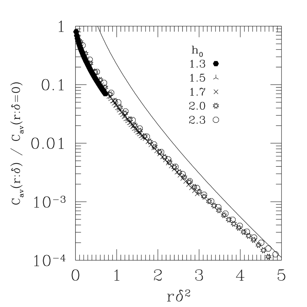
FIG. 14.: A scaling plot of the average correlation function, according to Eq. (26) with the predicted value $\nu=2$. The curve is a plot of Eq. (27) (expected to be valid for $r\delta^{2}\gg 1$) with $D=35$. Note that from Eqs. (22) and (25), one has $\xi^{-1}=\delta^{2}$ for the distribution of Eq. (7).

FIG. 15.: A scaling plot of the average of the log of the correlation function in the disordered phase according to Eq. (32). The best fit (shown) is for $\tilde{\nu}=1.1$, close to the prediction [5, 6] $\tilde{\nu}=1$. The data is an average over 10000 samples.

FIG. 16.: A scaling plot of the average of the log of the correlation function in the disordered phase according to Eq. (32), assuming the theoretical value $\tilde{\nu}=1$. The solid line is the prediction of Eq. (33), which expected to be valid at large $r$, but also works well down to $r=0$. It appears that by dividing by the correlation function at criticality, we incorporate most of the corrections to the asymptotic form in Eq. (33). Note that from Eq. (34) one has $\tilde{\xi}^{-1}=2\delta$.

We now discuss our results for the disordered phase. The scaling plot corresponding to Eq. (26) is shown in Fig. 13. The plot has $\nu=1.8$ which gave the best fit, and which agrees fairly well with the prediction $\nu=2$. A plot using $\nu=2$ works somewhat less well, presumably indicating that there are corrections to scaling for this range of lattice sizes and distances. Fig. 14 is a scaling plot using the theoretical value $\nu=2$ which also shows the asymptotic form in Eq. (27) with $D=35$. Both the data and the prediction of Eq. (27), have substantial curvature: much more than in the corresponding data for $\log C(r)$ shown in Figs. 15 and 16. Over the range of accessible values of $r\delta^{2}$, the data and the asymptotic prediction do not track each other closely, though it is possible that they would do so for larger values of $r\delta^{2}$.

The data for the log of the scaling function scales well according to Eq. (32) , though the best fit has a slightly different exponent of 1.1, see Fig. 15. Presumably this difference again indicates that there are corrections to scaling for the sizes and distances studied. Note that the data in Fig. 15 is close to a straight line but there is statistically significant curvature.

Fig. 16 tests the more stringent prediction[5, 11] for the average of $\ln C(r)$ in the limit $r\gg\tilde{\xi}$ obtained by combining Eq. (33) with the assumption that the expression for $\tilde{\xi}$ in Eq. (34) is exact for correlations of $\sigma^{z}$. One sees that it works quite well.

FIG. 17.: The distribution of the log of the correlation function for different values of $r$ at $h_{0}=3$ in the disordered phase. The data represents an average over 10000 samples for $L=64$. Both the most probable value and the width of the distribution increase with $r$ but the most probable value increases faster, see Fig. 18.

FIG. 18.: A scaling plot of the data in Fig. 17. The width of the distribution is seen to narrow with increasing $r$, as expected.

Although our best estimates of the critical exponents $\nu$ and $\tilde{\nu}$ do not quite agree with the theoretical predictions, they are fairly close to those predictions, and they differ substantially from each other, providing clear evidence that there are different correlation length exponents for the average and typical correlation functions.

Finally, in this section, we look at the distribution of $\ln C(r)$ for $r$ larger than either the average or typical correlation lengths. It is predicted[5, 6] that the distribution of $(\ln C(r))/r$ should become sharp at large $r$ in this limit. Fig. 17 shows data for the distribution of $\ln C(r)$ at $h_{0}=3$. One sees that both the peak position and the width increase with increasing $r$, but the peak position increases faster as can be seen in Fig. 18 which shows the distribution of $(\ln C(r))/r$. In Fig. 19 we test the more precise predictions[5, 11] for the mean and variance of $\ln C(r)$ given in Eqs. (37) and (38), for $h_{0}=3$. The fits give reasonable agreement with Eqs. (37) and (38), but assume a form of corrections to scaling that we have been unable to justify.

FIG. 19.: The mean and variance of the distribution of $\ln C(r)$ in the disordered phase at $h_{0}=3$ for different values of $r$. Both the mean and variance are expected be proportional to $r$ at large $r$. The lines are least squares fits of the form $a+br^{1/2}+cr$. This form is motivated by the behavior at criticality, for which the mean varies as $r^{1/2}$, and, in fact, the $r^{1/2}$ correction to scaling was effectively removed in Fig. 16 by factoring out the behavior at criticality. However it is not clear that the constant and the $r^{1/2}$ term give all the corrections to scaling in the disordered phase. The fit to the mean has $a=-0.140,b=1.145,c=1.014$, while the fit to the variance has $a=1.025,b=-1.736,c=2.029$. According to the suggestion of Fisher[11], following Shankar and Murphy[5], the leading behavior for large $r$ should be given by Eqs. (37) and (38). Noting that here, $2\delta=\ln 3\simeq 1.099$, we see that the large $r$ behavior predicted by the fits is is in rather good agreement with theory.

VI The local susceptibility

In this section we discuss the local susceptibility rather than the uniform susceptibility, because it has somewhat simpler behavior. Since it it just involves correlations on a single site, any singularity must come only from long time-correlations, whereas the uniform susceptibility involves correlations both in space and time. Our results for the uniform susceptibility away from the critical point do not scale in a simple manner, and we suspect that there are logarithmic corrections, as occurs for bulk behavior at finite temperature[6].

FIG. 20.: The distribution of the log of the local susceptibility at the critical point for different sizes obtained by the Lanczos method. The number of samples is $50000/L$, so that 50000 values for $\chi_{\rm\scriptscriptstyle loc}$ were obtained for each size.

Since it is difficult to compute the susceptibility from the fermion method, particularly with periodic boundary conditions, we have used the Lanczos diagonalization technique on the original spin Hamiltonian, Eq. (1). Of course the price we pay is that the lattices are much smaller, $L\leq 16$. The local susceptibility at $T=0$ is given by

$$\chi_{\mbox{loc}}=2\sum_{n\neq 0}{|\langle 0|\sigma^{z}_{i}|n\rangle|^{2}\over E_{n}-E_{0}}\ .$$ (87)

where $|n\rangle$ denotes a many body state of the system and $|0\rangle$ is the ground state. Because of the form of Eq. (87) we expect that the scaling of $\chi_{\mbox{loc}}$ will be very similar to that of $1/\Delta E$. This is indeed the case as seen in Fig. 20, which plots the distribution of $\ln\chi_{\mbox{loc}}$ at the critical point. The distribution broadens with system size, consistent with $z=\infty$. The data scales in the expected manner, as shown in Fig. 21, which is very similar to the corresponding plot for the energy gap in Fig. 2.

FIG. 21.: A scaling plot of the data in Fig. 20. The data scales in the same way as that for the log of the gap, see Fig. 2.

FIG. 22.: The distribution of the log of the local susceptibility in the disordered phase for different sizes obtained by the Lanczos method. The number of samples is 50000 / $L$.

Even though the range of sizes used in the Lanczos method is rather small, it is, nonetheless, capable of distinguishing $z=\infty$ scaling at the critical point from finite $z$ scaling $z$ away from the critical point. This can be seen by comparing Fig. 20 with Fig. 22, which plots the distribution of $\ln\chi_{\mbox{loc}}$ at $h_{0}=3$. In Fig. 22 the curves no longer broaden with increasing $L$ but the distributions are independent of size. The reason why there is no size dependence here but there is in the distributions of $\ln\Delta E$ in Fig. 3 is easy to understand. For $\Delta E$, we compute the probability per sample of getting a certain value, and this is proportional to $L$ in the disordered phase for small $\Delta E$, since the rare strongly correlated region can occur anywhere. We used this result in Section IV to relate the exponent in the distribution to $1/z$, see Eqs. (78) and (79). With $\chi_{\mbox{loc}}$, however, we compute the probability per site, so there is no factor of $L$ and the distribution is independent of size. This is, of course, the normal state of affairs when the lattice size is much larger than the correlation length. The slope of the straight line region in Fig. 22 agrees with the slopes in Fig. 3 and so gives the same value of z as obtained from the gap, i.e. $z\simeq 1.4$.

VII The Structure Factor

A scattering experiment measures directly the structure factor, $S(q)$, defined by

$$S(q)={1\over L}\sum_{j,l}C_{jl}e^{iq(j-l)}\ .$$ (88)

Although the distribution of individual terms in the sum is broad, it is interesting, and relevant for experiment, to ask whether there are large sample to sample fluctuations in the total. We have attempted to answer this for $q=0$, where fluctuations are expected to be largest. Fig. 23 shows a log-log plot of the average of the structure factor, $S_{\rm av}(0)$, and the standard deviation among different samples, $\delta S(0)$, plotted against $L$ at the critical point. From Eq. (20) one expects the average to vary as $L^{0.62}$ and the best fit to the numerical data has a slope of $0.64$, in reasonably good agreement. One sees that $\delta S(0)<S_{\rm av}(0)$, but the ratio of the width to the mean stays finite. One expects[11] that the distribution of $S(0)/S_{\rm av}(0)$ will be broad and independent of $L$ at large $L$, and our data is consistent with this. Note that although the equal time structure factor is not self-averaging at $T=0$, its distribution is much less broad that that of the susceptibility, which involves correlations in time. Since the structure factor at the critical point behaves like the average, rather than the typical correlation function, we expect that the behavior away from criticality will be controlled by the average correlation length.

FIG. 23.: A log-log plot of the average $q=0$ structure factor, $S_{\rm av}(0)$ and the standard deviation of the structure factor among different samples, $\delta S(0)$, for different sizes. The dashed line is a fit to the data for $S_{\rm av}(0)$ and has slope 0.64, in fairly good agreement with the theoretical expectation, obtained by integrating Eq. (20), of $\phi-1\simeq 0.32$. The solid line is just a guide to the eye. The results are obtained by averaging over 10000 samples.

VIII Conclusions

We have been able to confirm the many surprising predictions of the random transverse-Ising spin chain by applying the mapping to free fermions numerically. In particular we find very broad distributions of the energy gap and correlation functions, different exponents for the average and the typical correlation functions, and an infinite value of the dynamical exponent, $z$, at the critical point. Perhaps the most interesting new result is the scaling function for the distribution of the log of the correlation function at criticality, shown in Fig. 11, which is monotonic and has an upturn as the abscissa approaches zero. If this indicates the divergence shown in Eqs. (83) and (86), the scaling function for $(\ln C(r))/r^{1/2}$ would also give the correct exponent (though perhaps not the correct amplitude) for the average correlation function.

We have seen that the width of the distribution of the the equal time structure factor seems to be comparable to the mean at $T=0$, though presumably it becomes self-averaging at finite-$T$. By contrast, the $T=0$ susceptibility and local susceptibility have enormously broad distributions. One expects that the susceptibility will also become self averaging at finite $T$ for sufficiently large $L$, but whether the necessary size diverges as power law or exponentially as $T\to 0$ is unclear. We leave this interesting question for future study.

Crisanti and Rieger[15] have studied the random transverse Ising chain by Monte Carlo methods. They took a generalization of the bimodal distribution in Eq. (81) rather than the continuous distribution used here. From the behavior of various correlation functions they found a finite $z$ at criticality, which, however, appeared to increase with increasing randomness. We saw in section IV that corrections to finite-size scaling appear to be larger for this distribution than for the the continuous one and, furthermore, it is harder to estimate the asymptotic value of $z$ from correlation functions than from distributions. This is presumably why Crisanti and Rieger[15] did not find $z=\infty$ in their study.

After this work was largely completed we became aware of related work by Asakawa and Suzuki[16], who also used the mapping to free fermions but used the same distribution as Crisanti and Rieger. In contrast to our results, they claim that the exponents depend on the parameters in the distribution. This is lack of universality is not predicted by theory[5, 6] and a possible explanation of the discrepancy is that not all their data is in the asymptotic scaling regime, which is likely to be reached for different lattice sizes for different distributions.

It is interesting to speculate to what extent the results of the one-dimensional system go over to higher dimensions. In particular, one would like to know if $z$ is infinite at the critical point or takes a finite value for $d>1$. The results for the local susceptibility in Section VI indicate that this question can be answered even for moderately small lattice sizes provided appropriate quantities are studied. The distribution of $\ln\chi_{\mbox{loc}}$ (or the log of the gap) seems to be particularly convenient, since, for finite-$z$, data for different sizes look essentially the same, whereas for $z=\infty$ the curves get broader and broader. Of course it is still difficult to distinguish a large but finite $z$ from $z=\infty$, since the two would look the same for small sizes. With finite-$z$ scaling, the distribution has power law behavior, the power being related to $z$ as shown in Eq. (79). It is more difficult to determine $z$ by looking at the decay of correlation functions, because the asymptotic behavior is only seen at very large times or distances. Numerical studies in higher dimensions are likely to use quantum Monte Carlo simulations, because diagonalization methods, such as Lanczos, can only be carried out on very small systems and the mapping to free fermions only works in one-dimension. Unfortunately, there is an additional difficulty with quantum Monte Carlo, not present here, because one generally works in imaginary time, which has to be discretized. The quantum problem is recovered when the number of time slices tends to infinity, but in practice one can only simulate a finite number. It is unclear whether the extrapolation to an infinite number of time slices will pose serious difficulties for the study of Griffiths singularities and critical phenomena in higher dimensional systems.

We have seen that the disordered Griffiths phase can be conveniently parameterized by a continuously varying dynamical exponent $z$. This characterizes the distribution of the energy gap or local susceptibility for lattice sizes which satisfy the condition, $L\gg\xi$. By contrast, at the critical point, the correlation length diverges so the value of $z$ at criticality involves physics in the opposite limit, $L\ll\xi$. It is therefore possible that the limit of $z(\delta)$ for $\delta\to 0$ is not equal to the value of $z$ at criticality. Both these quantities are infinite for the transverse field Ising chain, but it would be interesting to see if there is a difference between them in higher dimensions. We expect that the results and method of analysis presented here will provide guidance for such a study.

- [1] By a quantum phase transition we mean a transition that occurs at , induced by varying some parameter other than the temperature. For the model in Eq. (1), this parameter will be the average value of the transverse field divided by the average interaction, in Eq. (7). Alternatively, we can parameterize the model by defined in Eq. (12), which is related to by Eq. (8).
- [2] R. B. Griffiths, Phys. Rev. Lett. 23. 17 (1969).
- [3] A. B. Harris, Phys. Rev. B 12, 203 (1975).
- [4] B. M. McCoy and T. T. Wu, Phys. Rev. B 176, 631 (1968); 188, 982 (1969).
- [5] R. Shankar and G. Murphy, Phys. Rev. B 36, 536 (1987).
- [6] D. S. Fisher, Phys. Rev. Lett. 69, 534 (1992); Phys. Rev. B 51, 6411 (1995).
- [7] E. Lieb, T. Schultz and D. Mattis, Ann. Phys. (NY) 16, 407 (1961).
- [8] S. Katsura, Phys. Rev. 127, 1508 (1962).
- [9] P. Pfeuty, Ann. Phys. (NY) 27, 79 (1970); Thèse, Université de Paris, (1970).
- [10] We use the term “Griffiths phase” to denote the range of values of where Griffiths singularities occur at . In general, this covers that part of the disordered phase where some of the are smaller than some of the , and also that part of the ordered phase where some of the are smaller than some of the . For the distribution in Eq. (7), which has no lower bound on the or , the Griffiths phase occurs for all . In this paper we do not consider the ordered phase ().
- [11] D. S. Fisher (private communication).
- [12] “Numerical Recipes”, by W. H. Press, B. P. Flannery, S. A. Teukolsky and W. T. Vetterling, 2nd Edition, Cambridge University Press, (Cambridge, London) (1992).
- [13] For the random problem, as well as for the pure problem, one eigenvalue hits zero as (or equivalently ) is varied. For the pure system this occurs precisely at the bulk critical point, but, for the random case, the point where the eigenvalue vanishes depends on the particular realization of the disorder, the values for different samples being scattered around the critical point. Hence, for the pure system, one knows to choose Eq. (57) or (58) for depending on whether the system is in the disordered or ordered phase, but there is no such simple criterion for the random case. We therefore need to explicitly check whether the number of bare particles, , is even or odd in the state with no quasi-particles.
- [14] M. J. Thill and D. A. Huse, Physica A, 15 1995.
- [15] A. Crisanti and H. Rieger, J. Stat. Phys. 77, 1087 (1994).
- [16] H. Asakawa and M. Suzuki (unpublished).