Theory of Cylindrical Tubules and Helical Ribbons of Chiral Lipid Membranes

Abstract

We present a general theory for the equilibrium structure of cylindrical tubules and helical ribbons of chiral lipid membranes. This theory is based on a continuum elastic free energy that permits variations in the direction of molecular tilt and in the curvature of the membrane. The theory shows that the formation of tubules and helical ribbons is driven by the chirality of the membrane. Tubules have a first-order transition from a uniform state to a helically modulated state, with periodic stripes in the tilt direction and ripples in the curvature. Helical ribbons can be stable structures, or they can be unstable intermediate states in the formation of tubules.

I Introduction

Chiral amphiphilic molecules can self-assemble into microstructures with a variety of morphologies. Two of the most interesting morphologies, both for basic research and for technological applications, are cylindrical tubules and helical ribbons [1, 2, 3]. Tubules are bilayer or multilayer membranes of amphiphilic molecules wrapped in a cylinder, as shown in Fig. 1 [4]. They are observed in a variety of systems, including diacetylenic lipids [1, 5], bile [6], surfactants [7], and glutamates [8]. In diacetylenic lipid systems, the tubule diameter is typically 0.5 $\mu$m and the tubule length is typically 50–200 $\mu$m; in other systems, the tubule dimensions are typically several times larger [6]. In most of these systems, tubules exhibit a helical “barber-pole” pattern on the surface of the cylinder. Helical ribbons are similar microstructures, consisting of long twisted strips of membranes with their edges exposed to the solvent, as shown in Fig. 2 [9]. In some cases, helical ribbons are unstable precursors to the formation of tubules; in other cases, helical ribbons appear to be stable. Cylindrical tubules have been studied extensively for use in several technological applications, such as electroactive composites and controlled-release systems [2]. Helical ribbons have not been used in technological applications, but they have also been studied extensively as part of an effort to rationally control the self-assembly of tubules.

There have been three general approaches to the theory of tubules and helical ribbons. First, de Gennes argued that a membrane of chiral molecules in any tilted phase must develop a spontaneous electrostatic polarization [10]. This polarization can induce a narrow strip of membrane to buckle into a cylinder. The original theory of de Gennes described buckling along the long axis of a cylinder, but a straightforward modification describes helical winding due to electrostatic interactions. This theoretical approach predicts that adding of electrolytes to the solvent should increase the radius of the resulting tubules, because the electrostatic interaction would be screened by electrolytes in solution. However, experiments have shown that electrolytes in solution do not affect the formation or radius of tubules [11], except for the particular case of tubules composed of amphiphiles with charged head groups [12]. Thus, electrostatic interaction is very probably not a dominant factor in tubule formation.

As an alternative theoretical approach, Lubensky and Prost derived a general phase diagram for membranes with in-plane orientational order, which predicts cylinders as well as spheres, flat disks, and tori [13]. Within the cylindrical phase, the cylinder radius and length are determined by a competition between the curvature energy and the edge energy. One important prediction of this theory is the scaling $r\propto\ell^{1/2}$ between the tubule radius $r$ and the tubule length $\ell$. However, experiments have found no correlation between $r$ and $\ell$. Rather, in a typical sample of tubules, $r$ is quite monodisperse while $\ell$ varies widely [14]. Thus, the competition between curvature energy and edge energy is also not a dominant factor in tubule formation.

A third approach, which is consistent with the experimental results on lipid tubules, is based on the chiral packing of the molecules in a membrane. Helfrich and Prost have shown that a chiral membrane in a tilted phase will form a cylinder because of an intrinsic bending force due to chirality [15]. This bending force arises because long chiral molecules do not pack parallel to their neighbors, but rather at a nonzero twist angle with respect to their neighbors. If the molecules lie in bilayers, and are tilted with respect to the local layer normal, the favored twist from neighbor to neighbor leads the whole membrane to twist into a cylinder.

Several investigators have generalized the original Helfrich-Prost concept of an intrinsic chiral bending force in different ways. Ou-Yang and Liu have developed a version of this theory based on an analogy with cholesteric liquid crystals [16]. Chappell and Yager have developed an analogous theory in which the direction of one-dimensional chains of molecules, rather than the direction of molecular tilt, defines a vector order parameter within the membrane [17]. Nelson and Powers have used the renormalization group to calculate the effects of thermal fluctuations on tubules [18]. This calculation predicts an anomalous scaling of the tubule radius as a function of the strength of the chiral interaction. Chung et al. have considered the full elastic anisotropy of a membrane, and have related the pitch angle of tubules to a ratio of membrane elastic constants [6]. They have also made predictions for the kinetic evolution of helical ribbons into tubules.

In our earlier paper, we generalized the Helfrich-Prost concept in another way [19]. In that theory, we began with a three-dimensional (3D) liquid-crystal free energy and applied it to the case of chiral molecules in a membrane. We showed that the chiral term in this free energy has two simultaneous effects: it leads the membrane to twist into a cylinder, and it induces a variation in the direction of the molecular tilt on the cylinder. Through this calculation, we predicted that tubules can form periodic modulated structures characterized by helical stripes in the tilt direction winding around the cylinders, as shown in Fig. 3. These stripes are analogous to the stripes seen in thin films of chiral smectic liquid crystals [20, 21, 22], but in a cylindrical rather than a planar geometry. We argued that these stripes correspond to the helical substructure that is often observed on tubules.

In this paper, we further extend this theoretical approach to provide a more unified and systematic model of tubules and helical ribbons. First, we combine our earlier theory with the Chung theory to obtain a theory of tubules with both elastic anisotropy and tilt modulation. We derive explicit expressions for the average direction of the tilt and for the direction of the modulation, in terms of the elastic coefficients, and we show that these directions are different. Next, we show that the same theory can also be applied to helical ribbons. This theory shows that helical ribbons can be stable microstructures for a certain range of parameters; they are not necessarily intermediate states in the formation of tubules. Finally, we investigate the effects of the striped tilt modulation on the detailed shape of tubules. Based on recent models of lipid bilayers [23, 24], we expect a modulation in the tilt to induce a modulation in the curvature. We predict the curvature modulation illustrated in Fig. 4, which resembles the $P_{\beta^{\prime}}$ rippled phases of lyotropic liquid crystals [25, 26].

The plan of this paper is as follows. In Sec. II, we construct a free energy for tubules and helical ribbons, which includes elastic anisotropy and includes the possibility of tilt modulation. In Sec. III, we use this free energy to predict the radius and tilt direction for tubules with uniform tilt. The results of that section are in exact agreement with the theory of Chung et al. In Sec. IV, we consider tubules with a modulation in the tilt. We propose an explicit ansatz for that modulation, and then minimize the free energy over the parameters in that ansatz. We find that there is a first-order transition from uniform to modulated tubules. In Sec. V, we apply the same theory to helical ribbons. The theory predicts the range of parameters in which helical ribbons are stable. In Sec. VI, we investigate ripples in the curvature of tubules and helical ribbons. We derive an explicit expression for the ripple shape that corresponds to our ansatz for the tilt modulation. Finally, in Sec. VII, we discuss these theoretical predictions and compare them with experimental results.

II Free Energy

In this section, we construct a free energy for tubules and helical ribbons. In this free energy, we suppose that the membrane is in a fluid phase, which may have hexatic bond-orientational order but does not have crystalline positional order. This assumption is based on the theoretical argument of Nelson and Peliti, who showed that a flexible membrane cannot have crystalline positional order in thermal equilibrium at nonzero temperature, because thermal fluctuations induce dislocations, which destroy this order on long length scales [27]. This assumption is also supported by two types of experimental evidence. First, Treanor and Pace found a distinct fluid character in nuclear magnetic resonance and electron spin resonance experiments on tubules [28]. Second, Brandow et al. found that tubule membranes can flow to seal up cuts in the membrane from an atomic force microscope tip [29]. This flow indicates that the membrane has no shear modulus [30]. Further information on the membrane phase comes from Thomas et al., who found long positional correlation lengths of 0.068 to 0.135 $\mu$m in synchrotron x-ray scattering studies of tubules [31]. Taken together, all of these experimental results suggest that tubule membranes are in a highly correlated hexatic phase.

In this paper, we do not attempt to derive the free energy from a 3D liquid-crystal free energy, as in our earlier paper [19]. Rather, we use a 2D differential-geometry notation, which is more general. In this notation, the curvature of a membrane is described by the curvature tensor $K_{ab}$. The orientation of the molecular tilt is represented by the unit vector $\vec{m}$. As shown in Fig. 5, $\vec{m}$ is the projection of the molecular director $\vec{n}$ into the local tangent plane, normalized to unit magnitude.

A membrane may consist of a single domain, in which the curvature $K_{ab}$ is low and the tilt direction $\vec{m}$ varies smoothly. Alternatively, a membrane may consist of many internal domains separated by domain walls. Domain walls are sharp boundaries between domains. Across a narrow domain wall, $\vec{m}$ jumps abruptly and $K_{ab}$ may become high. Here, we will consider the free energy of domains and domain walls separately.

First, we consider a domain of low curvature and smoothly varying tilt. Within a domain of a membrane, the free energy can be written as

$$F=\int dA\biggl{[} \frac{1}{2}\kappa\left(K^{a}_{a}\right)^{2}+\frac{1}{2}\kappa^{\prime}m^{a}m^{b}K_{ac}K^{c}_{b}$$ (4)

$$+\lambda_{\rm HP}m^{a}m^{c}K^{b}_{a}\sqrt{g}\epsilon_{bc}$$

$$-\lambda_{\rm LS}\sqrt{g}\epsilon_{ab}D^{a}m^{b}-\gamma K^{a}_{a}D_{b}m^{b}$$

$$+\frac{1}{2}c\left[\left(\sqrt{g}\epsilon_{ab}D^{a}m^{b}\right)^{2}+\left(D_{a}m^{a}\right)^{2}\right]\biggr{]}.$$

Here, the surface area element is $dA=\sqrt{g}d^{2}x$, $\epsilon_{ab}$ is the antisymmetric symbol, and $D_{a}$ is the covariant derivative within the membrane. Throughout this work, we shall imply summation over repeated indices, such as $a$ in the first term above. The first term of $F$ is the standard Helfrich bending energy of the membrane [32]. The coefficient $\kappa$ is the isotropic rigidity. The second term represents the anisotropy of the rigidity. The coefficient $\kappa^{\prime}$ is the difference between the energy required to bend the membrane parallel to the tilt $\vec{m}$ and the energy required to bend it perpendicular to $\vec{m}$. In general, $\kappa^{\prime}$ can be either positive or negative. The third term, introduced by Helfrich and Prost [15], is a chiral term that favors curvature in a direction $45^{\circ}$ from $\vec{m}$. The coefficient $\lambda_{{\rm HP}}$ is a measure of the magnitude of the chiral interaction between the molecules in the membrane. The fourth term is another chiral term, which favors a bend in $\vec{m}$. This term was introduced by Langer and Sethna in the context of flat films of chiral liquid crystals [20]. The coefficient $\lambda_{{\rm LS}}$ should have the same magnitude as $\lambda_{{\rm HP}}$; both coefficients are comparable to $Kq$ in the notation of our earlier paper [19]. However, there is no symmetry reason why $\lambda_{{\rm LS}}$ and $\lambda_{{\rm HP}}$ must be equal. The fifth term, with coefficient $\gamma$, is the coupling between curvature of the membrane and splay of $\vec{m}$. It can be understood in two equivalent ways: (a) the curvature of the membrane breaks the symmetry between the two monolayers of a bilayer and hence induces a splay in $\vec{m}$, or (b) a splay in $\vec{m}$ induces a curvature of the membrane to keep the molecules more nearly parallel in three dimensions. This term is equivalent to terms that have been considered in the Lubensky-MacKintosh theory of $P_{\beta^{\prime}}$ rippled phases [23, 24]. The final pair of terms is the 2D Frank free energy for variations in $\vec{m}$. It provides an energy penalty for tilt variations, and hence limits those variations. The coefficient $c$ is a single Frank constant.

We now consider a domain wall between two domains. Across a domain wall, the tilt direction $\vec{m}$ changes abruptly. The curvature $K_{ab}$ may also become large, giving a “crease” in the membrane. For those reasons, different parts of the molecules come into contact at a domain walls than inside the domains. A domain wall therefore costs an energy $\epsilon_{W}$ per unit length. The domain-wall energy cannot be derived from the free energy (4) within a domain; rather, it is an additional parameter that describes narrow walls where that free energy does not apply. For any morphology that includes domain walls, with a total wall length $L_{W}$, the total free energy is $F_{{\rm tot}}=F+\epsilon_{W}L_{W}$.

In the free energy (4), the term $\lambda_{{\rm LS}}\sqrt{g}\epsilon_{ab}D^{a}m^{b}$ is a total derivative. If the curvature is constant, as in a perfect cylinder, the term $\gamma K_{a}^{a}D_{b}m^{b}$ is also a total derivative. One might think that these terms integrate to constants and hence do not affect the morphology of a membrane. However, these terms are significant if the membrane consists of internal domains separated by domain walls, because they then become line integrals along the domain walls. Indeed, these terms favor the formation of a series of domains separated by domain walls, because they can contribute a negative free energy for each domain. Thus, in the rest of this paper, we will retain these terms, and we will explicitly compare their negative contribution to the free energy with the energy cost of the domain walls.

The free energy (4) does not contain an exhaustive list of all the terms permitted by symmetry; other terms are also possible. For example, the term $(m^{a}m^{b}K_{ab})^{2}$ would give an additional elastic anisotropy, which has been considered by Chung et al. [6]. The combination $(\sqrt{g}\epsilon_{ab}D^{a}m^{b})^{2}-(D_{b}m^{b})^{2}$ would give a difference in the Frank constants for bend and splay. Rather, this free energy is only intended to include the terms that generate distinct physical effects, while the omitted terms give higher-order details of the structure.

If the membrane forms a perfect cylinder with radius $r$, the free energy (4) simplifies greatly. In the standard cylindrical coordinates $(\theta,z)$, the curvature tensor becomes

$$K=\left(\begin{array}[]{cc}-1/r&0\\ 0&0\end{array}\right).$$ (5)

The tilt director field can be written as $\vec{m}(\theta,z)=(\cos\phi,\sin\phi)$. As shown in Fig. 5, $\phi(\theta,z)$ is the angle in the local tangent plane between the tilt direction and the equator of the cylinder. The free energy then becomes

$$F=\int dA\biggl{[} \frac{1}{2}\kappa\left(\frac{1}{r}\right)^{2}+\frac{1}{2}\kappa^{\prime}\left(\frac{1}{r}\right)^{2}\cos^{2}\phi$$ (9)

$$-\lambda_{\rm HP}\left(\frac{1}{r}\right)\sin\phi\cos\phi$$

$$-\lambda_{\rm LS}\vec{\nabla}\times\vec{m}+\gamma\left(\frac{1}{r}\right)\vec{\nabla}\cdot\vec{m}$$

$$+\frac{1}{2}c\left[\left(\vec{\nabla}\times\vec{m}\right)^{2}+\left(\vec{\nabla}\cdot\vec{m}\right)^{2}\right]\biggr{]},$$

where $dA=rd\theta dz$,

$$\vec{\nabla}\times\vec{m}=\frac{1}{r}\partial_{\theta}\sin\phi-\partial_{z}\cos\phi,$$ (10)

and

$$\vec{\nabla}\cdot\vec{m}=\frac{1}{r}\partial_{\theta}\cos\phi+\partial_{z}\sin\phi.$$ (11)

Note that the 2D cross product defined by Eq. (10) is a scalar. This form of the free energy is generally more convenient to work with than the more general form (4). The interpretation of these terms is exactly as discussed above. In the following sections, we will use this free energy to investigate the structure of tubules and helical ribbons.

III Tubules with Uniform Tilt

As a first step in understanding the implications of the free energy (4), we consider tubules with a uniform tilt direction $\vec{m}$. This model of uniform tubules is equivalent to the model of Chung et al. [6]. We present it here in order to review their results in our notation.

Suppose that a tubule of radius $r$ has a uniform tilt $\vec{m}=(\cos\phi_{0},\sin\phi_{0})$, at an angle $\phi_{0}$ away from the equator, as shown in Fig. 6. The entire tubule is a single domain, with no domain walls. In terms of $r$ and $\phi_{0}$, the free energy per unit area is

$$\frac{F}{A}= \frac{1}{2}\kappa\left(\frac{1}{r}\right)^{2}+\frac{1}{2}\kappa^{\prime}\left(\frac{1}{r}\right)^{2}\cos^{2}\phi_{0}$$ (13)

$$-\lambda_{\rm HP}\left(\frac{1}{r}\right)\sin\phi_{0}\cos\phi_{0}.$$

Minimizing this expression over $r$ and $\phi_{0}$ simultaneously, we obtain

$$r=\frac{\kappa^{1/4}\left(\kappa+\kappa^{\prime}\right)^{1/4}\left[\kappa^{1/2}+\left(\kappa+\kappa^{\prime}\right)^{1/2}\right]}{\lambda_{{\rm HP}}}$$ (14)

and

$$\phi_{0}=\arctan\left[\left(\frac{\kappa+\kappa^{\prime}}{\kappa}\right)^{1/4}\right].$$ (15)

These results lead to two important conclusions. First, the tubule radius $r$ scales inversely with the chirality parameter $\lambda_{{\rm HP}}$. In a nonchiral membrane, where $\lambda_{{\rm HP}}\rightarrow 0$, the radius $r\rightarrow\infty$. The coefficient of $1/\lambda_{{\rm HP}}$ is a combination of the elastic constants $\kappa$ and $\kappa^{\prime}$. Second, the tilt direction $\phi_{0}$ is determined by the ratio of the energy cost $\kappa+\kappa^{\prime}$ for bend parallel to the tilt direction over the energy cost $\kappa$ for bend perpendicular to the tilt direction. In an isotropic membrane, where $\kappa^{\prime}=0$, we obtain $\phi_{0}=45^{\circ}$. In an anisotropic membrane, $\kappa^{\prime}$ may be positive or negative, and hence $\phi_{0}$ may be greater or less than $45^{\circ}$.

Chung et al. [6] originally derived Eq. (15) in order to analyze experimental data on tubules in bile. In experiments on bile systems, they found two types of tubules. Both types of tubules show clear helical markings, but the direction of these markings are different: $53.7^{\circ}$ from the equator in one type of tubule and $11.1^{\circ}$ from the equator in the other. Chung et al. assumed that these helical markings are aligned with the molecular tilt, so that $\phi_{0}=53.7^{\circ}$ and $11.1^{\circ}$ in the two types of tubules. They then used Eq. (15) to determine the values of $(\kappa+\kappa^{\prime})/\kappa$ that correspond to these values of $\phi_{0}$. The resulting values are $(\kappa+\kappa^{\prime})/\kappa=3.4$ and 0.0015, respectively. The ratio of 3.4 is quite reasonable, but the ratio of 0.0015 is surprising. It seems unlikely that a bend in the membrane perpendicular to the tilt direction would cost almost 1000 times more energy than a bend parallel to the tilt direction. For that reason, we must re-examine the assumption that helical markings are aligned with the molecular tilt. In the following section, we propose an alternative interpretation of the helical markings, which can explain this anomaly.

IV Tubules with Tilt Modulation

In this section, we relax the assumption that the tilt direction $\vec{m}$ is uniform everywhere on a tubule. Instead, we allow $\vec{m}$ to vary as a function of the cylindrical coordinates $\theta$ and $z$, with $\vec{m}(\theta,z)=(\cos\phi(\theta,z),\sin\phi(\theta,z))$. We show that the ground state of the tubule can have a periodic helical modulation of $\vec{m}$.

As a specific ansatz, we suppose that there are $n$ distinct stripes in the tilt direction. In the terminology of Sec. II, each stripe is a single domain of the membrane. The stripes are separated by $n$ distinct domain walls. The stripes and domain walls run around the cylinder helically, as shown in Fig. 3. We further suppose that the tilt direction $\phi$ varies linearly across each stripe. Across each domain wall, $\phi$ changes sharply, almost discontinuously on the scale of the stripes. The direction of the stripes and the domain walls is defined by the angle $\omega$ with respect to the equator of the cylinder, illustrated in Fig. 7. Let $\theta^{\prime}$ be the coordinate running along the $\omega$ direction,

$$\theta^{\prime}\equiv\theta+\frac{z}{r}\tan\omega.$$ (16)

In terms of this coordinate, our ansatz for the tilt direction $\phi$ can be written as

$$\phi(\theta,z)=\phi_{0}+\frac{n\Delta\phi}{2\pi}\left(\theta^{\prime}\bmod\frac{2\pi}{n}\right),$$ (17)

where $\theta^{\prime}\bmod 2\pi/n$ runs from $-\pi/n$ to $\pi/n$. This ansatz has the sawtooth form shown in Fig. 8. It oscillates about the average value $\phi_{0}$ with the amplitude $\Delta\phi$. Thus, our ansatz has five variational parameters: the radius $r$, the average tilt direction $\phi_{0}$, the amplitude of the tilt variation $\Delta\phi$, the stripe direction $\omega$, and the number of distinct stripes $n$. In terms of these parameters, the stripe width is

$$L=\left(\frac{2\pi}{n}\right)r\cos\omega.$$ (18)

We must now express the free energy (9) in terms of the five variational parameters. To simplify the algebra, we suppose that $\Delta\phi\ll 1$; i. e., there is only a small variation in the tilt direction. We will discuss corrections to this approximation at the end of this section. The curl and divergence of the tilt then become

$$\vec{\nabla}\times\vec{m}=\frac{n\Delta\phi\cos\left(\phi_{0}-\omega\right)}{2\pi r\cos\omega}$$ (19)

and

$$\vec{\nabla}\cdot\vec{m}=-\frac{n\Delta\phi\sin\left(\phi_{0}-\omega\right)}{2\pi r\cos\omega}.$$ (20)

With these expressions, it is straightforward to work out the gradient terms in Eq. (9).

The terms $\frac{1}{2}\kappa^{\prime}r^{-2}\cos^{2}\phi-\lambda_{{\rm HP}}r^{-1}\sin\phi\cos\phi$ require special attention. This combination of terms favors a particular orientation $\phi_{0}$ of the tilt direction with respect to the equator of the cylinder. Because it gives an energy penalty for variations in the tilt away from the optimum direction, it depends on $\Delta\phi$ as well as on $\phi_{0}$ and $r$. We expand this combination as a power series in $(\phi-\phi_{0})$, then average it over the cylinder (i. e., average it over the coordinate $\theta^{\prime}$). The result can be written as $\frac{1}{2}\kappa^{\prime}r^{-2}\cos^{2}\phi_{0}-\lambda_{{\rm HP}}r^{-1}\sin\phi_{0}\cos\phi_{0}+\frac{1}{2}\nu(\Delta\phi)^{2}$, where

$$\nu=\frac{1}{6}\left[\left(\frac{\kappa^{\prime}}{2r^{2}}\right)^{2}+\left(\frac{\lambda_{{\rm HP}}}{r}\right)^{2}\right]^{1/2}.$$ (21)

The term $\frac{1}{2}\nu(\Delta\phi)^{2}$ gives the energy penalty for variations of $\phi$ away from $\phi_{0}$.

The domain-wall energy also requires special attention. As noted in Sec. II, the continuum free energy of Eqs. (4) and (9) does not describe the narrow regions inside the domain walls. Rather, we must explicitly add the domain-wall energy $\epsilon_{W}$ per unit length. In principle, $\epsilon_{W}$ can depend on $\phi_{0}$, $\Delta\phi$, and $\omega$. In this paper, we will neglect that possible variation and treat $\epsilon_{W}$ as a constant. In an area $A$ of the membrane, the total length of all the domain walls is $L_{W}=A/L$. The domain-wall energy per unit area of membrane therefore becomes

$$\frac{\epsilon_{W}L_{W}}{A}=\frac{\epsilon_{W}n}{2\pi r\cos\omega}.$$ (22)

Putting all the pieces together, the total free energy per unit area for our ansatz now becomes

$$\frac{F_{\rm tot}}{A}= \frac{1}{2}\kappa\left(\frac{1}{r}\right)^{2}+\frac{1}{2}\kappa^{\prime}\left(\frac{1}{r}\right)^{2}\cos^{2}\phi_{0}$$ (26)

$$-\lambda_{\rm HP}\left(\frac{1}{r}\right)\sin\phi_{0}\cos\phi_{0}+\frac{1}{2}\nu(\Delta\phi)^{2}$$

$$-\lambda_{\rm LS}\frac{n\Delta\phi\cos\left(\phi_{0}-\omega\right)}{2\pi r\cos\omega}-\frac{\gamma}{r}\frac{n\Delta\phi\sin\left(\phi_{0}-\omega\right)}{2\pi r\cos\omega}$$

$$+\frac{1}{2}c\left(\frac{n\Delta\phi}{2\pi r\cos\omega}\right)^{2}+\frac{\epsilon_{W}n}{2\pi r\cos\omega}.$$

This expression must be minimized over the five variational parameters $r$, $\phi_{0}$, $\Delta\phi$, $\omega$, and $n$.

To do this minimization, we will make an approximation: We will treat $n$ as a continuous variable rather than as an integer. This should be a good approximation for $n\gg 1$, although not for $n\approx 1$. We will discuss corrections to this approximation, as well as the previous one, at the end of this section. After making this approximation, it is convenient to change variables from $n$ to $L=(2\pi r\cos\omega)/n$. We also change variables from $\omega$ to $\delta=\phi_{0}-\omega$. The variable $L$ is the stripe width, as noted above, and $\delta$ is the difference between the average tilt direction and the stripe direction. In terms of these variables, the free energy (26) simplifies to

$$\frac{F_{\rm tot}}{A}= \frac{1}{2}\kappa\left(\frac{1}{r}\right)^{2}+\frac{1}{2}\kappa^{\prime}\left(\frac{1}{r}\right)^{2}\cos^{2}\phi_{0}$$ (30)

$$-\lambda_{\rm HP}\left(\frac{1}{r}\right)\sin\phi_{0}\cos\phi_{0}+\frac{1}{2}\nu(\Delta\phi)^{2}$$

$$-\lambda_{\rm LS}\frac{\Delta\phi\cos\delta}{L}-\frac{\gamma}{r}\frac{\Delta\phi\sin\delta}{L}$$

$$+\frac{1}{2}c\left(\frac{\Delta\phi}{L}\right)^{2}+\frac{\epsilon_{W}}{L}.$$

This expression for the free energy must be minimized over the five variational parameters $r$, $\phi_{0}$, $\Delta\phi$, $\delta$, and $L$.

As a first step, we minimize the free energy over the angle $\delta$. We obtain

$$\tan\delta=\frac{\gamma}{r\lambda_{{\rm LS}}}.$$ (31)

This expression is equivalent to the corresponding result in our earlier paper [19]. This result is important because the angle $\delta$ gives the difference between the stripe direction $\omega$ and the average tilt direction $\phi_{0}$. Because these two directions differ by an angle $\delta$, we can explain the anomaly mentioned at the end of Sec. III. Recall that the experiments of Chung et al. [6] found one type of tubules with helical markings at an angle of $11.1^{\circ}$ from the equator. If these helical markings indicate the average tilt direction $\phi_{0}$, then the ratio of rigidities $(\kappa+\kappa^{\prime})/\kappa$ must be 0.0015, an anomalously low value. However, if the helical markings indicate the stripe direction, then this result for $(\kappa+\kappa^{\prime})/\kappa$ does not hold. That ratio could be closer to 1, and the angle $\phi_{0}$ could be closer to $45^{\circ}$, while the stripe direction is $11.1^{\circ}$. Thus, our interpretation is that those experiments were measuring the stripe direction, not the average tilt direction.

One might think that $\delta$ would be very small because $\tan\delta$ scales as $1/r$ and $r$ is large. However, in Sec. III we showed that $r$ scales as $\kappa/\lambda_{{\rm HP}}$. For that reason, $\tan\delta$ scales as $(\gamma\lambda_{{\rm HP}})/(\lambda_{{\rm LS}}\kappa)$. We have already argued that the chiral coefficients $\lambda_{{\rm HP}}$ and $\lambda_{{\rm LS}}$ should have roughly the same magnitude. Hence, we obtain

$$\tan\delta\sim\frac{\gamma}{\kappa}.$$ (32)

This ratio can be large or small.

For the next step in the calculation, we substitute Eq. (31) for $\delta$ back into Eq. (30) for the free energy, to obtain

$$\frac{F_{\rm tot}}{A}= \frac{1}{2}\kappa\left(\frac{1}{r}\right)^{2}+\frac{1}{2}\kappa^{\prime}\left(\frac{1}{r}\right)^{2}\cos^{2}\phi_{0}$$ (36)

$$-\lambda_{\rm HP}\left(\frac{1}{r}\right)\sin\phi_{0}\cos\phi_{0}+\frac{1}{2}\nu(\Delta\phi)^{2}$$

$$-\left[\lambda_{\rm LS}^{2}+\left(\frac{\gamma}{r}\right)^{2}\right]^{1/2}\frac{\Delta\phi}{L}$$

$$+\frac{1}{2}c\left(\frac{\Delta\phi}{L}\right)^{2}+\frac{\epsilon_{W}}{L}.$$

Minimizing this expression over the stripe width $L$ gives

$$L=\frac{c(\Delta\phi)^{2}}{\left[\lambda_{{\rm LS}}^{2}+(\gamma/r)^{2}\right]^{1/2}\Delta\phi-\epsilon_{W}}$$ (37)

if this denominator is positive, or $L\rightarrow\infty$ otherwise. This expression for $L$ is the same result that one would expect from studies of stripes in flat films [20, 21, 22]. It is equivalent to the result for stripes in tubules in our earlier paper [19], except that the dependence on $\Delta\phi$ was not considered there. This expression shows that the $\lambda_{{\rm LS}}$ and $\gamma/r$ terms in the free energy both tend to induce stripes with a narrow width. If the energy gain from these terms, added in quadrature, exceeds the energy cost $\epsilon_{W}$ of a domain wall, then stripes will form; otherwise they will not form. If stripes do form, their width depends on the competition between the Frank free energy proportional to $c$, which resists variation in $\phi$, and the $\lambda_{{\rm LS}}$ and $\gamma/r$ terms.

We now insert Eq. (37) for $L$ back into Eq. (36) for the free energy. The result is

$$\frac{F_{\rm tot}}{A}= \frac{1}{2}\kappa\left(\frac{1}{r}\right)^{2}+\frac{1}{2}\kappa^{\prime}\left(\frac{1}{r}\right)^{2}\cos^{2}\phi_{0}$$ (40)

$$-\lambda_{\rm HP}\left(\frac{1}{r}\right)\sin\phi_{0}\cos\phi_{0}+\frac{1}{2}\nu(\Delta\phi)^{2}$$

$$-\frac{1}{2c}\left[\left[\lambda_{\rm LS}^{2}+\left(\frac{\gamma}{r}\right)^{2}\right]^{1/2}-\frac{\epsilon_{W}}{\Delta\phi}\right]^{2}.$$

if the quantity in brackets in the last term is positive. If not, then the last term is zero. Because only the last two terms in the free energy depend on $\Delta\phi$, we will call them $F_{{\rm stripe}}(\Delta\phi)/A$. We must now minimize $F_{{\rm stripe}}$ over $\Delta\phi$. This minimization cannot be done analytically, but it can be done graphically. In Fig. 9, we plot $F_{{\rm stripe}}$ as a function of $\Delta\phi$ for a sequence of values of $\nu$. The parameter $\nu$, defined in Eq. (21), gives the energy penalty for variations of $\phi$ away from $\phi_{0}$. For large $\nu$, the only minimum of $F_{{\rm stripe}}$ is for $\Delta\phi=0$. That is reasonable, because a large value of $\nu$ suppresses all variations in $\phi$. As $\nu$ decreases, $F_{{\rm stripe}}$ develops a local minimum for $\Delta\phi\neq 0$. At a critical value $\nu_{c}$, there is a first-order transition from $\Delta\phi=0$ to $\Delta\phi=\Delta\phi_{c}$. For $\nu<\nu_{c}$, the minimum at $\Delta\phi\neq 0$ becomes the absolute minimum of the free energy. To calculate $\nu_{c}$ and $\Delta\phi_{c}$, we set $F_{{\rm stripe}}=0$ and $\partial F_{{\rm stripe}}/\partial(\Delta\phi)=0$. The result is

$$\nu_{c}=\frac{1}{16c\epsilon_{W}^{2}}\left[\lambda_{{\rm LS}}^{2}+\left(\frac{\gamma}{r}\right)^{2}\right]^{2}$$ (41)

and

$$\Delta\phi_{c}=\frac{2\epsilon_{W}}{\left[\lambda_{{\rm LS}}^{2}+(\gamma/r)^{2}\right]^{1/2}}.$$ (42)

The corresponding value of the stripe width is

$$L_{c}=\frac{4c\epsilon_{W}}{\lambda_{{\rm LS}}^{2}+(\gamma/r)^{2}},$$ (43)

and hence the gradient in the tilt direction $\phi$ is

$$\frac{\Delta\phi_{c}}{L_{c}}=\frac{\left[\lambda_{{\rm LS}}^{2}+(\gamma/r)^{2}\right]^{1/2}}{2c}.$$ (44)

In summary, for $\nu>\nu_{c}$ the tubules are uniform, with no tilt modulation. In that case, we have $\Delta\phi=0$, $L\rightarrow\infty$, and $F_{{\rm stripe}}=0$. At $\nu=\nu_{c}$, there is a first-order transition from the uniform state to a modulated state with $\Delta\phi=\Delta\phi_{c}$ and $L=L_{c}$. At this point, $F_{{\rm stripe}}$ is still zero. For $\nu<\nu_{c}$, the tubules remain in the modulated state. As $\nu$ decreases, $\Delta\phi$ and $L$ both grow larger and $F_{{\rm stripe}}$ becomes negative. It is not possible to derive a general analytic expression for $\Delta\phi$ and $L$ in the modulated state. However, a good estimate would be $\Delta\phi\approx\Delta\phi_{c}$ and $L\approx L_{c}$.

We must now minimize the free energy (40) over the radius $r$ and the average tilt direction $\phi_{0}$, which are the remaining variational parameters. For $\nu\geq\nu_{c}$, we have $F_{{\rm stripe}}=0$, and hence the total free energy is

$$\frac{F_{\rm tot}}{A}= \frac{1}{2}\kappa\left(\frac{1}{r}\right)^{2}+\frac{1}{2}\kappa^{\prime}\left(\frac{1}{r}\right)^{2}\cos^{2}\phi_{0}$$ (46)

$$-\lambda_{\rm HP}\left(\frac{1}{r}\right)\sin\phi_{0}\cos\phi_{0}.$$

This is exactly the free energy considered in Sec. III. Hence, the solution given in Eqs. (14) and (15) still applies to the uniform state of tubules. For $\nu<\nu_{c}$, we have $F_{{\rm stripe}}<0$ and hence

$$\frac{F_{\rm tot}}{A}= \frac{1}{2}\kappa\left(\frac{1}{r}\right)^{2}+\frac{1}{2}\kappa^{\prime}\left(\frac{1}{r}\right)^{2}\cos^{2}\phi_{0}$$ (48)

$$-\lambda_{\rm HP}\left(\frac{1}{r}\right)\sin\phi_{0}\cos\phi_{0}+\frac{F_{\rm stripe}}{A}.$$

Although we do not have a general expression for $F_{{\rm stripe}}$, we see that $F_{{\rm stripe}}$ can be expanded in a power series in $r^{-2}$. The constant term in that series does not affect the minimization. The term proportional to $r^{-2}$ just gives a negative renormalization of the rigidity $\kappa$. The higher-order terms in $r^{-2}$ should be neglected, because we have already neglected terms of that order in our original curvature expansion for the free energy. For that reason, if we just use the renormalized rigidity $\kappa_{R}$ in place of the bare rigidity $\kappa$, then the derivation of $r$ and $\phi_{0}$ in Sec. III still follows. We obtain Eqs. (14) and (15) for $r$ and $\phi_{0}$ with the renormalized $\kappa_{R}$ in place of $\kappa$.

At this point, we have minimized the free energy (30) over the five parameters in our variational ansatz: $r$, $\phi_{0}$, $\Delta\phi$, $\delta$, and $L$. We have shown that there is a first-order transition from a uniform state to a modulated state characterized by stripes in the tilt direction. We must now discuss corrections to two approximations in this variational calculation.

First, we assumed that there is only a small variation in the tilt direction across a stripe: $\Delta\phi\ll 1$. In some systems, $\Delta\phi$ might be locked at a larger angle. For example, in a membrane with hexatic bond-orientational order, the angle $\Delta\phi=60^{\circ}$ would be favored, because that angle would allow the tilt direction to jump from one bond direction to another bond direction across each domain wall. Such locking has been investigated in the context of flat liquid-crystal films by Hinshaw et al. [21]. In such a system, the transition from the uniform state to the modulated state would become more strongly first-order than we calculated above: the larger discontinuity in $\Delta\phi$ would imply a larger latent heat of transition. Thus, the quantitative predictions of this section would no longer apply. Nevertheless, our qualitative predictions would still apply, because tubules would have a first-order transition from a uniform state to a modulated state whether or not $\Delta\phi\ll 1$.

Second, we did the variational calculation with the approximation that the stripe width $L$ is a continuous variable, or equivalently, that the number of stripes $n$ takes continuous rather than just integer values. In fact, because of the periodic boundary conditions going around a cylinder, the parameter $n$ must be an integer, and hence $L=(2\pi r\cos\omega)/n$ is restricted to a discrete set of values. For that reason, there will be a series of jumps, or first-order transitions, between different integer values of $n$. Within each constant-$n$ “phase,” there will be one special point where the continuous minimization gives exactly the right answer: $n=$ integer. At those special points, all the results of the minimization (for $\delta$, $L$, $\Delta\phi$, etc.) will be correct. Between those special points, there will be deviations from the predictions of the continuous approximation. The actual values should therefore fluctuate about the values from the continuous approximation. Thus, this approximation should give a reasonable estimate of the actual results.

V Helical Ribbons

In this section, we apply the theory for the modulated state of tubules, developed in the previous section, to helical ribbons. We draw an explicit analogy between a single stripe of a modulated tubule and a single ribbon. We show that a helical ribbon can be either a stable state of a membrane or an unstable intermediate state in the formation of a tubule. A stable helical ribbon has a particular optimum width. If more molecules are added to the ribbon, it becomes longer, not wider. By contrast, an unstable helical ribbon grows wider until it forms a tubule.

The basis of our calculation is the geometry shown in Fig. 10. A narrow ribbon winds helically around the $z$ axis. We consider a linear variation of the tilt direction $\phi$ up to the ribbon edge. The tilt variation is in the direction specified by the angle $\omega$ with respect to the equator, as is the ribbon itself. Again, we describe the tilt variation using the $\theta^{\prime}$ coordinate,

$$\theta^{\prime}\equiv\theta+\frac{z}{r}\tan\omega.$$ (49)

which runs in the $\omega$ direction. The ribbon edges are at $\theta^{\prime}=\pm\theta^{*}$, where $\theta^{*}$ is a variational parameter. The maximum possible value is $\theta^{*}=\pi$, at which point the edges of the ribbon collide, and the ribbon forms a tubule. Between the edges, our ansatz for the tilt direction $\phi$ is

$$\phi(\theta,z)=\phi_{0}+\frac{\Delta\phi}{2\theta^{*}}\theta^{\prime}.$$ (50)

This ansatz is a single period of the sawtooth wave of Fig. 8. As in Sec. IV, the ansatz has five variational parameters: the radius $r$, the average tilt direction $\phi_{0}$, the amplitude of the tilt variation $\Delta\phi$, the ribbon direction $\omega$, and the angle $\theta^{*}$, which is the half-width of the ribbon in the $\theta^{\prime}$ coordinate. The actual width of the ribbon is

$$L=2\theta^{*}r\cos\omega.$$ (51)

We must now express the free energy (9) of a helical ribbon in terms of these five variational parameters. The free energy is expressed per unit area of membrane, where the area does not include the gaps between the edges of the ribbon. For most of the terms, the free energy per unit area of a tubule, derived in Sec. IV, still applies. However, instead of the domain-wall energy $\epsilon_{W}$, we must now use the edge energy $\epsilon_{E}$ per unit length for each of the two edges of the ribbon. This edge energy gives the energy cost of having different parts of the molecules exposed to the solvent at the ribbon edges. Hence, the total free energy per unit area in our ansatz for a helical ribbon becomes

$$\frac{F_{\rm tot}}{A}= \frac{1}{2}\kappa\left(\frac{1}{r}\right)^{2}+\frac{1}{2}\kappa^{\prime}\left(\frac{1}{r}\right)^{2}\cos^{2}\phi_{0}$$ (55)

$$-\lambda_{\rm HP}\left(\frac{1}{r}\right)\sin\phi_{0}\cos\phi_{0}+\frac{1}{2}\nu(\Delta\phi)^{2}$$

$$-\lambda_{\rm LS}\frac{\Delta\phi\cos\left(\phi_{0}-\omega\right)}{2\theta^{*}r\cos\omega}-\frac{\gamma}{r}\frac{\Delta\phi\sin\left(\phi_{0}-\omega\right)}{2\theta^{*}r\cos\omega}$$

$$+\frac{1}{2}c\left(\frac{\Delta\phi}{2\theta^{*}r\cos\omega}\right)^{2}+2\cdot\frac{\epsilon_{E}}{2\theta^{*}r\cos\omega}.$$

This expression must be minimized over the five variational parameters $r$, $\phi_{0}$, $\Delta\phi$, $\omega$, and $\theta^{*}$.

At this point, we note that all five variational parameters are continuous variables; none of them is an integer, as in the previous section. Thus, we can immediately change variables from $\theta^{*}$ to the ribbon width $L=2\theta^{*}r\cos\omega$, and from $\omega$ to the difference angle $\delta=\phi_{0}-\omega$. In terms of these variables, the ribbon free energy (55) simplifies to

$$\frac{F_{\rm tot}}{A}= \frac{1}{2}\kappa\left(\frac{1}{r}\right)^{2}+\frac{1}{2}\kappa^{\prime}\left(\frac{1}{r}\right)^{2}\cos^{2}\phi_{0}$$ (59)

$$-\lambda_{\rm HP}\left(\frac{1}{r}\right)\sin\phi_{0}\cos\phi_{0}+\frac{1}{2}\nu(\Delta\phi)^{2}$$

$$-\lambda_{\rm LS}\frac{\Delta\phi\cos\delta}{L}-\frac{\gamma}{r}\frac{\Delta\phi\sin\delta}{L}$$

$$+\frac{1}{2}c\left(\frac{\Delta\phi}{L}\right)^{2}+\frac{2\epsilon_{E}}{L}.$$

Equation (59) for the ribbon free energy is exactly the same as Eq. (30) for the tubule free energy, but with $2\epsilon_{E}$ substituted in place of $\epsilon_{W}$. However, for ribbons, all of the parameters really are continuous variables; that is not just an approximation. Thus, the theory of ribbons is mathematically simpler than the theory of tubules.

Because the free energy for ribbons is equivalent to the free energy for tubules, we can carry over our results from the theory of tubules in Sec. IV. The direction of a ribbon, relative to the average tilt direction, is given by the difference angle

$$\tan\delta=\frac{\gamma}{r\lambda_{{\rm LS}}}\sim\frac{\gamma}{\kappa}.$$ (60)

The ribbon width $L$ is given by

$$L=\frac{c(\Delta\phi)^{2}}{\left[\lambda_{{\rm LS}}^{2}+(\gamma/r)^{2}\right]^{1/2}\Delta\phi-2\epsilon_{E}}$$ (61)

if this denominator is positive, or $L\rightarrow\infty$ otherwise. However, note that the maximum possible value of $L$ is $L_{{\rm max}}=2\pi r\cos\omega$. If $L>L_{{\rm max}}$, the edges collide and the ribbon forms a tubule. Thus, there is a stable ribbon with $L<L_{{\rm max}}$ only for a certain window of parameters.

For the amplitude $\Delta\phi$ of the tilt variation, the analysis of Sec. IV applies again. At a critical value of $\nu$,

$$\nu_{c}=\frac{1}{64c\epsilon_{E}^{2}}\left[\lambda_{{\rm LS}}^{2}+\left(\frac{\gamma}{r}\right)^{2}\right]^{2},$$ (62)

there is a first-order transition from a state with $\Delta\phi=0$ and $L\rightarrow\infty$, i. e., a state with no stable ribbon, to a state with $\Delta\phi=\Delta\phi_{c}$ and $L=L_{c}$, where

$$\Delta\phi_{c}=\frac{4\epsilon_{E}}{\left[\lambda_{{\rm LS}}^{2}+(\gamma/r)^{2}\right]^{1/2}}$$ (63)

and

$$L_{c}=\frac{8c\epsilon_{E}}{\lambda_{{\rm LS}}^{2}+(\gamma/r)^{2}}.$$ (64)

If $L_{c}<L_{{\rm max}}$, then a stable ribbon forms at this transition. Finally, the minimization over $r$ and $\phi_{0}$ goes through exactly as in the case of the modulated state of tubules. The results are the same as in Sec. III, but with the renormalized rigidity $\kappa_{R}$ in place of the bare rigidity $\kappa.$

VI Ripples

In this section, we consider the possibility of non-uniformly curved states of a tubule. In particular, we consider equilibrium undulated, or rippled, textures on otherwise cylindrical tubules. In part, this is because of the similarity of the model described above in Eq. (4) to recent models of modulated phases of lipid bilayers [23, 24] and liquid crystal films [33], and the suggestion in Ref. [24] that chiral stripe textures such as those of Sec. IV may exhibit a rippled shape. There have also been unpublished experimental reports of regular periodic undulations of the surface of tubules [35]. Quite generally, however, we expect that an underlying chiral stripe texture, with a spatially varying tilt field as described in Sec. IV, will lead to a shape modulation of the tubule, as shown in Fig. 4. This is because of the coupling of the molecular orientation, or tilt field, to membrane shape [23].

Given an underlying stripe texture of the molecular tilt $\vec{m}(\theta,z)$, we study the corresponding tubule shape that results from the coupling of molecular tilt to membrane shape. Among the possible explicit couplings of molecular tilt to membrane shape, the term $\gamma K_{a}^{a}D_{b}m^{b}$ is general to all membranes with in-plane orientational order. It is allowed by symmetry for both chiral and achiral lipid bilayers. Furthermore, the coupling constant $\gamma$ is expected to be of the same order as the bending modulus $\kappa$ [36]. The second coupling in increasing powers of $m$ and $K$, $\lambda_{{\rm HP}}\sqrt{g}\epsilon_{bc}m^{a}m^{c}K_{a}^{b}$, is permitted only for chiral systems. Here, we shall consider a somewhat simplified model, in which we let $\kappa^{\prime}=0$ in Eq. (4). We calculate the modulated shapes of tubules with tilt modulation in the limit that the ripple amplitude is small compared with the tubule radius $r$, which is of order 1 $\mu$m.

For a rippled surface, of course, the curvature tensor $K_{ab}$ in Eq. (4) is no longer constant. In Sec. IV we described the tilt field $\vec{m}(\theta,z)$ by a tilt angle $\phi(\theta,z)$. Here, we consider also a ripple characterized by a deviation $h(\theta,z)$ of the membrane surface away from a background cylindrical geometry. More precisely, the membrane position in three dimensions is given by

$$\vec{X}(\theta,z)=\left((r+h)\cos\theta,(r+h)\sin\theta,z\right),$$ (65)

where $r$ is the fixed (average) radius of the tubule. In other words, we consider a small undulation $h$ of the local cylinder radius. The following analysis is valid for $h\ll r$.

We find it convenient to use coordinates $(s,z)$, where $s=r\theta$. In these coordinates, the metric tensor for the tubule surface is

$$g_{ab}=\vec{t}_{a}\cdot\vec{t}_{b}=\left(\begin{array}[]{cc}(1+h/r)^{2}+(\partial_{s}h)^{2}&\partial_{s}h\partial_{z}h\\ \partial_{s}h\partial_{z}h&1+(\partial_{z}h)^{2}\end{array}\right),$$ (66)

where $\vec{t}_{a}=\partial_{a}\vec{X}$ form a basis for the local tangent plane to the membrane. Through second order in the, presumed small, height modulation $h$, the surface area measure is $dA=\sqrt{g}dsdz$, where

$$\sqrt{g}=\sqrt{\left|\det g_{ab}\right|}\cong\left(1+\frac{h}{r}\right)\left(1+{\frac{1}{2}}(\vec{\nabla}h)^{2}\right),$$ (67)

and

$$(\vec{\nabla}h)^{2}=(\partial_{s}h)^{2}+(\partial_{z}h)^{2}.$$ (68)

The curvature tensor is $K_{ab}=\hat{N}\cdot\partial_{a}\partial_{b}\vec{X}$, where $\hat{N}=\vec{t}_{\theta}\times\vec{t}_{z}/|\vec{t}_{\theta}\times\vec{t}_{z}|$ is the surface normal. Through order $h^{2}$, the mean curvature

$$K_{a}^{a}=g^{ab}K_{ab}\cong-\frac{1}{r}+\nabla^{2}h+{\frac{(\vec{\nabla}h)^{2}}{2r}}-\frac{\left(\partial_{s}h\right)^{2}}{r},$$ (69)

where $g^{ab}=\left(g_{ab}\right)^{-1}$, and

$$\nabla^{2}h=\partial_{s}^{2}h+\partial_{z}^{2}h.$$ (70)

We shall find that the tilt modulation described in Sec. IV leads to a modulation of $h$ with the same period. For the stripe texture considered above, this period is the stripe width $L$. The last two terms in Eq. (69) are of order $h^{2}/\left(rL^{2}\right)$, which is smaller than $\nabla^{2}h\sim h/L^{2}$ by approximately $h/r$. Thus, we shall retain only the first two terms in Eq. (69).

To order $h$, the divergence of $\vec{m}$ is given by

$$D_{a}m^{a}\cong\left(1-\frac{h}{r}\right)\partial_{s}\cos\phi+\partial_{z}\sin\phi+\frac{\partial_{z}h}{r}\sin\phi.$$ (71)

The first terms in Eq. (71) are of order $\Delta\phi/L$. From Eqs. (44) and (60), we expect that this is of order

$$\frac{\Delta\phi}{L}\sim\frac{\lambda_{{\rm LS}}}{c}\sim\frac{1}{r}$$ (72)

near the transition to the stripe texture, since we also expect that $\kappa$ and $c$ are of the same order [36]. The last term in Eq. (71) is thus smaller than the other terms by a factor of approximately $h/L$. Below, we shall ignore the last term in Eq. (71). We comment on the validity of this below.

The leading-order terms in Eq. (4) that depend on the ripple shape $h$ are given by

$$F_{h}=\int \sqrt{g}dsdz\left[{\frac{\kappa}{2}}\left(K_{a}^{a}\right)^{2}+\gamma\left(K_{a}^{a}\right)\left(D_{b}m^{b}\right)\right]$$ (73)

$$\simeq\int dsdz\Biggl{[}\frac{\kappa}{2}\left(\frac{1}{r^{2}}-2\frac{\nabla^{2}h}{r}+\left(\nabla^{2}h\right)^{2}\right)$$ (76)

$$-\gamma\left(\nabla^{2}h-\frac{1}{r}\right)\left(\partial_{s}\cos\phi+\partial_{z}\sin\phi\right)$$

$$+\lambda_{\rm HP}\left(\sin\phi\cos\phi\left(\partial^{2}_{s}h-\partial^{2}_{z}h\right)+\left(\sin^{2}\phi-\cos^{2}\phi\right)\partial_{s}\partial_{z}h\right)\Biggr{]}$$

For a fixed background cylinder radius $r$ and a (predetermined) modulating tilt angle $\phi(\theta,z)$, which following Sec. IV can be described in terms of a single variable $\theta^{\prime}$ given in Eq. (49), the Euler-Lagrange equation for the height field $h$ is determined by variation of Eq. (73) with respect to $h$. To leading order in $h/r$, the result is an ordinary differential equation,

$$\kappa\partial_{s^{\prime}}^{4}h-\gamma\partial_{s^{\prime}}^{3}\cos\left(\phi-\omega\right)+\frac{\lambda_{{\rm HP}}}{2}\partial_{s^{\prime}}^{2}\sin 2\left(\phi-\omega\right)=0,$$ (77)

that can be integrated to yield

$$\kappa\partial_{s^{\prime}}^{2}h-\gamma\partial_{s^{\prime}}\cos\left(\phi-\omega\right)+\frac{\lambda_{{\rm HP}}}{2}\sin 2\left(\phi-\omega\right)=\text{constant},$$ (78)

where $s^{\prime}=r\cos\omega\theta^{\prime}=s\cos\omega+z\sin\omega$ extends from $-L/2$ to $L/2$. Here, we have also used the fact that $h$ is a periodic function. This does not allow, for instance, a linear term in Eq. (78). For the tilt field given above in Eq. (17),

$$\partial_{s^{\prime}}\cos\left(\phi-\omega\right)=-\frac{\Delta\phi}{L}\sin\left(\phi-\omega\right).$$ (79)

Within one period of the modulated texture, the tilt angle $\phi$ can be represented as

$$\phi-\omega=\delta+\Delta\phi\frac{n}{2\pi L}s^{\prime},$$ (80)

where again $-L/2<s^{\prime}<L/2$. For small $\Delta\phi$, the solutions to Eq. (79) can be written

$$h\cong h_{1}\left(\frac{\left(s^{\prime}\right)^{2}}{2}-\alpha\right)+\frac{\Delta\phi}{L}h_{2}\left(\frac{\left(s^{\prime}\right)^{3}}{6}-\beta s^{\prime}\right),$$ (81)

where $\alpha$ and $\beta$ are constants, and the coefficients $h_{1}$ and $h_{2}$ depend on $\gamma$, $\kappa$, $\lambda_{{\rm HP}}$, $\delta$, $\Delta\phi$, and $L$.

At this point, an additional assumption concerning the domain wall is necessary. Here we consider two possibilities, both of which, however, yield the same functional form (Eq. [81]) for the height ripples on the surface of tubules. As noted above, we have not taken account of possible dependencies of the domain wall energy $\epsilon_{W}$ on parameters of our model such as $\phi$ or $\omega$. If we continue to assume as before that the domain wall is of infinitesimal thickness, and costs an energy $\epsilon_{W}$ per unit length that is independent of model parameters, which now include the possibility of a finite slope discontinuity of the membrane at the domain wall, then the constant in Eq. (78) can be determined by minimizing the integrated free energy of Eq. (73) using Eq. (78). Because of the presence of the domain wall, we must include total derivatives such as the term $\kappa\left(\nabla^{2}h\right)/r$ in Eq. (73). This is equivalent to solving Eq. (78) with the constant on the right hand side set equal to $1/r$. The result is given by Eq. (81) with

$$h_{1}=\left(\frac{1}{r}-\frac{\gamma}{\kappa}\frac{\Delta\phi}{L}\sin\delta-\frac{\lambda_{{\rm HP}}}{2\kappa}\sin 2\delta\right)$$ (82)

and

$$h_{2}=-\left(\frac{\gamma}{6\kappa}\frac{\Delta\phi}{L}\cos\delta+\frac{\lambda_{{\rm HP}}}{6\kappa}\cos 2\delta\right).$$ (83)

For the above to be a periodic function in the range from $-L/2$ to $L/2$, we must have

$$\beta=\frac{L^{2}}{24}.$$ (84)

The other constant $\alpha$ is arbitrary. We note that in the above, the contributions to both $h_{1}$ and $h_{2}$ from the chiral and achiral couplings are of the same order, provided that $\lambda_{{\rm HP}}\approx\lambda_{{\rm LS}}$ and $\gamma\approx\kappa$, since $\Delta\phi/L\sim 1/r$.

On the other hand, if we assume a narrow but finite domain wall region (2), in which the elastic constants $\kappa$, $\gamma$, and $\lambda_{{\rm HP}}$ have the same values as in the region (1) above, and in which the tilt angle $\phi$ varies again linearly, but in reverse to its variation in region (1), then the solution in region (1) can still be expressed by Eq. (81), where

$$h_{1}=-\frac{\gamma}{\kappa}\frac{\Delta\phi}{L}\sin\delta,$$ (85)

$h_{2}$ is given by Eq. (83), and $\beta$ is given by Eq. (84). This is valid for domain walls of width $L^{\prime}\ll L$. The general result for $L^{\prime}\approx L$ is somewhat more complicated, although the general form of Eq. (81) is still valid. In particular, periodicity of $h$ in region (1) alone is no longer valid, and hence, the coefficient $\beta$ differs from the value above. (A somewhat more general solution was derived in Ref. [24] for flat membranes.) In general, however, the membrane slope is continuous across the boundaries between regions (1) and (2) under the conditions of equal elastic constants $\kappa$, $\gamma$, and $\lambda_{{\rm HP}}$. We note, however, that the chiral and achiral couplings no longer contribute to the ripple amplitude at the same order. The dominant contribution to the ripple amplitude is from the achiral term $\gamma K_{a}^{a}D_{b}m^{b}$, while the contribution to Eq. (81) from the chiral coupling $\lambda_{{\rm HP}}\sqrt{g}\epsilon_{bc}m^{a}m^{c}K_{a}^{b}$ is smaller by a factor of order $\Delta\phi$.

For a stripe width $L$, the amplitude of the height modulation $h$ is of order $L^{2}/r$, where we have used Eq. (72). Thus,

$$\frac{h}{r}\sim\left(\frac{L}{r}\right)^{2}\sim\frac{1}{n^{2}},$$ (86)

where, as in Sec. IV, $n$ is the number of stripes on the cylinder. We have assumed that this is small. So, our analysis above is valid for $L\ll r$. In other words, we have calculated the shape of tubules with stripe textures in the limit that the stripe texture has both amplitude and period small compared with the tubule radius. Note also that $h$ is smaller than $L$ by a factor of $L/r\sim 1/n$.

In Fig. 11, we show representative ripple shapes for various values of $h_{1}$ and $h_{2}$. In Fig. 11a, we show the shape for $h_{1}<0$ and $h_{2}=0$. This is the dominant contribution for small $\Delta\phi$. This term is symmetric under $s^{\prime}\rightarrow-s^{\prime}$. The correction to this, smaller by order $\Delta\phi$, is asymmetric. In Figs. 11b and 11c, we show the corresponding shapes for $h_{2}\Delta\phi=0.3h_{1}$ and $h_{2}\Delta\phi=h_{1}$.

As a final point, note that the analysis in this section, as well as Sec. IV, applies to any membrane in a cylindrical morphology, regardless of how it formed. In particular, if any membrane is adsorbed onto a pre-existing cylindrical substrate (perhaps a microscopic wire or fiber), it can form stripes in the tilt direction and ripples in the curvature. These modulations can occur even if the membrane is not chiral: In a non-chiral membrane, they would be induced by the $\gamma$ term in the free energy, which couples membrane curvature to variations in the direction of the tilt. These modulations can reduce the free energy by concentrating the curvature into domain walls.

VII Discussion

In this paper, we have presented a general theory of tubules and helical ribbons based on the concept of chiral molecular packing. This theory shows that tubules can have both uniform and modulated states. In the uniform state, tubules have a constant orientation of the molecular tilt with respect to the equator of the cylinder. In the modulated state, tubules have a periodic, helical modulation in the direction of the molecular tilt, and corresponding ripples in the curvature of the cylinders. In this section, we discuss the experimental evidence for these theoretical predictions.

There are two types of experimental evidence supporting the concept that the formation of tubules and helical ribbons is due to chiral molecular packing. First, many experiments have seen helical markings that wind around tubules, giving tubules a chiral substructure. Clearly, helical ribbons always have a chiral structure. It is reasonable that the observed chirality of these microstructures results from a chiral packing of the molecules. Second, recent experiments have found that diacetylenic lipid tubules have a very strong circular dichroism, which indicates a local chiral packing of the molecules, regardless of whether a chiral pattern is visible on the surface of the cylinder [37]. The same diacetylenic lipid molecules in solution or in large spherical vesicles have very low circular dichroism. These results show that the molecular packing in tubules is chiral, while the molecular packing in spherical vesicles is not chiral.

So far, there has not been any direct test of our prediction of tilt modulation—no experiments have been sensitive to the local direction of molecular tilt in tubules. However, the helical markings on tubules provide indirect evidence for this prediction. In some cases, these helical markings are boundaries between sections of tubules with different numbers of bilayers in the walls. However, in other cases, helical markings appear even when there is no detectable discontinuity in the number of bilayers, as in Fig. 1. These helical markings are apparently stable, because they do not anneal away in time, and hence seem to be a characteristic of the equilibrium state of tubules. Our interpretation is that these helical markings are the orientational domain walls predicted by our theory. In this interpretation, the domain walls are visible in electron micrographs because impurities accumulate there and colloidal particles from the solution preferentially adsorb there. Such preferential diffusion of impurities to orientational domain walls has been observed directly in Langmuir monolayers [38].

Of course, this interpretation of the observed helical markings provides only indirect support for our theory. For a more direct test of our theory, one would need an experiment that can directly probe the local direction of molecular tilt. One possible experimental technique is fluourescence microscopy with polarized laser excitation. This technique has been used to observe variations in the local tilt direction in Langmuir monolayers [38]. To apply this technique to tubules, one would either (a) use the intrinsic fluorescence of the constituent amphiphilic molecules, (b) attach a fluorescent group to the molecules, or (c) put a fluorescent probe into the membrane that forms tubules. One would then illuminate the tubules with polarized light from a laser source. Variations in the direction of molecular tilt would then lead to variations in the intensity of fluorescence, which could be detected using confocal microscopy or near-field scanning optical microscopy. Through this approach, optical techniques could detect the predicted helical modulation in the tilt direction in the modulated state.

The ripples in tubule curvature predicted by our theory may be the modulations seen by Yager et al. [34] and by Thomas et al. [35]. Electron micrographs taken in those experiments show very clear helical variations in the tubule curvature. However, other experiments have not observed any ripples on tubules, within the resolution of the electron micrographs. The preliminary data are not yet sufficient to explain why ripples are seen in some experiments but not in others.

Our prediction of a first-order transition between the uniform and modulated states of tubules also has some experimental support. Nounesis et al. have measured the magnetic birefringence and specific heat of both single-bilayer and multi-bilayer tubules, as functions of temperature through the melting transition [39]. They find that single-bilayer tubules undergo a second-order melting transition, with strong pretransitional effects, while multi-bilayer tubules undergo a first-order melting transition. Furthermore, single-bilayer tubules show an anomalous peak in the specific heat about 3 degrees below the main peak associated with melting into the untilted phase. This anomalous peak is consistent with our predicted transition between the modulated and the uniform states of tubules. The modulated state should occur in the 3 degree window between the anomalous peak and the main melting peak, where the membrane elastic constants are low, and the uniform state should occur at lower temperatures, below the anomalous peak. Thus, our theory may explain this heat-capacity anomaly.

As a final point, we note that our theory for the modulated state of tubules leads to an interesting scenario for the kinetic evolution of flat membranes or large spherical vesicles into tubules. This scenario, first proposed in Ref. [37], is illustrated in Fig. 12. When a flat membrane or large spherical vesicle is cooled from an untilted into a tilted phase, it develops tilt order. Because of the molecular chirality, the tilt order forms a series of stripes separated by domain walls, as shown in Fig. 12a. Each stripe forms a ripple in the membrane curvature, and each domain wall forms a ridge in the membrane. Thus, the domain walls are narrow regions where different parts of the amphiphilic molecules come into contact with neighboring molecules and with the solvent. As a result, the domain walls become weak lines in the membrane, and the membrane tends to fall apart along those lines. The membrane thereby forms a series of narrow ribbons. These ribbons are free to twist in solution to form helices, as shown in Fig. 12b. Those helices may remain as stable helical ribbons, or alternatively they may grow wider to form tubules, as shown in Fig. 12c. Note that this proposed mechanism for tubule formation can only operate if the initial vesicle size is larger than the favored ribbon width. If the initial vesicle is too small, it cannot transform into a tubule. This prediction is consistent with the experimental observation that large spherical vesicles (with diameter greater than 1 $\mu$m) form tubules upon cooling, while small spherical vesicles (diameter less than 0.05 $\mu$m) do not [40, 41]. Thus, the theoretical prediction of stripes in the tilt direction gives some insight into the kinetics of the tubule-formation process.

In conclusion, in this paper we have shown the range of possible states that can occur in tubules. Tubules can have a uniform state, as was considered by earlier investigators, but they can also have a modulated state, with a periodic helical variation in direction of molecular tilt and in the curvature of the membrane. There is at least indirect evidence that the modulated state occurs in actual experimental systems. A more definitive test of this theoretical prediction requires direct experimental probes of variations in the molecular tilt direction.

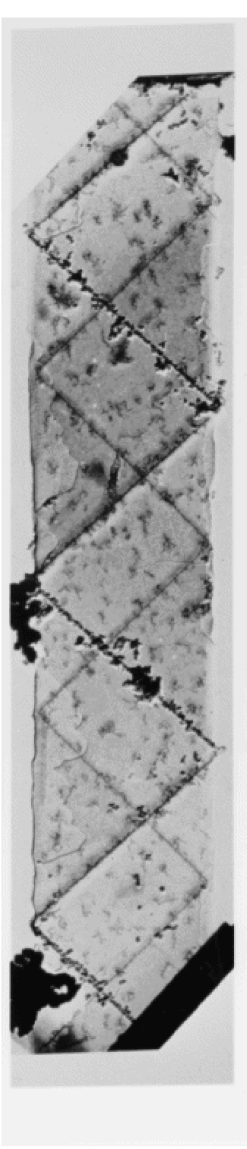
FIG. 1.: Transmission electron micrograph of a tubule with adsorbed Pd/Ni catalyst particles on the surface [4]. The diameter of the tubule is approximately 0.5 $\mu$m. Reprinted from Ref. [19].

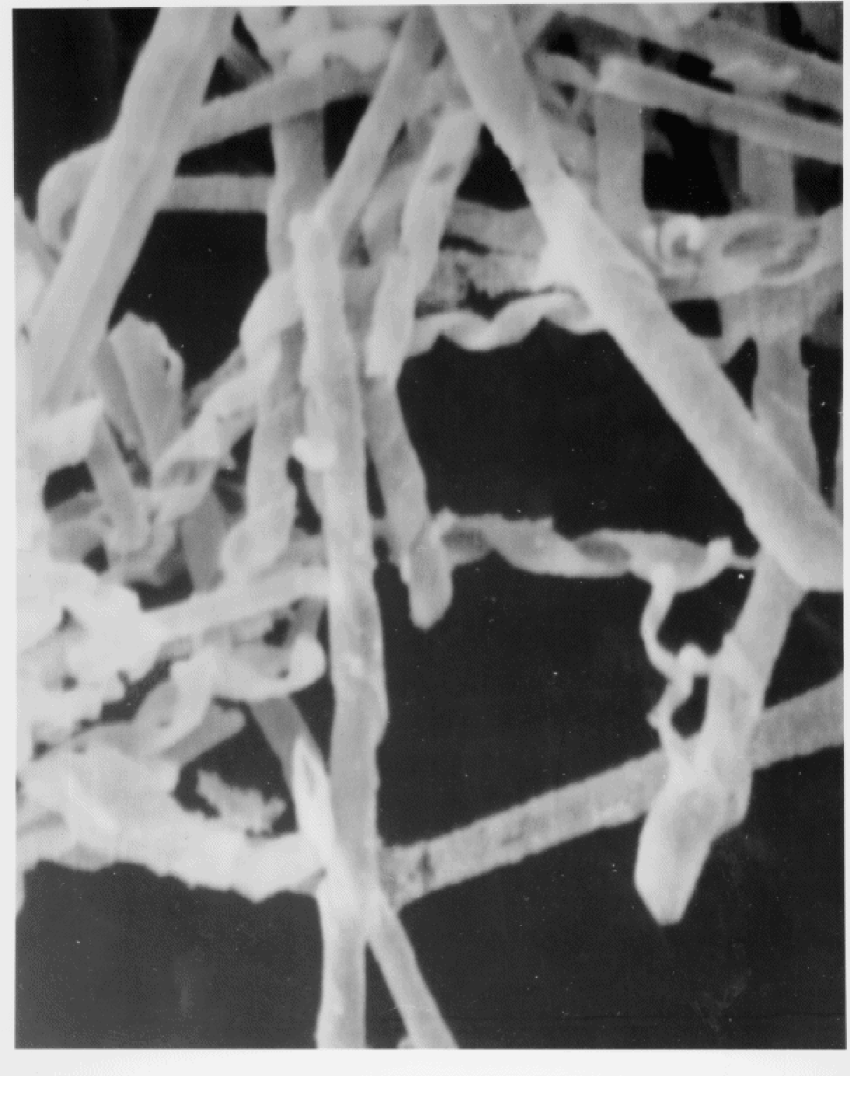
FIG. 2.: Scanning electron micrograph of helical ribbons formed from a racemic mixture of D and L diacetylenic phospholipids. Note that the racemic mixture forms distinct right- and left-handed helical ribbons. The diameter of the helical ribbons is approximately 0.5 $\mu$m. Reprinted from Ref. [9] with permission ©1988 Elsevier Scientific Publishers.

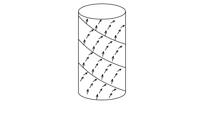
FIG. 3.: Schematic view of the striped pattern in the tilt direction in the modulated state of a tubule. The arrows indicate the direction of the molecular tilt, projected into the local tangent plane.

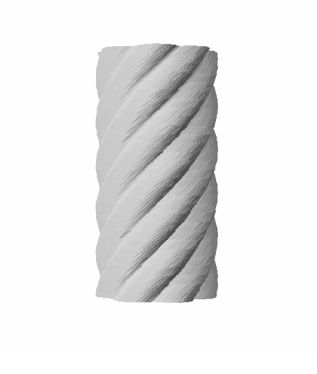
FIG. 4.: Schematic view of the ripples in the curvature in the modulated state of a tubule. The amplitude of the ripples has been exaggerated for clarity.

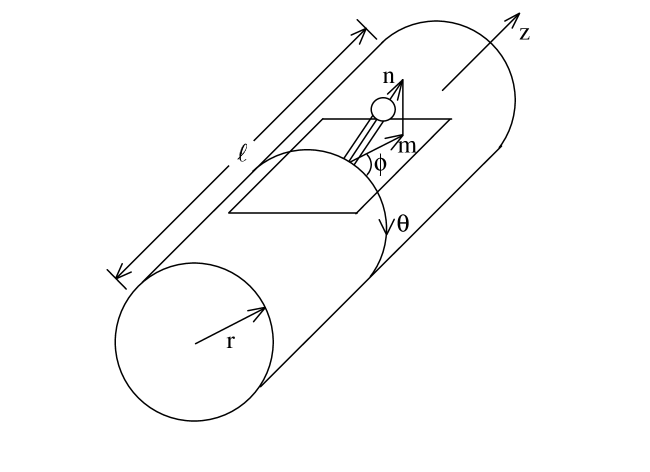
FIG. 5.: Geometry of a tubule with radius $r$ and length $\ell$. Here, $\vec{n}$ is the molecular director, $\vec{m}$ is the projection of $\vec{n}$ into the local tangent plane (normalized to unit magnitude), and $\phi$ is the angle in the tangent plane between $\vec{m}$ and the equator.

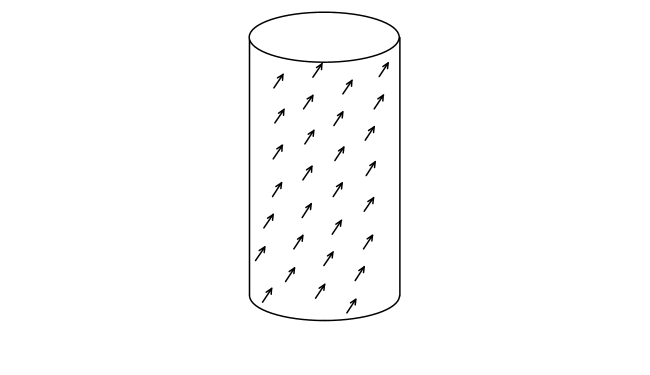
FIG. 6.: Schematic view of a tubule with the uniform tilt direction $\vec{m}=(\cos\phi_{0},\sin\phi_{0})$, as indicated by the arrows.

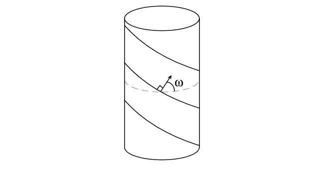
FIG. 7.: Definition of the angle $\omega$, which gives the direction of the stripes and the domain walls on a tubule with respect to the equator.

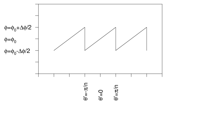
FIG. 8.: Ansatz for the tilt direction $\phi(\theta,z)$, in terms of the coordinate $\theta^{\prime}\equiv\theta+(z/r)\tan\omega$.

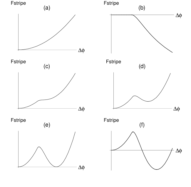
FIG. 9.: Graphical minimization of the stripe free energy $F_{\rm stripe}$ as a function of $\Delta\phi$, as discussed in the text. $F_{\rm stripe}$ is the sum of the two terms plotted in (a) and (b). (c) For large $\nu$, the only minimum is the uniform state with $\Delta\phi=0$. (d) As $\nu$ decreases, another minimum develops for $\Delta\phi\neq 0$. (e) At $\nu=\nu_{c}$, there is a first-order transition from the uniform state ($\Delta\phi=0$) to the modulated state ($\Delta\phi=\Delta\phi_{c}$). (f) For $\nu<\nu_{c}$, the modulated state becomes the absolute minimum of the free energy.

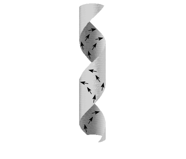
FIG. 10.: Schematic view of a helical ribbon, with a variation in the tilt direction across the width of the ribbon. The arrows represent the tilt direction on one side of the bilayer.

FIG. 11.: Plots of the ripple shapes, as a function of the coordinate $s^{\prime}$ normal to the ripples. For small $\Delta\phi$, the dominant contribution is symmetric under $s^{\prime}\rightarrow-s^{\prime}$, but corrections are asymmetric. (a) $h_{1}<0$ and $h_{2}=0$. (b) $h_{2}\Delta\phi=0.3h_{1}.$ (c) $h_{2}\Delta\phi=h_{1}.$

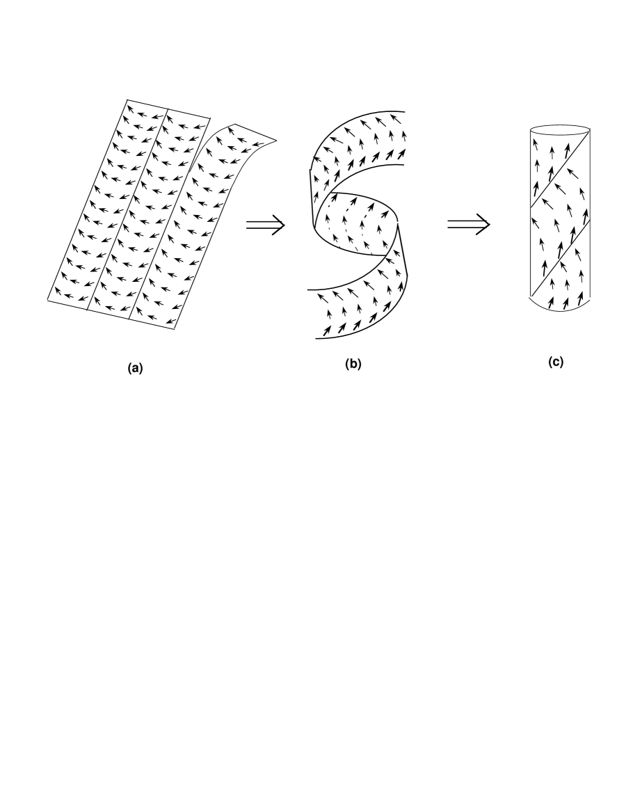
FIG. 12.: Scenario for the kinetic evolution of flat membranes into tubules, as discussed in the text. (a) When a membrane is cooled into a tilted phase, it develops stripes in the tilt direction, and then breaks up along the domain walls to form ribbons. (b) Each ribbon twists in solution to form a helix. (c) A helical ribbon may remain stable, or may grow wider to form a tubule. Reprinted from Ref. [37] with permission ©1994 American Association for the Advancement of Science.

- [1] P. Yager and P. Schoen, Mol. Cryst. Liq. Cryst. 106, 371 (1984).
- [2] J. M. Schnur, Science 262, 1669 (1993).
- [3] R. Shashidhar and J. M. Schnur, in Self-Assembling Structures and Materials (American Chemical Society Books, Washington, 1994), p. 455.
- [4] T. Gulik-Krzywicki and J. M. Schnur (unpublished).
- [5] M. Markowitz and A. Singh, Langmuir 7, 16 (1991).
- [6] D. S. Chung, G. B. Benedek, F. M. Konikoff, and J. M. Donovan, Proc. Natl. Acad. Sci. USA 90, 11341 (1993).
- [7] T. Tachibana, S. Kitazawa, and H. Takeno, Bull. Chem. Soc. Jpn. 43, 2418 (1970).
- [8] N. Nakashima, S. Asakuma, and T. Kunitake, J. Am. Chem. Soc. 107, 509 (1985).
- [9] A. Singh et al., Chem. Phys. Lipids 47, 135 (1988).
- [10] P.-G. de Gennes, C. R. Acad. Sci. Paris 304, 259 (1987).
- [11] J. S. Chappell and P. Yager, Biophys. J. 60, 952 (1991).
- [12] M. A. Markowitz, J. M. Schnur, and A. Singh, Chem. Phys. Lipids 62, 193 (1992).
- [13] T. C. Lubensky and J. Prost, J. Phys. II (France) 2, 371 (1992).
- [14] J. H. Georger et al., J. Am. Chem. Soc. 109, 6169 (1987).
- [15] W. Helfrich and J. Prost, Phys. Rev. A 38, 3065 (1988).
- [16] Ou-Yang Zhong-can and Liu Ji-xing, Phys. Rev. Lett. 65, 1679 (1990); Phys. Rev. A 43, 6826 (1991).
- [17] J. S. Chappell and P. Yager, Chem. Phys. Lipids 58, 253 (1991); P. Yager, J. Chappell, and D. D. Archibald, in Biomembrane Structure and Function—The State of the Art, edited by B. P. Gaber and K. R. K. Easwaran (Adenine Press, Schenectady, NY, 1992).
- [18] P. Nelson and T. Powers, Phys. Rev. Lett. 69, 3409 (1992); J. Phys. II (France) 3, 1535 (1993).
- [19] J. V. Selinger and J. M. Schnur, Phys. Rev. Lett. 71, 4091 (1993).
- [20] S. A. Langer and J. P. Sethna, Phys. Rev. A 34, 5035 (1986).
- [21] G. A. Hinshaw, R. G. Petschek, and R. A. Pelcovits, Phys. Rev. Lett. 60, 1864 (1988); G. A. Hinshaw and R. G. Petschek, Phys. Rev. A 39, 5914 (1989).
- [22] A. E. Jacobs, G. Goldner, and D. Mukamel, Phys. Rev. A 45, 5783 (1992).
- [23] T. C. Lubensky and F. C. MacKintosh, Phys. Rev. Lett. 71, 1565 (1993).
- [24] C.-M. Chen, T. C. Lubensky, and F. C. MacKintosh, Phys. Rev. E 51, 504 (1995).
- [25] A. Tardieu, V. Luzzati, and F. C. Reman, J. Mol. Biol. 75, 711 (1973).
- [26] J. A. N. Zasadzinski, J. Schneir, J. Gurley, V. Elings, and P. K. Hansma, Science 239, 1013 (1988).
- [27] D. R. Nelson and L. Peliti, J. Phys. (Paris) 48, 1085 (1987); see also H. S. Seung and D. R. Nelson, Phys. Rev. A 38, 1005 (1988).
- [28] R. Treanor and M. D. Pace, Biochim. Biophys. Acta 1046, 1 (1990).
- [29] S. L. Brandow, D. C. Turner, B. R. Ratna, and B. P. Gaber, Biophys. J. 64, 898 (1993).
- [30] See also E. Sackmann, H.-P. Duwe, and W. Pfeiffer, Physica Scripta T25, 107 (1989).
- [31] B. N. Thomas, C. R. Safinya, R. J. Plano, and N. A. Clark, Science 267, 1635 (1995).
- [32] W. Helfrich, Z. Naturforsch. 28c, 693 (1973).
- [33] C.-M. Chen and F. C. MacKintosh, Europhys. Lett. 30, 215 (1995).
- [34] P. Yager, P. E. Schoen, C. Davies, R. Price, and A. Singh, Biophys. J. 48, 899 (1985).
- [35] B. N. Thomas, personal communication.
- [36] F. C. MacKintosh and T. C. Lubensky, Phys. Rev. Lett. 67, 1169 (1991).
- [37] J. M. Schnur et al., Science 264, 945 (1994).
- [38] X. Qiu, J. Ruiz-Garcia, K. J. Stine, C. M. Knobler, and J. V. Selinger, Phys. Rev. Lett. 67, 703 (1991).
- [39] G. Nounesis et al., preprint.
- [40] A. S. Rudolph and T. G. Burke, Biochim. Biophys. Acta 902, 349 (1987).
- [41] B. M. Peek, J. H. Callahan, K. Namboodiri, A. Singh, and B. P. Gaber, Macromolecules 27, 292 (1994).