Orbital contribution to the magnetic properties of iron as a function of dimensionality

Abstract

The orbital contribution to the magnetic properties of Fe in systems of decreasing dimensionality (bulk, surfaces, wire and free clusters) is investigated using a tight-binding hamiltonian in an $s,p,$ and $d$ atomic orbital basis set including spin-orbit coupling and intra-atomic electronic interactions in the full Hartree-Fock (HF) scheme, i.e., involving all the matrix elements of the Coulomb interaction with their exact orbital dependence. Spin and orbital magnetic moments and the magnetocrystalline anisotropy energy (MAE) are calculated for several orientations of the magnetization. The results are systematically compared with those of simplified hamiltonians which give results close to those obtained from the local spin density approximation. The full HF decoupling leads to much larger orbital moments and MAE which can reach values as large as 1$\mu_{B}$ and several tens of meV, respectively, in the monatomic wire at the equilibrium distance. The reliability of the results obtained by adding the so-called Orbital Polarization Ansatz (OPA) to the simplified hamiltonians is also discussed. It is found that when the spin magnetization is saturated the OPA results for the orbital moment are in qualitative agreement with those of the full HF model. However there are large discrepancies for the MAE, especially in clusters. Thus the full HF scheme must be used to investigate the orbital magnetism and MAE of low dimensional systems.

I Introduction

The magnetic properties of reduced dimensionality systems is an area of growing interest both for experimentalists and theoreticians. Indeed, the spin magnetic moment of an atom is strongly dependent on its environment, in particular, on its coordination number. It usually increases when the latter decreases and may even appear in small clusters for some transition metals which are not magnetic in the bulk phase Cox94 ; Guirado98a ; Guirado98b ; Barreteau00a . Another quantity playing a key role in technological applications, like magnetic recording, is the magnetocrystalline anisotropy energy (MAE) which is responsible for the tendency of the magnetization to align along particular directions. It is well known that this MAE is very small in the bulk phase of ferromagnetic transition metals but may increase by several orders of magnitude when the dimensionality or the symmetry of the system is reduced. The most striking specific property of low dimensional systems is perhaps the appearance of a sizable orbital contribution to the magnetic moment which, on the contrary, is practically quenched in bulk systems. Obviously, the influence of intra-atomic Coulomb interactions and spin-orbit coupling, responsible for Hund’s rules in the free atom, become more and more important when the band width due to electron delocalization decreases and both the spin and orbital moments should tend to their atomic values. Furthermore, the interest for the orbital moment has been stimulated by a newly acquired physical technique, the X-ray Magnetic Circular Dichroism (XMCD), which is able to resolve spin and orbital moments. Such experiments have been carried out by Gambardella et al. Gambardella02 ; Gambardella03 who have indeed measured orbital moments as large as 0.68$\mu_{B}$ for Co chains on Pt(997) and 1.1$\mu_{B}$ for a Co adatom on Pt(111), the corresponding MAE being 2meV and 9meV per Co atom, respectively. Moreover XMCD experiments carried out on iron clustersEdmonds00 ; Binns01 have shown that the orbital moment is much more enhanced than the spin moment as the size is reduced.

From the theoretical point of view, the spin moment can be obtained in the Local Spin Density Approximation (LSDA) or with a Stoner-like Tight-Binding (TB) hamiltonian Autes06 but the spin orientation is arbitrary. This is not true when spin-orbit coupling is taken into account and, consequently, the MAE and the orbital moment no longer vanish. However, in these schemes the hamiltonian depends only on the total spin density (LSDA) or spin population at each site (TB) and not on their repartition between the orbital states. In other words electronic interactions are averaged which yields underestimated values of MAE and orbital moments, eventhough these quantities increase when the dimensionality is reducedXie04 . Eriksson et al. Eriksson90 have proposed to correct this drawback by adding to the total energy a term proportional to $-\frac{1}{2}\langle{\bf L}\rangle^{2}$ which will be referred to as the Orbital Polarization Ansatz (OPA) in the following. This obviously tends to increase $\langle{\bf L}\rangle$ but is not really justified.

A more rigorous way of obtaining the correct distribution of electrons between the $d$ orbital states of opposite magnetic quantum numbers $m$ is to take into account all intra-atomic terms in the Hartree-Fock (HF) decoupling of the two-body operators representing electron-electron interactions in the hamiltonian with the exact expression of the matrix elements $U_{\gamma_{1}\gamma_{2}\gamma_{3}\gamma_{4}}$ of $e^{2}/|{\bf r}-{\bf r^{\prime}}|$ as a function of the three Racah parameters A, B and C relative to $d$ atomic orbitals $\gamma_{\alpha}$. Note that, when using L(S)DA or a TB hamiltonian parametrized by fits on L(S)DA calculations, some electronic interactions are implicitly already included. This is usually accounted for by assuming that on each atom all spin-orbitals (all spin-orbitals with the same spin) are equally populated in LDA (LSDA).

Some attempts have been made in this direction. However, most often the terms involving three and four different orbitals have been neglected which destroys the rotational invariance of the interaction hamiltonian Nicolas06 unless appropriate averages of the matrix elements with two different orbitals are done Anisimov93 ; Wierzbowska05 . Nevertheless there exists in the literature some scarce calculations in which all matrix elements of the Coulomb interactions were taken into accountLiechtenstein95 ; Shick04 but, at least to our knowledge, no systematic study comparing this complete HF scheme to the OPA has been carried out save for our preliminary work on the Fe monatomic wireDesjonqueres07 in the TB approximation with an atomic orbital basis set restricted to $d$ orbitals. Such a comparison is indeed very interesting since Solovyev et al. Solovyev98 have shown, in an elegant work, that the OPA cannot be derived analytically from the full HF hamiltonian except in some very special cases. In the present work we generalize our previous studyDesjonqueres07 , on the one hand, by using a realistic description of the electronic states including $sp-d$ hybridization in order to get quantitative results and, on the other hand, by investigating systems with various dimensionalities (bulk, surfaces, wire, clusters).

The paper is organized as follows. The formalism and the choice of parameters for Fe are described in Sec.II. Secs.III and IV are devoted to bulk and surfaces of bcc iron, respectively. Our results concerning the monatomic wire and some clusters are given in Secs.V and VI. Finally conclusions are drawn in Sec.VII.

II Formalism

The hamiltonian of the system is written as:

$$H=H_{TB}+H_{so}+\Delta H_{int}$$ (1)

$H_{TB}$ is a tight-binding hamiltonian parametrized for the non magnetic state by fitting ab-initio calculations in the LDA (Local Density) or GGA (Generalized Gradient) approximation, $H_{so}$ is the spin-orbit coupling term and $\Delta H_{int}$ describes the change in electronic interactions with respect to $H_{TB}$.

We choose a non orthogonal basis set made of the real s, p and d valence atomic orbitals (i.e. cubic harmonics for reasons which will become clear in the following) centered at each site i. They are denoted by $\lambda$ and $\mu$ indices ($\lambda,\mu=1,9$) and numbered as follows: $s,p_{x},p_{y},p_{z},d_{xy},d_{yz},d_{zx},d_{x^{2}-y^{2}},d_{3z^{2}-r^{2}}$ (the x, y, z coordinates being taken along the crystal axes) with overlap integrals $S^{\lambda\mu}_{ij}$ depending on the bonding direction ${\bf R}_{ij}$. The hamiltonian $H_{TB}$ is completely determined by its intra-atomic matrix elements (i.e., the s, p and d atomic levels) $\epsilon_{i\lambda}$ and its inter-atomic matrix elements (i.e., the hopping integrals) $\beta^{\lambda\mu}_{ij}({\bf R}_{ij})$. The functions $S^{\lambda\mu}_{ij}({\bf R}_{ij})$ and $\beta^{\lambda\mu}_{ij}({\bf R}_{ij})$ are given by the same analytical expressions as a function of two sets (one for overlap and one for hopping) of ten Slater-Koster (SK) integrals ($ss\sigma,sp\sigma,sd\sigma,pp\sigma,pp\pi,pd\sigma,pd\pi,dd\sigma,dd\pi,dd\delta$) and of the direction cosines of ${\bf R}_{ij}$ Slater54 . Following the (MP) scheme developed by Mehl and Papaconstantopoulos Mehl96 , the atomic levels depend on the atomic environment (number of neighbors and interatomic distances) while the SK integrals are functions of $R_{ij}$ only. The atomic levels and the SK integrals are written as analytic functions depending on a number of parameters which are determined by a least mean square fit of the results of ab-initio LDA or GGA electronic structure (band structure and total energy) calculations. These parametrizations will be denoted respectively as TBLDA and TBGGA in the following: the analytical forms of the functions can be found in Ref.Mehl96, and the numerical values of the parameters for Fe in Ref.Papaweb, .

The spin-orbit coupling hamiltonian $H_{so}$ is given by:

$$H_{so}=\xi{\bf L}.{\bf S}$$ (2)

where ${\bf L}$ and ${\bf S}$ are the orbital and spin momentum operators, respectively. Due to the local character of this interaction, only the intra-atomic matrix elements between d spin-orbitals have been taken into account. For more details the reader is referred to Ref.Autes06, where $\xi$ has been determined ($\xi=0.06$eV).

Only the intra-atomic electronic interactions are taken into account. For d electrons they are written in the Hartree-Fock approximation, i.e.:

$$H_{\text{int},dd}^{\text{HF1}}= \displaystyle\sum_{\begin{subarray}{c}i\gamma_{1}\gamma_{2}\gamma_{3}\gamma_{4}\\ \sigma\sigma^{\prime}\end{subarray}}\Big{(}U_{\gamma_{4}\gamma_{2}\gamma_{3}\gamma_{1}}\langle n_{i\gamma_{3}\gamma_{4}}^{\sigma\sigma}\rangle c_{i\gamma_{2}\sigma^{\prime}}^{{\dagger}}c_{i\gamma_{1}\sigma^{\prime}}$$ (3)

$$-U_{\gamma_{4}\gamma_{2}\gamma_{1}\gamma_{3}}\langle n_{i\gamma_{3}\gamma_{4}}^{\sigma^{\prime}\sigma}\rangle c_{i\gamma_{2}\sigma^{\prime}}^{{\dagger}}c_{i\gamma_{1}\sigma}\Big{)}$$

as a function of the net density matrix $\langle n_{i\gamma_{1}\gamma_{2}}^{\sigma\sigma^{\prime}}\rangle=\langle c_{i\gamma_{2}\sigma^{\prime}}^{{\dagger}}c_{i\gamma_{1}\sigma}\rangle$ when all intra-atomic matrix elements of the Coulomb interactions, i.e.:

$$U_{\gamma_{1}\gamma_{2}\gamma_{3}\gamma_{4}}=\langle\gamma_{1}(\bm{r}),\gamma_{2}(\bm{r^{\prime}})|\frac{e^{2}}{|\bm{r-r^{\prime}}|}|\gamma_{3}(\bm{r}),\gamma_{4}(\bm{r^{\prime}})\rangle$$ (4)

where $\gamma_{i}$ are a set of atomic d orbitals, are retained (HF1 model of Ref.Desjonqueres07, ). These matrix elements can be expressed as a function of the three Racah parameters A, B, C Griffith61 . This hamiltonian is rotationally invariant in spatial as well as in spin coordinates since the spin-flip terms (i.e., with $\sigma^{\prime}\neq\sigma$ ) arising from spin-orbit coupling are present in $H_{\text{int},dd}^{\text{HF1}}$.

Let us now comment on our choice for the basis set. Obviously, when all terms are present in $H_{\text{int},dd}^{\text{HF1}}$, the results do not depend on the basis set. This may not be the case when some matrix elements are omitted. For instance, in a common approximation, the terms involving three and four different orbitals are neglected Anisimov93 ; Czyzyk94 . When using a basis set made of spherical harmonics denoted by the value of the quantum number m, the three and four orbital terms are a function of both B and C. Therefore if these terms are neglected without changing the one and two different orbital matrix elements, the rotational invariance is destroyed unless we set B=C=0, in which case the Coulomb type integrals $U_{mm^{\prime}mm^{\prime}}=A$ are completely isotropic and the exchange integrals $U_{mm^{\prime}m^{\prime}m}$ vanish. This model is thus oversimplified if we want to study spin and orbital magnetism. On the contrary when the basis set is built from cubic harmonics, the three and four orbital matrix elements are a function of B only Griffith61 . When these terms are neglected the rotational invariance is conserved only if B is set equal to zero. Then in this model $U_{\lambda\mu\lambda\mu}=A+C$ and $U_{\lambda\mu\mu\lambda}=C$ for any pair $\lambda,\mu$ of different d orbitals. This model can describe correctly spin magnetism by an appropriate choice of the parameters but cannot really account for orbital magnetism as shown in Ref.Desjonqueres07, on a simple model. This suggests to redefine the parameters determining the HF1 hamiltonian as U, J, B with $U=(1/4)\sum_{\mu,\mu\neq\lambda}U_{\lambda\mu\lambda\mu}$ and $J=(1/4)\sum_{\mu,\mu\neq\lambda}U_{\lambda\mu\mu\lambda}$, the sums being independent of $\lambda$. These average values of Coulomb and exchange interactions are given by $U=A-B+C$ and $J=5B/2+C$. Thus we expect that in the HF1 model the orbital magnetism, which is sensitive to the anisotropy of electronic interactions, is mainly governed by B similarly to what is assumed in the orbital polarization ansatz.

In the following we will consider also the HF2 model of Ref.Desjonqueres07, which is obtained from HF1 by setting B=0 and sometimes called the U,J model. Finally a Stoner-like model called HF3 can be derived from HF1 under the following assumptions: i) the net density matrix $\langle n_{i\lambda\mu}^{\sigma\sigma^{\prime}}\rangle$ is diagonal with elements equal to the net occupation numbers $n_{i\lambda\sigma}$, ii) on each site i the exact $n_{i\lambda\sigma}$ are replaced by their average value $n_{i\sigma}=1/5\sum_{\lambda}n_{i\lambda\sigma}$. Then it is easily shown (see Appendix A) that the simplified hamiltonian can be written:

$$H_{\text{int},dd}^{\text{HF3}}=\sum_{i\lambda\sigma}(U_{\text{eff}}N_{i,d}-\sigma I_{dd}M_{i,d}/2)c_{i\lambda\sigma}^{{\dagger}}c_{i\lambda\sigma}.$$ (5)

where $U_{\text{eff}}=(9U-2J)/10$, $I_{dd}=(U+6J)/5$ is the $d$ Stoner parameter, $N_{i,d}(M_{i,d})$ are the net d total population (spin momentum) at site i and $\sigma=+1(-1)$ for majority (minority) spin. Note that the above conditions are approximately obeyed for bulk transition metals but become questionable when the symmetry is lowered.

We must not forget that some electronic interactions are already included in $H_{TB}$ since this hamiltonian has been parametrized by fitting LDA and GGA calculations. This is taken into account following the treatment done in the ”around mean field” LDA+U theory Czyzyk94 , i.e.,

$$\Delta H_{\text{int},dd}=H_{\text{int},dd}(n_{i\lambda\mu}^{\sigma\sigma^{\prime}})-H_{\text{int},dd}({\bar{n}}_{i}\delta_{\lambda\mu}\delta_{\sigma\sigma^{\prime}})$$ (6)

with ${\bar{n}}_{i}=\sum_{\lambda\sigma}n_{i\lambda\sigma}/10$, whatever the model (HF1, HF2 or HF3).

Finally, the small exchange splittings of the s and p levels due to the spin polarization of d electrons is treated with a Stoner-like model and a Stoner parameter $I_{sd}=I_{pd}=I_{dd}/10$, i.e.:

$$\Delta H_{\text{int},s(p)d}=-\sigma I_{s(p)d}M_{i,d}/2$$ (7)

so that:

$$\Delta H_{\text{int}}=\Delta H_{\text{int},sd}+\Delta H_{\text{int},pd}+\Delta H_{\text{int},dd}$$ (8)

From the above discussion it is clear that HF2 differs from HF1 by terms proportional to $B$, this is also true for HF3 as far as this hamiltonian is justified. Eriksson et al.Eriksson90 have proposed to introduce an OPA term to account for this difference. This term is written in meanfield $\Delta E_{\text{OP}}=-\frac{1}{2}B\sum_{i}\langle\bm{L}_{i}\rangle^{2}$ which reduces to $-\frac{1}{2}B\sum_{i}\langle L_{iZ}\rangle^{2}$ when the spin and orbital moment $\langle\bm{L}_{i}\rangle$ are collinear with the axis $Z$ which is verified along high symmetry directions (in the following X, Y, Z will denote the framework in which Z is the magnetization direction). The corresponding hamiltonian is then:

$$H_{\text{OP}}=-B\sum_{i\lambda\mu\sigma}\langle L_{iZ}\rangle[L_{iZ}]_{\lambda\mu}c_{i\lambda\sigma}^{{\dagger}}c_{i\mu\sigma}$$ (9)

where $[L_{iZ}]_{\lambda\mu}$ are the matrix elements of the local orbital moment operator $L_{iZ}$. Note that in the basis of cubic harmonics $[L_{iZ}]_{\lambda\mu}$ is not diagonal Autes06 . In the following we also compare the results obtained with HF1 to those derived from HF2 or HF3 to which the OPA term has been added.

As in our previous work Autes06 we use the HF3 model to determine the Stoner parameter $I_{dd}$ so as to reproduce as closely as possible the variation of the bulk spin magnetic moment as a function of the interatomic distance that can be obtained from a spin polarized DFT calculation. This gives $I_{dd}=1.eV$. Finally from Fig.1 of the recent work by Solovyev Solovyev05 it can be deduced that $U\simeq J$. As a consequence we have taken $U=J=5I_{dd}/7=0.71eV$ and similarly to most previous works $B=0.14J$ Solovyev05 .

III Spin and orbital magnetism in bulk bcc iron

Let us first consider the bulk bcc phase of Fe and compare the results obtained with HF1 and HF3 using the TBGGA parameters. Indeed we do not expect strong differences between HF2 and HF3 for the following reasons. First, in the absence of the small perturbation due to spin-orbit coupling, the intra-atomic density matrix is diagonal for symmetry reasons in cubic crystals. Second, the populations of the different orbitals with a given spin are rather similar in the bulk.

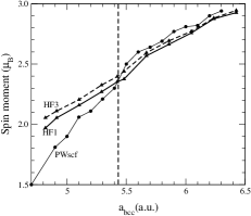
Figure 1: Spin magnetic moment of bulk bcc iron as a function of the cubic lattice parameter from PWscf ab initio calculations, HF1 and HF3 models. The dashed straight line corresponds to the experimental equilibrium lattice parameter.

Calculations show that the equilibrium lattice parameter (5.35a.u.) is close to the experimental value (5.43a.u.) and that the variation of the spin moment with the lattice parameter is almost the same with the HF1 and HF3 models. For instance the spin moments are 2.34$\mu_{B}$ and 2.39$\mu_{B}$ with HF1 and HF3, respectively (see Fig.1) at the experimental equilibrium lattice parameter. On the opposite the orbital moment is significantly enhanced with the HF1 model (see Fig.2) and in very good agreement with experiment (0.09$\mu_{B}$) Landolt86 .

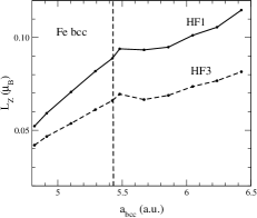
Figure 2: Orbital magnetic moment of bulk bcc iron as a function of the cubic lattice parameter from the HF1 and HF3 models. The dashed straight line corresponds to the experimental equilibrium lattice parameter.

IV Spin and orbital magnetism at bcc iron Surfaces

We have applied the HF1 and HF3 models to the study of the $(001)$ and $(110)$ surfaces of bcc iron. The surfaces are modelled by slabs of 15 atomic layers which is sufficient to avoid interactions between the two surfaces and to recover the bulk behaviour on the central layer. Interlayer relaxations are neglected in all calculations and the interatomic distance is set equal to the experimental one ($d_{\text{bulk}}^{\text{exp}}=4.69$a.u.). In such systems some atoms have a reduced coordination compared to the bulk and therefore charge transfers are expected. In order to avoid unphysically large charge transfers at the surface we have used a penalty function (see Appendix B) which consists in adding to the energy functional a term of the type:

$$E^{\text{pen}}_{\text{LCN}}=\lambda^{\text{pen}}_{\text{LCN}}\sum_{i}(\Delta q_{i})^{2}$$ (10)

$\Delta q_{i}=q_{i}-q_{0}$ where $q_{i}$ is the Mulliken charge of site $i$, $q_{0}$ the valence charge and $\lambda^{\text{pen}}_{\text{LCN}}$ the penalization factor which must be taken large enough to ensure local charge neutrality (in practice one takes $\lambda^{\text{pen}}_{\text{LCN}}=2.5$eV which gives charge transfers below 0.1 electron per atom.). The local charges $q_{i}$ are expressed as a function of the tight-binding expansion coefficients $C_{i\lambda\sigma}^{n}$ of the eigenfunctions $n$ with respect to the atomic orbitals

$$q_{i}=\text{Re}\Bigg{(}\sum_{\begin{subarray}{c}\lambda j\mu\sigma\\ n\end{subarray}}f_{n}C_{i\lambda\sigma}^{n\star}C_{j\mu\sigma}^{n}S_{ij}^{\lambda\mu}\Bigg{)}$$ (11)

where $f_{n}$ is the occupation factor and depends on the type of system. In periodic systems such as surfaces, a broadening technique is used and $f_{n}=f(\varepsilon_{n})$ is equal to the Fermi function at the energy level $\varepsilon_{n}$ for a given temperature.

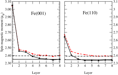
Figure 3: Variation of the spin magnetic moment (per atom) on successive layers of $(001)$ and $(110)$ slabs (with 15 atomic layers) of bcc Fe obtained from HF1 (full lines) and HF3 (dashed lines) models. Layer 1 corresponds to the outermost layer and layer 8 to the central layer. The horizontal lines correspond to the bulk limit.

A standard iterative scheme is set up until input and output intra-atomic density matrix elements differ by less than $10^{-4}$ electron per atom and the total energy of the slab does not change by more than $10^{-4}$eV. We have calculated the spin and orbital moments decomposed on each atomic layer of the $(001)$ and $(110)$ slabs. The results of our calculations are shown in Fig.3 and Fig.4. As expected the spin magnetic moment is enhanced in the vicinity of the surface, this reinforcement being more pronounced for the $(001)$ for which the outermost layer is almost saturated, than for the $(110)$ slab since the $(001)$ surface is more open than the $(110)$. The convergence to the bulk spin moment is also slightly faster for the $(110)$ slab than for the $(001)$ slab. Finally, apart from a small shift of the bulk spin moment between HF1 (2.34$\mu_{B}$) and HF3 (2.39$\mu_{B}$) the two models lead to very similar results. Let us also note that we have verified that the spin moment is almost independent on the magnetization orientation.

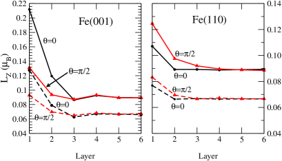
Figure 4: Variation of the component of the local orbital magnetic moment on the magnetization direction as a function of the atomic layer in the $(001)$ and $(110)$ slabs (15 layers) for a magnetization perpendicular ($\theta=0$) and parallel ($\theta=\pi/2$) to the surface from HF1 (full lines) and HF3 (dashed lines) models. For in-plane magnetization the dependence of the orbital moment on the orientation in the plane is negligible.

At surfaces the orbital moment is also strongly enhanced. However in contrast to the spin moment the type of model used is now crucial. Indeed the enhancement of the orbital magnetization at the surface is much more pronounced with the HF1 model than with HF3. For magnetization perpendicular to the surface one finds values of $\langle L_{iZ}\rangle$ as large as 0.21$\mu_{B}$ on the outermost layer of the $(001)$ surface with the HF1 model, while it is 0.127$\mu_{B}$ with the HF3 model. The orbital moment is therefore 2.40 larger at the surface than it is in the bulk (0.088$\mu_{B}$) with HF1 while it is slightly less than twice larger with HF3. The orbital polarization effect is therefore amplified at the surface: a 63% increase of the surface orbital moment between HF3 and HF1 is obtained which must be compared to 33% in the bulk (0.088$\mu_{B}$ with HF1 and 0.066$\mu_{B}$ with HF3). This general trend is also observed on the $(110)$ surface though not so pronounced. Finally, contrary to the case of the spin moment the orbital moment $\langle L_{iZ}\rangle$ depends sensitively on the magnetization direction and moreover the two surfaces behave differently. It is found that the orbital moment is noticeably larger for magnetization perpendicular to the surface in the case of the $(100)$ slabs, while a slight increase of the orbital moment is observed for in-plane magnetization in the case of $(110)$ slabs. In that respect HF1 and HF3 models lead to very similar behaviors. Finally one should point out that for in-plane magnetization the dependence of the orbital moment on the orientation in the plane is negligible.

V Magnetic properties of an iron monatomic wire

In a preliminary work Desjonqueres07 we already investigated the orbital contribution to the magnetic properties of the Fe monatomic wire and checked the ability of the OPA to account for the existence of large orbital moments in one-dimensional structures by comparing to the results obtained from a full Hartree-Fock decoupling of intra-atomic electronic interactions. To this aim we used a simple tight-binding model in which only d electrons were taken into account. However in this model only the self-consistent solution(s) of the hamiltonian could be determined but not the total energy. Furthermore the number of d electrons was fixed. On the contrary, the use of a s, p, d basis set allows a charge redistribution between sp and d orbitals as a function of the interatomic distance $d$ and the determination of the total energy. In the following we present the results obtained for a monatomic Fe wire with this realistic basis set using the TBLDA MP parameters for reasons which have been discussed in Ref.Autes06, . This will enable us to confirm the qualitative trends obtained in the previous model and to get quantitative results.

We have computed the total energy, the spin and orbital magnetic moments, the band structure and the electronic transmission factor as a function of the interatomic distance for the different models, i.e., HF1 and HF2 or HF3 without and with OPA. The results show that the equilibrium distance is quite insensitive to the model chosen and is close to 4.05a.u. (2.14Å) with a slight dispersion smaller than 0.02a.u.. The spin magnetic moment is quite independent on the direction of magnetization. This moment is also almost unchanged when the OPA term is added to HF2 or HF3. Finally, while the spin moment saturates between 3.7 and 3.8a.u. for HF1 and HF2, this saturation occurs at a shorter distance (between 3.6 and 3.7a.u.) with HF3. Note that these latter results are in much better agreement with ab initio calculations (3.8a.u. Autes06 ) than in the pure d band model.

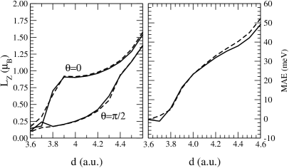
Figure 5: Comparison between the results obtained with the HF2+OPA (full lines) and HF3+OPA (dashed lines) hamiltonians for the monatomic Fe wire as a function of interatomic distance: a) orbital moment for directions of magnetization parallel ($\theta=0$) and perpendicular ($\theta=\pi/2$) to the wire, b) the corresponding magnetocrystalline anisotropy energy.

Let us now compare the orbital magnetic moments and MAE obtained with the various models. The models HF2 and HF3 with (Fig.5) or without OPA give very similar results save for $3.6<d<3.8a.u.$, i.e., the domain of distances for which at least one of these models leads to an unsaturated spin moment. As a consequence we will now limit ourselves to the comparison between the HF1, HF3 and HF3+OPA hamiltonians for magnetizations parallel ($\theta=0$) and perpendicular ($\theta=\pi/2$) to the wire. A glance at Fig.6 confirms, as expected, that HF3 largely underestimates the orbital moment $\langle L_{Z}\rangle$ for both magnetization directions, and the MAE. Adding the OPA to HF3 obviously increases these quantities, however, for the orbital moment the difference with the result derived from HF1 does not keep the same sign as a function of the interatomic distance and is rather large when the spin is not saturated.

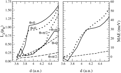
Figure 6: Same caption as Fig.5 but for the HF1 (full lines), HF3 (dashed lines), HF3+OPA (dotted lines) hamiltonians. Note that the curves referring to HF1 correspond to the most stable self-consistent solution for each value of $d$(see text).

It is worthwhile to discuss the results given by HF1 in more details. First at $\theta=0$ a sharp change of slope occurs for $\langle L_{Z}\rangle$ at $d$=3.9a.u.. Let us recall Desjonqueres07 that at $\theta=0$ the wire eigenfunctions corresponding to the almost flat $\delta$ bands located near the Fermi level are a linear combination of d spherical harmonics (with m=2 or m=-2) centered at each site. When d increases from 3.6a.u. the population of the highest energy band m=-2 decreases and vanishes for $d\simeq 3.9a.u.$. This explains the change of slope in the $\langle L_{Z}\rangle$ curve. Note also that for $d>4.3a.u$, two self-consistent solutions are found corresponding to an empty band either with m=2 or m=-2 character and nearly opposite values of $\langle L_{Z}\rangle$. However the solution in which the m=-2 band is empty and $\langle L_{Z}\rangle>0$ is always the most stable one. On the contrary at $\theta=\pi/2$ the character of the eigenfunctions of the $\delta$ bands near the Fermi level is $d_{xy}$ or $d_{x^{2}-y^{2}}$. Up to $d=4.a.u.$ these two bands are quasi degenerate. Then, when $d\geq 4.1a.u.$ two self-consistent solutions are found for which either $d_{xy}$ or $d_{x^{2}-y^{2}}$ are empty but, contrary to what occurs at $\theta=0$, they have almost the same total energy and very similar values of $\langle L_{Z}\rangle$. The change of slope at $d=4.5a.u.$ corresponds to the switch of the ground state from one case (empty $d_{x^{2}-y^{2}}$ band) to the other (empty $d_{xy}$ band).

It is interesting to compare our results with those of our previous works. In Ref.Autes06, we showed, using a Stoner like hamiltonian, that the proportionality relation between the MAE and the anisotropy of the orbital moment proposed by Bruno Bruno89 , by treating the spin-orbit coupling by means of perturbation theory, is almost strictly verified when the interatomic distance in the wire is such that the spin moment is saturated. It is clear from Fig. 6 that this law is not satisfied with HF1 eventhough the MAE has the same sign as $\langle L_{Z}(\theta=0)\rangle-\langle L_{Z}(\theta=\pi/2)\rangle$.

To illustrate the departure from the perturbation theory we have found useful to study the variation of the MAE and orbital magnetization with the angle between the monatomic wire and the magnetization axis. If one starts a calculation from a non symmetric magnetic configuration (different from $\theta=0$ or $\theta=\pi/2$) and let the self-consistent process iterate until convergency it should bring the system towards the easy axis. Therefore one has to find a way to follow the evolution with respect to the angle $\theta$. In order to constraint the angle $\theta$ between the spin moment and the $z$-axis we add a penalty functional

$$E^{\text{pen}}_{\text{ang}}=\lambda^{\text{pen}}_{\text{ang}}(\cos\theta-\cos\theta_{0})^{2}$$ (12)

to the total energy (see Appendix B).

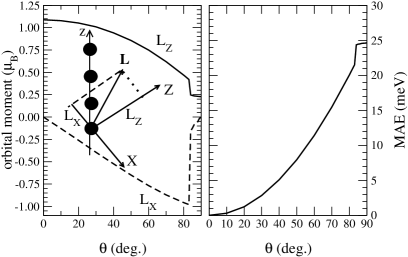
Figure 7: a) Variation of the components of the orbital moment and of the magnetic anisotropy energy as a function of the direction of magnetization given by the angle $\theta$ for a monatomic wire (interatomic distance $d=4.05$a.u.) obtained from HF1.

In practice $\lambda^{\text{pen}}_{\text{ang}}=1$eV ensures that the angle $\theta$ does not deviate by more than $0.1^{\circ}$ from $\theta_{0}$. Fig. 7 shows the results of our calculations with the HF1 model. This clearly shows that the orbital moment and the MAE are strongly modified when the anisotropy of the electronic interactions is taken into account. The MAE and the orbital moment no longer follow a simple $\sin^{2}\theta$ law and moreover present an abrupt variation around $\theta=80^{\circ}$ which corresponds to an electronic transition. Note that the position of this transition strongly depends on the interatomic distance. At larger interatomic distances this transition occurs for smaller $\theta$ angles.

We must emphasize that the qualitative trends put forward in Ref.Desjonqueres07, are also obeyed when the basis set is extended to include s and p orbitals, namely: i) the orbital moment and MAE are largely underestimated with a Stoner-like hamiltonian but they reach numerical values similar to those observed experimentally in one dimensional systems when HF1 is used, ii) adding the OPA to HF2 or HF3 leads to a fair agreement with HF1 for both $\langle L_{Z}\rangle$ and MAE when the spin moment is saturated but this agreement deteriorates in relative value for unsaturated spin polarization.

Finally we show in Fig.8 the band structure obtained with HF1 and HF3 for $\theta=0$ and $\theta=\pi/2$ at the equilibrium distance from which the electronic transmission factor $T(E)$ is deduced by a simple counting of the number of eigenfunctions at a given energyDatabook . Some differences are observed, in particular at $\theta=0$: around the Fermi level the energy domain inside which $T(E)=7$ is narrowed when HF1 is used instead of HF3. Such differences should appear in more complex geometries such as those obtained in the constriction region of break junctions and could have important consequences on magnetoresistance propertiesViret06 .

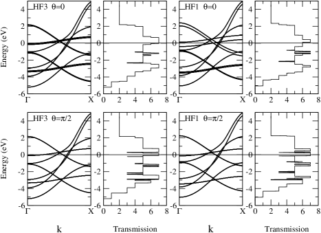
Figure 8: Band structure and the corresponding electronic transmission factor of an iron monatomic wire for magnetizations parallel ($\theta=0$) and perpendicular ($\theta=\pi/2$) to the wire from the HF1 and HF3 models.

VI Magnetic properties of some iron clusters

In the previous sections we have studied 3- (bulk), 2- (surface), and 1- (wire) dimensional periodic systems. To end this work we have investigated zero-dimensional structures, i.e., unsupported clusters. We have considered five clusters with various geometries presented in Fig. 9.

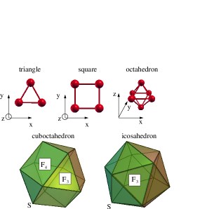
Figure 9: Geometry of the iron clusters. In the case of cuboctahedral and icosahedral geometries each apex $S$ and the centre of the cluster are occupied by an iron atom. $F_{4}$ and $F_{3}$ denote the center of a square and triangular facet, respectively.

Three of these clusters (triangle, square and regular octahedron) are made of geometrically equivalent atoms, while the two others (cuboctahedron and icosahedron) are built from a central atom surrounded by twelve atoms forming the outer shell. Since it was shown in the previous section that HF2 and HF3 basically give the same results for saturated systems we have restricted our study to the three models: HF1, HF3 and HF3+OPA. In a first step we have minimized the total energy with respect to the nearest neighbour distance. We only consider an homogenous contraction of the cluster and ignore Jahn Teller distorsions. Note that the discrete levels of the clusters have been filled with electrons up to the highest occupied level (HOMO), i.e., the occupation factor $f_{n}=1$ or $0$ except when the HOMO level is degenerate and not completely filled. In the latter case the different wave functions corresponding to the HOMO level have been equally populated in order to preserve the cluster symmetry. Similarly to the case of surfaces a penalization function has been used to avoid large charge transfers (see Appendix B).

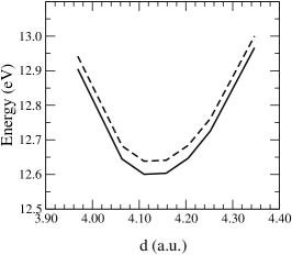
Figure 10: Total energy as a function of the interatomic distance of a triangular iron cluster from HF1 (full line) and HF3 (dashed line) models. Note that the HF3+OPA curve would be undistinguishable from the HF3 one.

As illustrated in Fig. 10 the equilibrium interatomic distance is almost insensitive to the type of hamiltonian. We also checked that the magnetization orientation does not influence the equilibrium distance either. As a consequence the relaxed structures have been determined from HF3 calculations and a magnetization along a high symmetry direction (see Fig. 9). The results are summarized in Table 1. For all clusters a contraction of the equilibrium bond-length with respect to the calculated bulk one ($d_{\text{bulk}}=4.63$a.u.) is obtained and the general trend stating that the contraction decreases with the average coordination is well obeyed. The interatomic distance of the triangle and square is contracted by 11%, the octahedron by 7% and the cuboctahedron by 3% with respect to the bulk. In the case of the icosahedron one should distinguish between the radial $d_{r}$ and intrashell $d_{t}$ nearest neighbour distance, the latter being about 5% larger than the former ($d_{t}=1.051d_{r}$). At equilibrium one finds that the average value $(d_{t}+d_{r})/2=4.53$a.u. is very close to the interatomic distance of the cuboctahedron.

	triangle	square	octahedron	cuboctahedron	icosahedron
$d_{eq}$(a.u.)	4.14	4.16	4.31	4.50	4.42

Table 1: Equilibrium first nearest neighbour distance of various iron clusters from HF3 calculations. Note that these values are almost identical to those obtained with HF1 calculations, and are almost independent on the magnetization axis. In the case of the icosahedron $d_{eq}$ is the radial first nearest neighbour distance $d_{r}$.

We have then carried out a detailed study of the MAE and of spin and orbital moments for these equilibrium structures with the three hamiltonians. The spin moment is almost insensitive to the hamiltonian used. We also found that the spin moment is carried by $d$ electrons and is almost saturated. Consequently the $d$ spin moment $M_{i,d}$ on a given site $i$ can approximately be obtained from the number of $d$ electron $N_{i,d}$ by the relation $M_{i,d}=10-N_{i,d}$. This simple rule is rather well obeyed for all clusters (see Table 2) save for the cuboctahedron and icosahedron in which the central atom is depleted in $d$ electrons and is not saturated. Since it is well known from theoretical works that fcc iron has a tendency to form complicated magnetic structures we have tried to start the self-consistent scheme for the cuboctahedron and icosahedron from an antiferromagnetic magnetic configuration. We were not able to find any antiferromagnetic solution except when allowing charge transfers by setting $\lambda^{\text{pen}}_{\text{LCN}}$ to zero. In that case a rather large charge transfer is obtained (especially in the case of the icosahedron) from the inner atom to the outershell and one can find a self-consistent solution where the central atom has a spin magnetic moment opposite to that of outershell atoms. The ferromagnetic solution however remains the most stable solution.

	triangle	square	octahedron	cuboctahedron	icosahedron
$N_{i,d}$	7.21	7.24	7.31	6.80/7.14	6.90/7.12
$M_{i,d}$	2.68	2.57	2.44	2.42/2.63	2.28/2.63
$10-N_{i,d}$	2.79	2.76	2.69	3.20/2.86	3.10/2.88
$M_{i}$	2.66	2.50	2.33	2.47/2.62	2.33/2.63

Table 2: Number of $d$ electrons $N_{i,d}$, $d$ and total spin moment $M_{i,d}$ and $M_{i}$ (in $\mu_{B}$)on each site of the five clusters. Note that these quantities are almost independent on the model, for instance, the spin moments do not differ by more than 0.01 $\mu_{B}$. The two values for the cuboctahedral and icosahedral clusters refer to the central and peripheral atoms, respectively.

Let us now discuss the MAE. First, it is worth noting that the MAE is quite sensitive to the interatomic distance. For illustration we have calculated the MAE of a triangular iron cluster (see Fig. 11) as a function of the interatomic distance. As expected the HF3 model systematically leads to smaller MAE than the HF1 or HF3+OPA model. Moreover the MAE may change sign when the interatomic distance increases as seen in Fig. 11 where the easy axis switches from out of plane (positive MAE) to in plane (negative MAE) at $d=4.06$a.u. with the HF3 model. It is also found that the in-plane anisotropy is extremely small and of the order of some hundredth of meV. The results are given in Table 3 for the five clusters at equilibrium. The behavior of the square cluster is very different from the triangular one since the three models agree to find an out-of-plane easy axis and a strong in-plane anisotropy (the diagonal axis being strongly unfavorable) but the numerical values are very dependent on the model (see Table 3). The octahedron is the only cluster for which the three models agree to predict an absence of anisotropy (smaller than $2.10^{-5}$eV). Finally the comparison of the cuboctahedron and icosahedron is instructive since these two structures only differ by small atomic displacements Barreteau00b . The cuboctahedron shows a rather large anisotropy in favor of the direction denoted as $F_{3}$, while the icosahedron shows a very weak anisotropy due to its more spherical shape. For both structures, the addition of the OPA term to HF3 does not lead to a significant improvement compared to HF1.

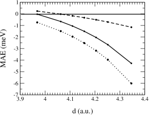
Figure 11: Magnetic anisotropy energy (MAE) $E_{100}-E_{001}$ as a function of the interatomic distance of a triangular iron cluster from HF1 (full line), HF3 (dashed line) and HF3+OPA (dotted line) models. Note that the MAE curve $E_{010}-E_{001}$ would be undistinguishable from $E_{100}-E_{001}$ since there is almost no in-plane anisotropy.

Since non-collinear magnetism is always a possible issue in clusters, we have checked for the five clusters that the most stable spin configuration is the ferromagnetic collinear one. To this aim we have initialized our calculation by arbitrary non-collinear magnetic configurations and iterated until convergency. In most cases a ferromagnetic collinear configuration is obtained. However, depending on the initial conditions, several collinear and non-collinear antiferromagnetic-like configurations, (i.e., with zero total magnetic moment) are sometimes found, but their energy is always above the ferromagnetic one. Interestingly when the calculation converges towards the ferromagnetic configuration the self-consistent scheme proceeds as follows: in the first iterations the magnetic moments tend to align along a given direction (depending on the initial condition), then once the moments are almost aligned it takes a long time for the system to converge towards the easy axis. For all clusters we were able to find the easy axis by this procedure except for the cuboctahedron. In fact depending on the initial conditions the calculation sometimes converges towards the $S$ (apex) configuration, sometimes towards the $F_{3}$ (center of triangular facet), meaning that the total energy possesses several local minima.

triangle
	MAE=$E_{\bm{u}}-E_{001}$ (meV)
$\bm{u}\rightarrow$	$(100)$	$(010)$
HF1	-1.264	-1.270
HF3	-0.246	-0.246
HF3+OPA	-2.225	-2.253
square
	MAE=$E_{\bm{u}}-E_{001}$
$\bm{u}\rightarrow$	(100)	$(110)$
HF1	8.911	15.245
HF3	5.378	6.3190
HF3+OPA	20.560	26.346
octahedron
	MAE=$E_{\bm{u}}-E_{001}$ (meV)
$\bm{u}\rightarrow$	$(100)$
HF1	-0.004
HF3	-0.001
HF3+OPA	0.021
cuboctahedron
	MAE=$E_{\bm{u}}-E_{F_{4}}$ (meV)
$\bm{u}\rightarrow$	$S$	$F_{3}$
HF1	-1.676	-2.208
HF3	-0.331	-0.441
HF3+OPA	-0.358	-0.359
icosahedron
	MAE=$E_{\bm{u}}-E_{S}$ (meV)
$\bm{u}\rightarrow$	$F_{3}$
HF1	0.114
HF3	0.020
HF3+OPA	-0.020

Table 3: Magnetic anisotropy energy in meV for various iron clusters from HF1, HF3 and HF3+OPA models calculated at the equilibrium interatomic distance. For the cuboctahedron and the icosahedron the direction $\bm{u}$ is determined by the vector joining the central atom to an apex (S) and to the centers of a triangular facet ($F_{3}$) or a square facet ($F_{4}$)

Let us now consider the orbital moment. The results of our calculations are presented in Tables 4 and 5. It is seen that the orbital moment is very sensitive to the magnetization orientation as at surfaces and in the monatomic wire. Furthermore two structurally equivalent atoms now become ”magnetically” inequivalent and can bear orbital moments that differ by a factor of more than two. For instance in a cuboctahedron with a magnetization pointing towards the center of the square facet $F_{4}$ the 8 atoms forming the upper and lower square facet (with respect to the magnetization axis) have an orbital moment about twice smaller than that of the four other outershell atoms whatever the model. The orbital moment of the central atom is close to the bulk bcc value. In contrast the icosahedron shows a more equally distributed orbital moment and the orbital moment on the central atom is significantly larger than in the bulk. Moreover the difference between the values obtained from the various hamiltonians is much less pronounced.

Finally, as expected and contrary to the spin moment, the type of hamiltonian has most often a strong influence on the numerical value of the orbital moment. We find that HF3 systematically predicts the smallest ones. However, contrary to the case of MAE, there is now a fairly good agreement between HF1 and HF3+OPA. It should be pointed out that when two magnetic orientations have almost the same energy the total orbital moment in these two directions are almost identical. This can be verified from Tables 3 and 4 in the case of the $(100)$ and $(010)$ directions of the triangle. One should however not conclude that in the HF1 model the MAE is simply related to the orbital moment. Indeed, with this model, the easy axis of the triangle corresponds to the highest orbital moment but this is not true for the square.

triangle
	$\langle L_{Z}\rangle$ ($\mu_{B}$)
$\bm{Z}\rightarrow$	$(001)$	$(100)$	$(010)$
HF1	0.133 (3)	0.177 (2)	0.216 (2)
		0.236 (1)	0.159 (1)
HF3	0.090 (3)	0.112 (2)	0.129 (2)
		0.138 (1)	0.104 (1)
HF3+OPA	0.130 (3)	0.189 (2)	0.229 (2)
		0.238 (1)	0.159 (1)
square
	$\langle L_{Z}\rangle$ ($\mu_{B}$)
$\bm{Z}\rightarrow$	$(001)$	$(100)$	$(110)$
HF1	0.325 (4)	0.337 (4)	0.234 (2)
			0.259 (2)
HF3	0.255 (4)	0.164 (4)	0.133 (2)
			0.142 (2)
HF3+OPA	0.487 (4)	0.362 (4)	0.249 (2)
			0.270 (2)
octahedron
	$\langle L_{Z}\rangle$ ($\mu_{B}$)
$\bm{Z}\rightarrow$	$(001)$	$(100)$
HF1	0.124 (4)	0.128 (4)
	0.133 (2)	0.124 (2)
HF3	0.087 (4)	0.094 (4)
	0.101 (2)	0.087 (2)
HF3+OPA	0.128 (4)	0.140 (4)
	0.153 (2)	0.128 (2)

Table 4: Local orbital moments of iron triangular, square and octahedral clusters for various magnetization orientations $Z$(see Fig. 9), from HF1, HF3 and HF3+OPA hamiltonians at the equilibrium distance. The number of sites having the same orbital moment for symmetry reasons is given in parenthesis. In the case of the $(110)$ direction of the square the largest value corresponds to the diagonal of the square perpendicular to the magnetization.

cuboctahedron
	$\langle L_{Z}\rangle$ ($\mu_{B}$)
$\bm{Z}\rightarrow$	$F_{4}$	$S$	$F_{3}$
HF1	0.098 (1)	0.101 (1)	0.102 (1)
	0.156 (8)	0.246 (8)	$\approx$0.23 (12)
	0.304 (4)	0.153 (2)
		0.182 (2)
HF3	0.063 (1)	0.063 (1)	0.064 (1)
	0.098 (8)	0.143 (8)	$\approx$0.13 (12)
	0.182 (4)	0.095 (2)
		0.104 (2)
HF3+OPA	0.103 (1)	0.105 (1)	0.105 (1)
	0.158 (8)	0.255 (8)	$\approx$0.23 (12)
	0.321 (4)	0.162 (2)
		0.179 (2)
icosahedron
	$\langle L_{Z}\rangle$ ($\mu_{B}$)
$\bm{Z}\rightarrow$	$S$	$F_{3}$
HF1	0.202 (1)	0.202 (1)
	0.317 (10)	$\approx$0.32(12)
	0.304 (2)
HF3	0.207 (1)	0.207 (1)
	0.222 (10)	$\approx$0.22(12)
	0.210 (2)
HF3+OPA	0.271 (1)	0.271 (1)
	0.312 (10)	$\approx$0.28 (6)
	0.268 (2)	$\approx$0.32 (6)

Table 5: Local orbital moments of iron for cuboctahedral and icosahedral clusters for various magnetization orientations $Z$ determined by the vector joining the central atom to an apex (S) and the centers of a triangular facet ($F_{3}$) or of a square facet ($F_{4}$), from HF1, HF3 and HF3+OPA hamiltonians at the equilibrium inter-atomic distance. The number of sites having the same orbital moment for symmetry reasons is given in parenthesis, except for the direction denoted as $F_{3}$ for which the orbital moments are very similar on all the external atoms. In the case of the $S$ direction of the cuboctahedron the smallest orbital moment in the outershell corresponds to the two atoms with a binding direction parallel to the magnetization.

VII Conclusion

In conclusion, this work presents an extended study of orbital polarization effects on the magnetic properties of iron systems with various dimensionalities using a $s,p,d,$ tight-binding hamiltonian with spin-orbit coupling and $dd$ electronic interactions treated in the Hartree-Fock scheme at different levels of approximations. The results obtained from the full Hartree-Fock interaction hamiltonian HF1, i.e., involving all matrix elements of the Coulomb interactions with their exact orbital dependence as a function of the three Racah parameters, have been systematically compared with those of simplified hamiltonians including or not the orbital polarization ansatz (OPA). As expected it is found that the one-parameter Stoner-like hamiltonian HF3 which, similarly to the L(S)DA approach, neglects the orbital dependence of Coulomb interactions, leads to reasonable values of the spin moment but largely underestimates the orbital moment and the magnetocrystalline anisotropy energy (MAE). The two-parameter (U, J) HF2 model, in which three and four orbital matrix elements are neglected and those with two different orbitals are averaged in the cubic harmonics basis, leads practically to the same results as the Stoner-like hamiltonian, at least when the spin moment is saturated. In both these simplified hamiltonians the addition of the OPA, which is not really justified on theoretical grounds, gives largely improved values of the orbital moment but is much less reliable for the MAE, at least in clusters or when the spin moment is not saturated. With the full interaction hamiltonian HF1, the orbital moment and the MAE attain numerical values of the same order of magnitude as those measured experimentally although larger, which is not surprising since the experiments have been performed on supported clusters or chains.

Furthermore HF1 is fully rotationally invariant as well in spatial and in spin coordinates. The influence of spin-flip terms is rather weak in the case of iron but is expected to increase drastically with the spin-orbit coupling parameter. This could be important for platinum which has been shown to be magnetic in monatomic wires Delin04 . Finally it should be emphasized that it is not much more computer demanding to deal with the HF1 model. It is thus of prime importance to work with this model for the study of orbital magnetism and MAE in low dimensional systems either in a realistic $s,p,d,$ tight-binding basis set or to implement it in ab-initio codes of the LDA+U type.

Appendix A The relation between HF1 and HF3 interaction hamiltonians

In this appendix, we show, using the real $d$ orbital basis set, that the Stoner-like hamiltonian HF3 can be obtained from the full Hartree-Fock interaction hamiltonian $H_{\text{int},dd}^{\text{HF1}}$ with the following approximations:

i) The intra-atomic matrix density is assumed to be diagonal with respect to both orbital and spin indices.

ii) For each spin and at each site the exact population of the $\nu\sigma$ spin-orbital is replaced by its average value, i.e., $n_{i\sigma}=1/5\sum_{\nu}n_{i\nu\sigma}$ then the matrix elements of the approximate electronic interaction hamiltonian become:

$$H_{i\lambda\sigma,i\mu\sigma}=n_{i\sigma}\sum_{\nu}(U_{\nu\lambda\nu\mu}-U_{\nu\lambda\mu\nu})+n_{i-\sigma}\sum_{\nu}U_{\nu\lambda\nu\mu}$$ (13)

It can be shown Griffith61 that the matrix elements $U_{\lambda\mu\nu\eta}$ vanish when three indices are equal and that the elements involving three different orbitals obey the relations $\sum_{\nu}U_{\nu\lambda\nu\mu}=0$ and $\sum_{\nu}U_{\nu\lambda\mu\nu}=0$. Consequently the approximate hamiltonian is diagonal and:

$$H_{i\lambda\sigma,i\lambda\sigma}=n_{i\sigma}\sum_{\nu}(U_{\nu\lambda\nu\lambda}-U_{\nu\lambda\lambda\nu})+n_{i-\sigma}\sum_{\nu}U_{\nu\lambda\nu\lambda}$$ (14)

By replacing $n_{i\sigma}$ by $(N_{i,d}+\sigma M_{i,d})/10$ we find:

$$H_{i\lambda\sigma,i\lambda\sigma}=\sum_{\nu}(U_{\nu\lambda\nu\lambda}-\frac{U_{\nu\lambda\lambda\nu}}{2})\frac{N_{i,d}}{5}-\sigma\sum_{\nu}U_{\nu\lambda\lambda\nu}\frac{M_{i,d}}{10}$$ (15)

Carrying out the summations over $\nu$ leads to:

$$H_{i\lambda\sigma,i\lambda\sigma}=\frac{9U-2J}{10}N_{i,d}-\frac{\sigma}{2}(\frac{U+6J}{5})M_{i,d}$$ (16)

which are the matrix elements of the electronic interaction hamiltonian in the HF3 model.

Appendix B The penalty functions

The usual way to implement constraints in a variational problem is to use a Lagrange-multiplier formalism. For example the normalization constraint of the wave functions leads to the eigenvalue problem, the Lagrange-multiplier being the eigenvalues. However this approach is not always very well suited to more general constraints. A very useful approach is to add a supplementary term to the total energy functionGebauerPhD ; Cohen04 . This term called penalty function is equal to zero when the constraint is fulfilled and large and positive when it is not. In the present work we have used a local charge neutrality (LCN) penalty $E^{\text{pen}}_{\text{LCN}}$ and a $\theta$ angle penalty $E^{\text{pen}}_{\text{ang}}$. We have taken the following forms for these penalty functions:

$$E^{\text{pen}}_{\text{LCN}}=\lambda^{\text{pen}}_{\text{LCN}}\sum_{i}(\Delta q_{i})^{2}$$ (17)

and:

$$E^{\text{pen}}_{\text{ang}}=\lambda^{\text{pen}}_{\text{ang}}\sum_{i}(\cos\theta_{i}-\cos\theta_{i0})^{2}$$ (18)

$\Delta q_{i}=q_{i}-q_{0}$ where $q_{i}$ is the Mulliken charge of site $i$, $q_{0}$ the valence charge and $\lambda^{\text{pen}}_{\text{LCN}}$ the penalization factor which must be taken large enough to ensure local charge neutrality; $\theta_{i}$ is the local magnetization angle on atom $i$ and $\theta_{i0}$ the angle that one wants to impose. Using the expression of $q_{i}$ and $\cos\theta_{i}=M_{iz}/\sqrt{M_{ix}^{2}+M_{iy}^{2}+M_{iz}^{2}}$ in terms of the tight-binding expansion coefficients of the wave functions, the calculation of the derivative of the penalized total energy with respect to these expansion coefficients leads to an eigenvalue problem where the hamiltonian is now modified by an additional ”renormalizing” term which matrix elements reads:

$$\lambda^{\text{pen}}_{\text{LCN}}(\Delta q_{i}+\Delta q_{j})\sigma_{0}S_{ij}^{\lambda\mu}$$

and

$$-\lambda^{\text{pen}}_{\text{ang}}(\bm{B}^{\text{pen}}_{i}+\bm{B}^{\text{pen}}_{j}).\bm{\sigma}S_{ij}^{\lambda\mu}$$

in the case of LCN and angle penalization, respectively, where $\sigma_{0}$ is the identity matrix and $\bm{\sigma}$ the Pauli matrix vectors. $\bm{B}^{\text{pen}}_{i}$ is an effective constraining magnetic field that exerts a torque to bring the magnetization along the $\theta_{i0}$ axis which expression is:

$$\bm{B}^{\text{pen}}_{i}=\lambda^{\text{pen}}_{\text{ang}}\frac{(\cos\theta_{i}-\cos\theta_{i0})}{(M_{ix}^{2}+M_{iy}^{2}+M_{iz}^{2})^{3/2}}\left(\begin{array}[]{c}M_{ix}M_{iz}\\ M_{iy}M_{iz}\\ -M_{ix}^{2}-M_{iy}^{2}\end{array}\right)$$ (19)

In practice $\lambda^{\text{pen}}_{\text{LCN}}=2.5$eV and $\lambda^{\text{pen}}_{\text{ang}}=1$eV ensure charge transfers below 0.1 electron per atom and deviations from the angle $\theta_{i0}$ smaller than $0.1^{\circ}$.

The modified eigenvalue problem has to be solved iteratively until convergence of the Mulliken charges (and total energy). Finally it should be noted that if one writes the total energy as a sum of the occupied eigenvalues, one should not forget to subtract an additional double counting term arising from the penalization function.

References

- (1) A.J. Cox, J.G. Louderback, S.E. Apsel, and L.A. Bloomfield, Phys. Rev. B 49 12295 (1994).
- (2) R. Guirado-López, D. Spanjaard, and M.C. Desjonquères, Phys. Rev. B 57, 6305 (1998).
- (3) R. Guirado-López, D. Spanjaard, M.C. Desjonquères, and A.M. Oles, Euro. Phys. J. B 3, 437 (1998).
- (4) C. Barreteau, R. Guirado-López, D. Spanjaard, M.C. Desjonquères, and A.M. Oleś, Phys. Rev. B 61, 7781 (2000).
- (5) P. Gambardella et al., Nature 416, 301 (2002).
- (6) P. Gambardella et al., Science 300, 1130 (2003).
- (7) K.W. Edmonds, C. Binns, S.H. Baker, M.J. Maher, S.C. Thornton, O. Tjernberg, and N.B. Brookes, J. Mag. Magn. Mater. 200, 25 (2000).
- (8) C. Binns, S.H. Baker, M.J. Maher, S.C. Thornton, S. Louch, S.S. Dhesi, and N.B. Brookes, Euro. Phys. J. D 16, 189 (2001).
- (9) G. Autès, C. Barreteau, D. Spanjaard and M.C. Desjonquères, J. Phys.:Condens. Matter 18, 6785 (2006)
- (10) Yuannan Xie and John A. Blackman, J. Phys.:Condens. Matter 16, 3163 (2004).
- (11) O. Eriksson, M.S.S. Brooks and B. Johansson, Phys. Rev.B 41, 9087 (1990)
- (12) G. Nicolas, J. Dorantes-Davilá, and G.M. Pastor, Comp. Mat. Sci. 35, 292 (2006).
- (13) V.I. Anisimov, I.V. Solovyev, M.A. Korotin, M.T. Czyzyk and G.A. Sawatzky, Phys. Rev.B 48, 16929 (1993)
- (14) M. Wierzbowska, A. Delin, and E. Tosatti, Phys. Rev. B 72, 035439 (2005).
- (15) A.I. Liechstenstein, V.I. Anisimov, and J. Zaanen, Phys. Rev. B 52, R5467 (1995).
- (16) A.B. Shick, F. Máca, and P.M. Oppener, Phys. Rev. B 69, 212410 (2004).
- (17) M.C. Desjonquères, C. Barreteau, G. Autès and D. Spanjaard, Eur. Phys. J.B 55, 23 (2007).
- (18) I.V. Solovyev, A.I. Liechstenstein, and K. Terakura, Phys. Rev. Lett. 80, 5758 (1998).
- (19) J.C. Slater and G.F. Koster, Phys. Rev. 94, 1498 (1954)
- (20) M.J. Mehl and D.A. Papaconstantopoulos, Phys. Rev.B 54, 4519 (1996)
- (21) http://cst-www.nrl.navy.mil/bind/
- (22) J.S. Griffith, The Theory of Transition Metal Ions (Cambridge University Press, London, 1961)
- (23) M.T. Czyzyk and G.A. Sawatzky, Phys. Rev.B 49, 14211 (1994)
- (24) I.V. Solovyev, Phys. Rev. Lett. 95, 267205 (2005)
- (25) D. Bonnenberg, K.A. Hempel and H.P.J. Wijn, Numerical Data and Functional Relationship in Science and Technology Landolt-Brnstein New Series Group 3 19 Part a) Ed.H.P.J. Wijn (Springer, Berlin, 1986)
- (26) P. Bruno, Phys. Rev.B 39, 865 (1989)
- (27) S. Datta Electronic Transport in Mesoscopic Systems. Cambridge University Press.
- (28) M. Viret, M. Gabureac, F. Ott, C. Fermon, C. Barreteau G. Autès, and R. Guirado-López, Eur. Phys. J. B 51 1 (2006).
- (29) C. Barreteau, M.C. Desjonquères and D. Spanjaard, Eur. Phys. Journ. D 11 395 (2000)
- (30) A. Delin, and E. Tosatti, Surf. Sci 566-568, 262 (2004)
- (31) R. Gebauer PhD Thesis 1999, Ecole Normale Supérieure de Lyon.
- (32) R.E. Cohen and S. Mukherjee, Physics of the Earth and Planetary Interiors 143-144, 445 (2004)