Solvation Effects on Free Energy Surface of Polyalanine

Gökhan Gökoğlu ggokoglu@hacettepe.edu.tr Hacettepe University, Department of Physics Engineering , Beytepe, 06800 Ankara, Turkey Handan Arkin Olğar handan@hacettepe.edu.tr Hacettepe University, Department of Physics Engineering , Beytepe, 06800 Ankara, Turkey Ethem Aktürk eakturk@hacettepe.edu.tr Hacettepe University, Department of Physics Engineering , Beytepe, 06800 Ankara, Turkey Tarik Çelik tcelik@hacettepe.edu.tr Hacettepe University, Department of Physics Engineering , Beytepe, 06800 Ankara, Turkey

Abstract

We have simulated 10-residue polyalanine chain by multicanonical method to visualize the 3D topographic picture of the free energy landscape over the whole range of temperatures, hence to show the funnel along the folding pathway exhaustively. We have simulated and compared the system in vacuo and in solvent, and examined the changes in the free energy landscape due to the solvent effects, which are taken into account by commonly used model Accessible Surface Area.

Keywords: Free energy funnel, solvation effects, polyalanine.

pacs:

02.70.Uu Applications of Monte Carlo Methods, 05.10.-a Computational Methods in Statistical Physics and Nonlinear Dynamics, 82.20.Wt Computational Modelling Simulation.

I Introduction

The configuration space of proteins presents a complex energy profile consisting of tremendous number of local minima, barriers, attraction basins and further topological features. The problem of protein folding entails the study of a non-trivial dynamics along pathways embedded in a rugged energy landscape. The topology of the landscape characterizes the folding kinetics through the existence of folding pathway.

The topography of the energy landscape, especially near the global minimum, is of particular importance, because the potential energy surface defines the behavior of the system JBPW . However, the entropic effects play a major role in the folding process, and instead of potential energy, the landscape of the free energy surface better be examined. The essence of a funnel structure of free energy at some fixed temperatures has been shown by Hansmann and Onuchic HaOn99 . A visualization of the whole rugged free energy landscape covering the entire temperature range would lead to clear indications of the equilibrium conformations of proteins as a function of the temperature and provide a detailed picture of the folding pathway.

On the other hand, it is vital in simulations to mimic the effects of the environment which change the topology of the free energy surface to a large extent, hence alter the phase transition behaviour of the system. The solution effects can be included by incorporating the Accessible Surface Area (ASA), in which model the solvation energy term is proportional to accessible surface area of the peptide.

In this study, our aim is to obtain a 3D topographic picture of free energy surface covering the whole temperature range, display the funnel along the folding pathway and examine how the solution effects alter the free energy landscape. Such a goal can be achieved within the multicanonical ensemble approach HATC .

The conventional simulation methods are not effective because the system becomes trapped for long simulation time in a potential well. The trapping problem of the Monte Carlo and Molecular Dynamics methods can be alleviated to a large extent, by the Multicanonical MC method (MUCA) BeCe92 ; Be99 , which was applied initially to lattice spin models and its relevance for complex systems was first noticed in Ref. BeCe92 . Application of the multicanonical approach to peptides was pioneered by Hansmann and Okamoto HaOk93 and followed by others HaSc94 ; simulations of protein folding with MUCA and related generalized ensemble methods are reviewed in Refs. HaOk99rev and Ok00rev .

The multicanonical ensemble based on a probability function in which the different energies are equally probable. However, implementation of MUCA is not straightforward because the density of states $n(E)$ is unknown a priori. The weights $w(E)\sim 1/n(E)$ are calculated in the first stage of simulation process by an iterative procedure. The iterative procedure is followed by a long production run based on the fixed $w$ ’s where equilibrium configurations are sampled. Re-weighting techniques (see Ferrenberg and Swendsen FeSw88 and literature given in their second reference) enable one to obtain Boltzmann averages of various thermodynamic properties over a large range of temperatures.

By setting up a one-dimensional random walk in energy space, the multicanonical simulation provides sampling of all available energies and enables one to study the thermodynamical aspects of the system at a wide range of temperature from a single production run. In this work, we will exploit the multicanonical ensemble to investigate and compare the free energy landscape of the 10-residue polyalanine chain in vacuo and in solvent.

II Methods

ECEPP (Empirical Conformational Energies for Proteins and Polipeptides) force field, one of the most commonly used all atom force field was used in simulations. This force field composed of four potential energy terms; electrostatic, hydrogen bond, Lennard-Jones and torsion energy term.

$\displaystyle E_{ECEPP/2}$	$\displaystyle=$	$\displaystyle E_{C}+E_{LJ}+E_{HB}+E_{tor},$	(1)
$\displaystyle E_{C}$	$\displaystyle=$	$\displaystyle\sum_{(i,j)}\frac{332q_{i}q_{j}}{\epsilon r_{ij}},$	(2)
$\displaystyle E_{LJ}$	$\displaystyle=$	$\displaystyle\sum_{(i,j)}\left(\frac{A_{ij}}{r^{12}_{ij}}-\frac{B_{ij}}{r^{6}_{ij}}\right),$	(3)
$\displaystyle E_{HB}$	$\displaystyle=$	$\displaystyle\sum_{(i,j)}\left(\frac{C_{ij}}{r^{12}_{ij}}-\frac{D_{ij}}{r^{10}_{ij}}\right),$	(4)
$\displaystyle E_{tor}$	$\displaystyle=$	$\displaystyle\sum_{l}U_{l}\left(1\pm\cos(n_{l}\chi_{l})\right).$	(5)

Here, $r_{ij}$ (in Å) is the distance between the atoms $i$ and $j$ , $\chi_{l}$ is the torsion angle for the chemical bond $l$ and $n_{l}$ characterizes its symmetry. The force field parameters $q_{i},A_{ij},B_{ij},C_{ij},D_{ij},U_{l}$ were calculated from crystal structures. The dielectricity constant is set to $\varepsilon=2$ , its common value in ECEPP calculations. ECEPP force field is based on rigid geometry that means bond lengths and bond angles are constant. The backbone torsion angles $\phi$ , $\psi$ and the side chain torsion angle $\chi$ are the degrees of freedom of the system. $\omega$ torsion angle was fixed in trans position that $\omega$ = $180^{\circ}$ . Solvation energy term is Ooi ,

E_{solv}=\sum_{i}\sigma_{i}A_{i}~{},

(6)

where $A_{i}$ is the solvent accessible surface area of the $i^{th}$ atom for a definite conformation, and $\sigma_{i}$ the solvation parameter for the atom $i$ . The total potential energy of the molecule is then given by

E_{tot}=E_{ECEPP}+E_{solv}

(7)

This potential energy is implemented into the software package FANTOM FANTOM .

The order parameter chosen for the system is the normalized helicity $q$ , which is defined as HaOk99 ,

q=\frac{n_{H}}{N-2}

(8)

where $n_{H}$ is the number of residues that conforms to $\alpha$ -helix state defined in the angle range for $\phi$ $(-70\pm 20^{\circ})$ and for $\psi$ $(-37\pm 20^{\circ})$ , $N$ is the total length of the chain. End residues are more flexible than others and was not taken into account. This definition guarantees the q value between $0$ and $1$ .

Helmholtz free energy of the system was calculated by the formula

F(q,T)=-RT\log P(q)

(9)

where $P(q)$ is the probability that the system has an order parameter value $q$ at a fixed temperature $T$ and $R$ is the gas constant. This free energy is not normalized to be expressed in unit kcal/mol, however it gives a qualitative view of free energy surface.

We first carried out canonical (i.e., constant $T$ ) MC simulations at relatively high temperatures and MUCA test runs which enabled us to determine the required energy ranges. The energy range was divided into 40 bins of $1\,$ kcal/mol each, covering the range $[-10,30]\,$ kcal/mol for vacuo and 25 bins of $1\,$ kcal/mol each, covering the range $[-23,2]\,$ kcal/mol for solvent. At each update step, a trial conformation was obtained by changing one dihedral angle at random within the range [ $-180^{\rm o};180^{\rm o}]$ , followed by the Metropolis test and an update of the suitable histogram. The dihedral angles were always visited in a predefined (sequential) order; a cycle of $N$ MC steps ( $N$ =30) is called a sweep. The weights were built after $150$ recursions during a long single simulation, where the multicanonic parameters were iterated every 5000 sweeps. Then we performed full simulation of two million sweeps, which cover the temperature region up to $T_{\max}=600\,$ K reliably.

III Results and Discussion

Polyalanine is an important model system to study specially the backbone behaviour in polypeptide systems with small side chains, so that a great deal of theoretical works focus on it. The major goal of these studies is to determine the stable conformation and to investigate the structural properties of the system. The success of simulation studies strongly depends how well the nature environment of the polypeptide system was described. Hence the solvation effects must be included in simulation otherwise the results does not reflect the physical reality.

Free energy calculations in polypeptide systems in a temperature range is not straightforward and generally the potential energy is considered. However, the stable conformation of the system corresponds to the global minimum of the free energy rather than the potential energy, so that entropic contributions are taken into account.

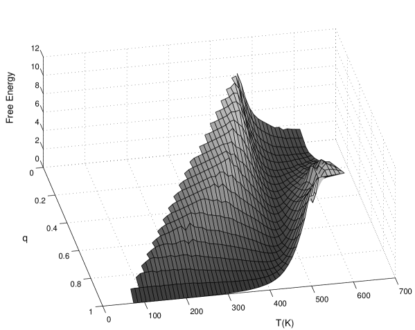
By utilizing the multicanonical technique, we have obtained 3D topographic picture of the free energy surface for 10-residue polyalanine chain in vacuo over whole temperatures and plotted vs. the order parameter in Fig.1a. It can be seen from the figure that there is no data for some $q(T)$ values, which means no histograms detected in that region and these states can be regarded as non-accessible. The free energy surface displays an apparent valley structure, which clearly pictures the existing funnel towards the state of global energy minimum (GEM). Free energy surface has two wings divided by a valley along which the free energy is lower than other parts of the surface. The states with lower free energy lie in the riverbed along the valley and serves one to visualize the folding pathway. From high temperatures to lower ones, the system will follow that valley from one corner of the $q-T$ plane to other and will make a transition from a disordered state to highly ordered state that is the well known helix-coil transition. The ordered state $(q=1)$ has the minimum free energy which is the stable conformation for the systems under study. Global energy minima found in our simulations of the system in vacuo and in solvent are $E=-9.9722$ kcal/mol and $E=-22.8079$ kcal/mol, respectively, both conform to a stable $\alpha$ -helix structure. Our results supports that of Scholtz et al. suggesting that longer polyalanine chains form stable $\alpha$ -helices in water Scholtz . The system in vacuo has a big tendency to $\alpha$ - helical conformations that the system is in exact helical state up to temperatures $400K$ . It is known that polyalanine has an intrinsic tendency to $\alpha$ - helical conformations.

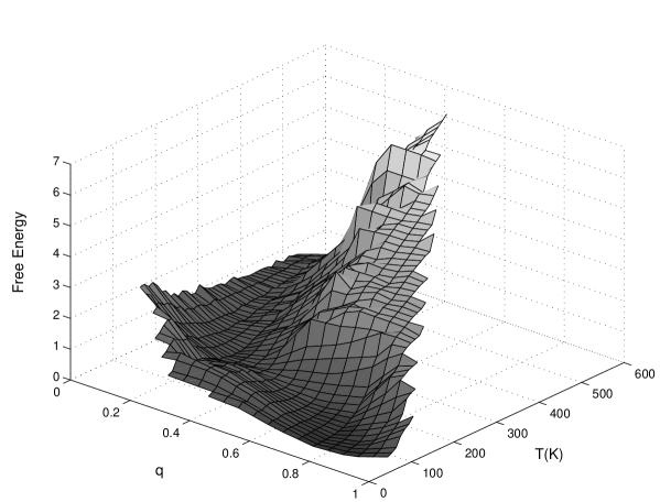
The free energy surface of the 10-residue polyalanine chain in solvent is displayed in Fig.1b. If we compare the free energy surfaces of the same system in vacuo and in solvent, the valley is quite distorted, one of the wings is almost disappeared and the whole picture is pulled down to lower temperatures. In both figures, the side with lower free energy is more probable hence the system with solvent is in highly disordered state at temperatures higher than $150K$ . The disordered states are still probable in solvent with low $q$ value at temperatures as low as $100K$ .

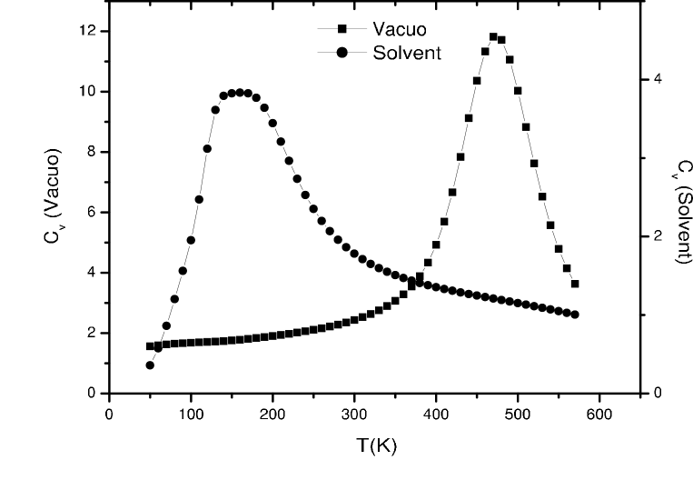
Drastic changes in free energy surface by putting the system in solvent can be attributed to that the solvent used in simulations is water which is a good solvent specially for polyalanine chain. Due to large increase in entropy, free energy surface becomes much altered in solvent. This massive effect can also be seen in Fig. 2, where the phase transition temperature are $490K$ and $170K$ for the systems vacuo and solvent, respectively. Decrease in specific heat for the system in solvent is an expected result for peptides.

In Fig.3, free energy is shown as a function of the order parameter at distinct temperatures for the system in vacuo. At critical temperature $T_{c}=490K$ free energy makes a deeper valley than other temperatures and the whole sequence of fixed temperature plots mimics a smooth phase transition. But it must be remembered that, in small systems, a first order phase transition may be seen as if it is continuous.

IV Conclusion

In conclusion, we have simulated the 10-residue polyalanine chain by utilizing multicanonical ensemble approach and investigated the structure of rugged free energy landscape in configurational space. We were able to display the distribution of all conformations in the configuration space at all temperatures from a single simulation. From the topographic picture obtained, one can visualize the structure of the folding pathway and the changes due to solution effects. Such a visualization of the rugged energy landscape would certainly be helpful in another aspect, namely in designing algorithms for efficient sampling of conformational space.

Acknowledgments:
This work is supported by Hacettepe University Scientific Research Fund through project No: 02.02.602.010.

References

(1) J.D. Bryngelson, P.G. Wolynes, Proc. Natl. Acad. Sci. 84, 7524 (1987).
(2) U.H.E. Hansmann, Y. Okamoto, J.N. Onuchic, Proteins 34, 472 (1999) ; U.H.E. Hansmann, J.N. Onuchic, J. Chem. Phys. 115, 1601 (2001).
(3) H. Arkın, T. Çelik, Int. J. Mod. Phys. C 14, 113 (2003).
(4) B.A. Berg, T. Çelik, Phys. Rev. Lett. 69, 2292 (1992).
(5) B.A. Berg, Fields Institute Communications 28, 1 (1992).
(6) U.H.E. Hansmann, Y. Okamoto, J. Comp. Chem. 14, 1333 (1993).
(7) M.H. Hao, H.A. Scheraga, J. Phys. Chem. 98, 4940 (1994) ; J. Phys. Chem. 98, 9882 (1994); A. Kolinski, W. Galazka, J. Skolnick, Proteins 26, 271 (1996); J. Higo, N. Nakajima, H. Shirai, A. Kidera, H. Nakamura, J. Comp. Chem. 18, 2086 (1997).
(8) U.H.E. Hansmann, Y. Okamoto, Ann. Rev. Comp. Physics 5, 129 (1999).
(9) A. Mitsutake, Y. Sugita, Y. Okamoto, Biopolymers (Peptide Science) 60, 96 (2001).
(10) A.M. Ferrenberg, R.H. Swendsen, Phys. Rev. Lett. 61, 2635 (1988); Ibid 63, 1658 (1989).
(11) T. Ooi, M. Obatake, G. Nemethy, H.A. Scheraga, Proc. Natl. Acad. Sci. 8, 3086 (1987).
(12) B. von Freyberg, T. Schaumann, W. Braun, FANTOM User’s Manual and Instructions: ETH Zürich, Zürich, 1993 ; B. von Freyberg, W. Braun, J. Comp. Chem. 14, 510 (1993).
(13) U.H.E. Hansmann, Y. Okamoto, J. Chem. Phys. 110, 1267 (1999).
(14) J.M. Scholtz, H. Qian, E.J. York, J.M. Stewart, R.L. Baldwin, Biopolymers 31, 1463 (1991).

Figure Captions:

Fig. 1: Free energy surface of polyalanine in vacuo (upper)and in solvent (lower). The funnel structure is exhaustively displayed.
Fig. 2: Specific heat as a function of the temperature for 10-residue polyalanine chain in vacuo and in solvent.
Fig. 3: Free energy as a function of the order parameter at $T=380,460,490$ and $520K$ .

Refer to caption — Figure 1: Free energy surface of polyalanine in vacuo (upper) and in solvent (lower). The funnel structure is exhaustively displayed.