New boundary conditions for granular fluids
Abstract
We present experimental evidence, which contradicts the the standard boundary conditions used in continuum theories of non-cohesive granular flows for the velocity normal to a boundary , where points into the fluid. We propose and experimentally verify a new boundary condition for , based on the observation that the boundary cannot exert a tension force on the fluid. The new boundary condition is if else , where P is the pressure tensor. This is the analog of cavitation in ordinary fluids, but due the lack of attractive forces and dissipation it occurs frequently in granular flows.
pacs:
45.70.-n, 51.30.+j, 51.10.+y, 64.70.HzI Introduction
Granular materials, collections of particles which dissipate energy through inter-particle interactions have tremendous technological importance and numerous applications to natural systems. They also represent a serious challenge to statistical and continuum modeling, due to the small number of particles and dissipation. A fundamental understanding of granular systems, comparable to our current understanding of fluids and solids, does not exist today Kadanoff (1999) but would have far reaching implications across many industries.
The idealized granular system, a collection of identical inelastic hard spheres, is a laboratory scale analog of the canonical system in kinetic theory — the elastic hard sphere gas. Using this analogy, an inelastic version of the Boltzmann-Enskog equation have be derived Chapman and Cowling (1970); Jenkins and Richman (1985a) as well as an inelastic version of continuum equations for mass, momentum, and energy balance Chapman and Cowling (1970); Jenkins and Richman (1985a); Goldshtein and Shapiro (1995); Sela et al. (1996); Brey et al. (1996); Santos et al. (1998); van Noije et al. (1998) nearly identical to the Navier-Stokes equations. These type of equations can produce a quantitative description of dilute granular flows with an accuracy of 1% Rericha et al. (2002). Boundary conditions for velocity and granular temperature have been derived to complete these equation Jenkins and Askari (1991); Richman (1992); Jenkins (1992); Jenkins and Louge (1997), which assume that the fluid never leaves the boundary.
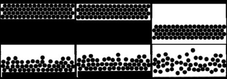
Normal fluids remain attached to boundaries due to two effects — adhesion and pressure (external and internal). External pressure is unimportant and adhesion is not present in non-cohesive granular materials leaving the internal pressure alone to hold a granular fluid to a boundary. However, if the force on the granular fluid accelerates the fluid to a velocity greater than the average root-mean-squared particle velocity (square root of the granular temperature), then the boundary and the granular fluid will separate. This is the analog of cavitation in normal fluids. While cavitation is unusual in normal fluids, low granular temperature at boundaries due to inelastic loss combined with the lack of external pressure and adhesion makes cavitation common in granular fluids (see Fig. 1). Common examples include rotating drums and vibrated layers. Many features of pattern formation in vibrated layers Melo et al. (1994) can be understood in terms of the time that the layer spends off of the plate Melo et al. (1995). It difficult to explain this dependence with models which do not allow the granular fluid to leave the boundary.
II New Boundary Condition
The standard boundary condition Jenkins and Askari (1991); Richman (1992); Jenkins (1992); Jenkins and Louge (1997) for the velocity normal to the wall is
| (1) |
for the fluid velocity u on a boundary with inward unit normal and wall velocity v. In order to enforce this condition the boundary must exert a force on the granular fluid. Because there is no attractive force between the grains and the boundary . When the force needed to maintain zero velocity is negative the boundary condition must be changed. Since the boundary force then must be zero a no stress condition is the logical choice. As the normal wall velocity will no longer be zero we must have a another condition to enforce the no particle flux condition at the boundary. Analytically more work needs to be done to understand this new condition on the flux . Numerically, we treat the density and velocity as centered in the grid and the flux is defined on the boundaries of the grid. In that case the density and velocity in the cell nearest the boundary are both non-zero, but the flux on the wall is zero (see (§ IV) for details of the flux condition). Altogether we have
| (2) |
III Experiment
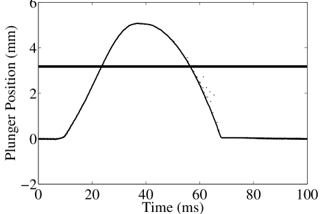
We have performed two types of experiments to elucidate the role of boundary conditions in continuum equations of motion for granular materials — free-fall and vibrated. We place (–) spherical stainless steel ball bearings of diameter mm in a container 17.5 wide by 20 tall by 1 deep as shown in Fig. 1. We define the number of rows , where 17 is the number of particles to fill an entire row in a close-packed structure. We control a thin plunger, which slides through a slot in the bottom of the cell. For the free-fall experiment [Fig. 1(top row)] the plunger pushes all of the particle to the top of the cell to start the experiment. The particles are then vibrated in order to compact them into a perfect hexagonal packing [Fig. 1(top-left)]. Then the plunger is pulled downward with an initial acceleration of , where is the acceleration of gravity. The particles are then free to fall under gravity. This process is under computer control and can be repeated many times. In the vibrated experiments [Fig. 1(bottom row)] the plunger oscillates sinusoidally, but is offset from the bottom of the container to produce a half-sine-wave excitation. The measured position of the plate is shown in Fig. 2. 94 oscillations are superimposed to show the repeatability of the drive. The excitation is characterized by the non-dimensional maximum acceleration , where is the maximum amplitude of the plunger and is the frequency. Using high-speed digital photography we measure the positions of the plunger and all of the particles in the cell with a relative accuracy of 0.2% of or approximately m at a rate of 840 Hz. We track the particles from frame to frame and assign a velocity to each one, typically per frame.
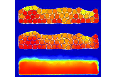
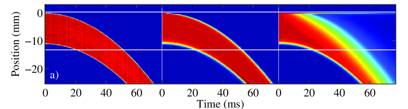
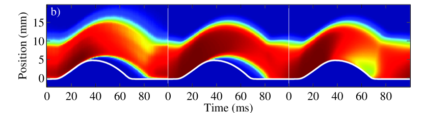
To compare with the continuum theories through our simulations (see Section IV), we must average the particle trajectories to created density, velocity, and temperature fields. We are interested in studying the flow as the grains separate from the boundary so we focus on the density fields. To create average fields we run each flow condition 90-100 times. In each frame, we construct a modified Voronoi cell around each particle and fill it with a uniform number density of 1 particle divided by the area of the cell. We modify the Voronoi cells on the border by including only the area that overlaps with a sector created by two lines both tangent to the particles edge and tangent to two other neighbors less than two particle diameters away. This is the union of the convex hull formed by all all particle pairs whose centers lie within 2 particle diameters of each other. The results of such a construction are shown in Fig. 3(top). Next, we apply a mask preserving spatial average over 2 particle diameters [Fig. 3(middle)]. The mask is formed by the union of all of the modified voronoi cells. Finally, we bin the frames according the phase of the cycle and average each bin [Fig. 3(bottom)]. From these images we have determined that the flow is uniform in the horizontal direction for both free-fall and vibrations. Therefore, to obtain one dimension density field along the vertical direction. Space-time intensity plots of these densities are shown in Fig. 4.
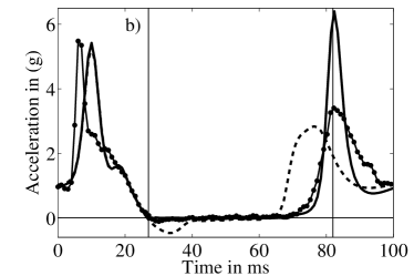
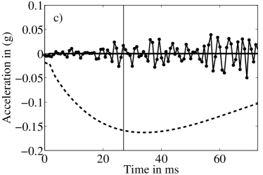
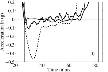
As a further quantitative comparison, we calculated the discharge rate for the free-fall case [Fig. 5(a)] and the acceleration of the center of mass minus g for all cases [Fig. 5(b–d)]. , where is the total mass of the fluid. In Fig. 5(b–d) we plot for both the free fall and the vibrating case.

IV Simulation
We numerically integrate the continuum equations for the balance of mass, momentum, and energy have been derived for two-dimensional (2D) granular flows Jenkins and Richman (1985a, b):
| (3) | |||||
| (4) | |||||
| (5) |
where is the mass density, g is the gravity vector, is the granular temperature, q is the heat flux vector, are the elements of the symmetrized velocity gradient tensor E, and is the temperature loss rate. The constitutive relations for the pressure tensor P and heat flux q are
| (6) |
and
| (7) |
where Tr denotes trace and is the unit tensor. The 2D equations close Jenkins and Richman (1985b) with the equation of state, which is the ideal gas equation of state with a term that includes dense gas and inelastic effects,
| (8) |
where is the coefficient of restitution, is the volume fraction, is the diameter of the particles, is the mass of the particles, and , where is the value of the radial distribution function at a distance of one particle diameter. We use a temperature dependent
| (9) |
This mimics the experimental evidence that goes to zero for small velocities. We use a form for developed by Torquato Torquato (1995), which is an analytical fit to molecular dynamics simulation at high and the Carnahan and Starling Carnahan and Starling (1969) geometric series approximation to the first few viral coefficients at low . We have changed the functional form of and the details of the flow change, but not the qualitative behavior. The bulk viscosity,
| (10) |
the shear viscosity,
| (11) |
the thermal conductivity,
| (12) |
and the temperature loss rate per unit volume,
| (13) |
We use a second-order-space adaptive first-order-time finite-differencing scheme to integrate these equation. We use off-center-differencing at the boundaries to maintain second-order accuracy. The code uses an adaptive time step based on a modified Courant condition combined with an empirically determined maximum and minimum time step. We used a 5x161 point - grid, with periodic boundary conditions in the direction. We use the temperature and tangential velocity boundary condition for smooth surfaces found in reference Jenkins (1992). We can alternate between our new (2) and the standard boundary conditions for the normal velocity. To maintain mass conservation we use a special differencing procedure for the mass continuity equation, which is second-order accurate for both the new and old boundary conditions and is exactly conserving. In one dimension we label the density and velocity and for to . We then define fluxes for to , and . Then the change in density at position is , where is the current time step. From these definitions it follows that and , regardless of the value of and at the boundaries. The only boundaries in the system are the actual walls. We let the free surfaces develop on there own simply as very low density regions. As the density of a gas becomes so dilute that the mean free path is comparable to the size of the container the transport equations must be modified. We define a transport cutoff at a density of
| (14) |
where is the dimensionless cutoff mean free path. At lower densities than this the viscosity and thermal conductivity are multiplied by the factor
| (15) |
For is close to unity, but as the density decreases the transport coefficients go smoothly to zero. This ad-hoc factor is used only to prevent the code from diverging at extremely low densities. In these simulations, we have varied from 10-100 and the results are almost the same except for slight deviations in the very low-density regions. This low density regime does not effect the main flow as the momentum and energy are also nearly zero unless the temperature or velocity diverge, which is prevented by this approach.
We use the following parameter for all of the simulations presented here: and . Both of these parameter effect the energy loss. If the energy loss is not great enough the separation does not occur. These values were not formally optimized, but several different value of between 0.6 and 0.9 were tried, but anything below 0.8 gave approximately the same flight-time for the vibrated case. The temperature and tangential velocity boundary conditions require two additional parameters, and , the wall coefficients of restitution and friction. These parameters only have a small effect on the flow.
For the free-fall case we solve the equation in the lab frame. To create an initial condition we set gravity upwards to push the fluid to the top of the container. Then we slowly decrease gravity to zero and then abruptly change the value of to . The results of the horizontally averaged density are shown as space-time plots in Fig. 4 for both the new and old boundary conditions. For the vibrated case we solve the problem in the reference frame of the bottom plate. We determine the acceleration of the plate from the experimentally determined position of the plate Fig. 2. The second derivative is quite noisy so the signal is convolved with a 5 ms top-hat function. The signal is then corrected so that the average acceleration is zero. The initial condition is a uniform distribution and wait for the density to reach a stable periodic state. This typically takes 5-10 oscillations. The final cycle is shown in Fig. 4 for both types of boundary conditions.
V Results
Comparing the first two columns in Fig. 4 (experiment and new boundary conditions) to the third there is a striking effect. In the free-fall experiment the zero velocity boundary condition holds the fluid to the top surface long after all of the grains in the experiment and the new boundary condition simulation have left the domain of interest. To see this in a quantitative way we look at the rate the particles pass the lower line in the figure. The result is shown in Fig. 5(a). Initially the two simulation follow more closely due to the lack of dispersion in the experiment. The dispersion in the simulation is not due to temperature, but an artifact of the truncation error in the mass conservation equations. Shortly ( ms) all three curves meet, but by ( ms) the old boundary conditions simulation begins to diverge, and from there on the behavior is radically different. As the last of the material flows from the experiment and new BC simulation there is another small lag, but the old BC simulation continues to flow for another 30 ms. Figure 5(c) shows that there is a negative acceleration induced by the old BCs. Both the experiment and the new BCs show zero acceleration throughout the time of the experiment.
In Fig. 4(b) the layer is stuck to the boundary for the old BCs. There is no clear flight time. From the layer acceleration in Fig. 5(b) we see that there is still some kind of a collision for the old BCs but it occurs earlier. Further, there is a clear region of negative acceleration, as seen in the expanded axis of Fig. 5(d) of nearly half the value of gravity. The small negative acceleration in the experiment is likely due to friction with the walls. The take off time and collision time shown by the two vertical line are the same for the experiment and the new BCs.
VI Conclusions
The new boundary conditions provide a significant improvement in simulating these flows. Separation (cavitation) is a very common situation in granular flows, and this type of boundary condition is needed to capture the basic features of the flows presented. Without this type of boundary condition many qualitative features may be missed, and there is no hope quantitative agreement. There are still a number of open question including: what should happen in corners, and how can these BCs be treated analytically? Previously we have shown that molecular dynamics (MD) simulation Bizon et al. (1998); Moon et al. (2002) are capable of quantitatively reproducing the flow in dense vibrated pattern forming system, and MD and continuum simulation can reproduce dilute flows in which granular shocks form Rericha et al. (2002). However, this work represents a first, big step in getting quantitative agreement using continuum simulations in dense vibrated pattern forming systems.
Acknowledgements.
This work is supported by The National Science Foundation, Math, Physical Sciences Department of Materials Research under the Faculty Early Career Development (CAREER) Program: DMR-0134837.References
- Kadanoff (1999) L. P. Kadanoff, Rev. Mod. Phys. 71, 435 (1999).
- Chapman and Cowling (1970) S. Chapman and T. G. Cowling, The Mathematical Theory of Non-uniform Gases (Cambridge University Press, London, 1970).
- Jenkins and Richman (1985a) J. T. Jenkins and M. W. Richman, Arch. Rat. Mech. Anal. 87, 355 (1985a).
- Goldshtein and Shapiro (1995) A. Goldshtein and M. Shapiro, J. Fluid Mech. 282, 75 (1995).
- Sela et al. (1996) N. Sela, I. Goldhirsch, and S. H. Noskowicz, Phys. Fluids 8, 2337 (1996).
- Brey et al. (1996) J. J. Brey, F. Moreno, and J. W. Duffy, Phys. Rev. E 54, 445 (1996).
- Santos et al. (1998) A. Santos, J. M. Montanero, J. W. Dufty, and J. J. Brey, Phys. Rev. E 57, 1644 (1998).
- van Noije et al. (1998) T. P. C. van Noije, M. H. Ernst, and R. Brito, Physica A 251, 266 (1998).
- Rericha et al. (2002) E. C. Rericha, C. Bizon, M. D. Shattuck, and H. L. Swinney, Physical Review Letters 88, 014302/1 (2002).
- Jenkins and Askari (1991) J. T. Jenkins and E. Askari, J. Fluid Mech. 223, 497 (1991).
- Richman (1992) M. W. Richman, in Advances in Micromechanics of Granular Materials, edited by H. H. S. et al. (Elsevier, 1992), p. 111.
- Jenkins (1992) J. T. Jenkins, Transactions of the ASME 59, 120 (1992).
- Jenkins and Louge (1997) J. T. Jenkins and M. Y. Louge, Phys. Fluids 9, 2835 (1997).
- Melo et al. (1994) F. Melo, P. Umbanhowar, and H. L. Swinney, Phys. Rev. Lett. 72, 172 (1994).
- Melo et al. (1995) F. Melo, P. B. Umbanhowar, and H. L. Swinney, Phys. Rev. Lett. 75, 3838 (1995).
- Jenkins and Richman (1985b) J. T. Jenkins and M. W. Richman, Phys. Fluids 28, 3485 (1985b).
- Torquato (1995) S. Torquato, Phys. Rev. E 51, 3170 (1995).
- Carnahan and Starling (1969) N. F. Carnahan and K. E. Starling, J. Chem. Phys. 51, 635 (1969).
- Bizon et al. (1998) C. Bizon, M. D. Shattuck, J. B. Swift, W. D. McCormick, and H. L. Swinney, Phys. Rev. Lett. 80, 57 (1998).
- Moon et al. (2002) S. J. Moon, M. D. Shattuck, C. Bizon, D. I. Goldman, J. B. Swift, and H. L. Swinney, Physical Review E (Statistical, Nonlinear, and Soft Matter Physics) 65, 011301/1 (2002).