Self-sustained spatiotemporal oscillations induced by membrane-bulk coupling

Abstract

We propose a novel mechanism leading to spatiotemporal oscillations in extended systems that does not rely on local bulk instabilities. Instead, oscillations arise from the interaction of two subsystems of different spatial dimensionality. Specifically, we show that coupling a passive diffusive bulk of dimension $d$ with an excitable membrane of dimension $d-1$ produces a self-sustained oscillatory behavior. An analytical explanation of the phenomenon is provided for $d=1$. Moreover, in-phase and anti-phase synchronization of oscillations are found numerically in one and two dimensions. This novel dynamic instability could be used by biological systems such as cells, where the dynamics on the cellular membrane is necessarily different from that of the cytoplasmic bulk.

Introduction. In spatially extended systems, spatiotemporal oscillations usually arise from short-wavelength, finite-frequency instabilities that affect the local dynamics of the system’s bulk. Within that scenario, boundaries are reduced to passive elements that play somewhat secondary roles, such as wavelength discretization and wavevector selection cross93 . There are many situations in nature, however, where boundaries have active dynamics. Fronts are known to be initiated, for instance, at the interface between different catalytic components in microcomposite surfaces imbihl . Similarly, chaotic dynamics has been shown to arise in a catalytic surface coupled to a (passive) gas phase pt . Other examples of active surfaces include Langmuir monolayers langmuir and membranes with active proteins such as proton pumps prost . These systems delimit regions of higher dimensionality, which usually have different dynamics from that of the active boundary.

Few studies have addressed the interplay between different dynamics of a bulk and its boundary. In levine it has shown that an active membrane can give rise to stationary cytoplasmic patterns. Special attention has been paid to the issue of pole-to-pole protein oscillations underlying symmetrical cell division in bacteria meinhardt ; howard05 . Most models of this phenomenon assume that the main source of the oscillations are biochemical reactions occurring at the cell membrane, with the cytoplasm being mainly passive, hosting at most phosphorylation reactions howard01 ; kruse02 ; hwang ; kulkarni ; drew . It is thus of our interest to determine whether nontrivial dynamics can arise in the limiting case of an active boundary delimiting a purely passive bulk.

Motivated by this system, which is known to include activator and inhibitor proteins meinhardt , and taking into account the fact that activator-inhibitor dynamics sustains excitability mikhailov , we will consider in what follows an excitable membrane, limiting an otherwise purely passive bulk pando . Indeed, we will show that this simplified scenario is able to sustain dynamic spatiotemporal oscillations in a wide parameter range, even though neither the bulk nor the boundary are oscillatory. Moreover, we will provide an analytical explanation for this effect in the case of a one-dimensional bulk and point-like boundaries. This analysis allows us to predict the extent of the oscillatory region in terms of the relevant parameters: the system length and the coupling strength between the bulk and the boundaries.

The model. We consider a spatially-extended passive system affected by simple diffusion and linear degradation, bounded by an active membrane with activator-inhibitor dynamics. The equations that mathematically describe the bulk are

$$\partial_{t}U=D_{U}\nabla^{2}U-\sigma_{U}U,$$ (1)

$$\partial_{t}V=D_{V}\nabla^{2}V-\sigma_{V}V,$$ (2)

where $U$ and $V$ are the concentrations of activator and inhibitor, respectively, the corresponding diffusion coefficients are $D_{U}$ and $D_{V}$, and both species are assumed to decay at rates $\sigma_{U}$ and $\sigma_{V}$ comment . The results shown below do not change in the presence of a constitutive expression of the bulk species, represented by the addition of constant terms in the r.h.s. of equations (1)-(2).

The dynamics at the system’s boundary is given by

$$\dot{u}=f(u,v)+k_{u}(\hat{n}\cdot\vec{\nabla}U),$$ (3)

$$\dot{v}=\epsilon g(u,v)+k_{v}(\hat{n}\cdot\vec{\nabla}V).$$ (4)

The reaction terms $f(u,v)$ and $g(u,v)$ are chosen to account for a local activator-inhibitor dynamics, so that the $u$-nulcline [$f(u,v)=0$] has a cubic shape in the $(u,v)$ space, while the $v$-nulcline [$g(u,v)=0$] is monotonically increasing, as in typical Fitzhugh-Nagumo models (see Fig. 2 below). In particular, we have considered the following expression in dimensionless form

$$f(u,v)=u-q(u-2)^{3}+4-v,$$ (5)

$$g(u,v)=uz-v,$$ (6)

where $z$ and $q$ control the shape of the nulclines. The parameter $\epsilon$ that accompanies $g(u,v)$ determines a different time scale for both species, so that $u$ is much faster than $v$ if $\epsilon\ll 1$. We consider in what follows $z=3.5$ and $q=5$, which renders the membrane excitable. Under this condition, the membrane (when isolated from the bulk) is at rest, and only when a small perturbation is applied to it, an excursion corresponding to an activator pulse is produced. The second term in the right-hand-side of Eqs. (3) and (4) accounts for the exchange of species between the membrane and the bulk. The constants $k_{u}$ and $k_{v}$ determine the coupling strength, while $\hat{n}\cdot\vec{\nabla}C(\vec{r})$ is the normal derivative of the concentration field $C(\vec{r})$, with $\hat{n}$ being a unit vector normal to the boundary and pointing towards the bulk.

Phenomenology. In principle, one would expect the system described above to be quiescent unless a perturbation is applied to the membrane. Such a perturbation would excite a concentration pulse at the membrane, which would then propagate into the diffusive bulk and progressively decay. However, coupling between the membrane and the bulk can give rise to interesting new phenomenology. Due to the coupling, degradation of the inhibitor in the bulk leads to a decrease in the concentration of the inhibitor also in the membrane, which subsequently allows, via the activator-inhibitor dynamics, a pulse in the activator concentration. After some time, the excitability mechanism reduces the activator level spontaneously back to the resting state, and the process can restart again and repeat endlessly, leading to self-sustained oscillations even when neither the membrane nor (evidently) the bulk are intrinsically oscillatory. This is indeed observed in our model, as we show below.

Once oscillations are autonomously occurring, we can analyze what happens when the bulk is limited by two opposing boundaries, similarly to an ellipsoidal bacterial cell. If the distance between the poles is small enough the oscillations interfere, and eventually become synchronized. This is shown in the one-dimensional numerical simulations presented in Fig. 1. Two regimes corresponding to in-phase and anti-phase oscillations of the two poles are observed.

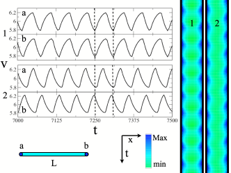
Figure 1: Oscillations of the membrane inhibitor $v$ in a one-dimensional bulk, bounded by two 0-dimensional “membranes”. The left panel shows time series in each of the two boundaries (denoted respectively by a and b). Two regimes are shown: in-phase and anti-phase oscillations, labeled “1” and “2”, and are obtained by setting $D_{V}=0.7$ and $D_{V}=0.3$, respectively. The two right panels show spatiotemporal representations of the inhibitor concentration in color code, with time running from top to bottom and space represented horizontally. The parameters used in these simulations are $L=10$, $\epsilon=0.015$, $k_{v}=5\epsilon$, $\sigma_{V}=D_{V}/100$ and $\sigma_{U}=D_{U}=k_{u}=0$. As initial condition, the system is set at the rest state with additional (small) spatial fluctuations, so that there is a slight heterogeneity in the initial concentration field.

For each regime, a plot of the time evolution of $v$ at the two boundaries is displayed. Additionally, spatiotemporal plots are shown in the right panels. The results clearly show not only that self-sustained oscillations appear even when the system is not intrinsically oscillatory, but that the oscillations can synchronize either in phase or in anti-phase. The behavior persists even when the system is perturbed by noise (data not shown), evidencing the robustness of the phenomenon. In Fig. 1, the inhibitor diffusion was varied in order to change the type of phase locking. As we show below, other parameters can be similarly tuned to control the system’s behavior.

Theoretical analysis in $d=1$. The effect of coupling on the behavior of the excitable membrane can be determined by using the solution and boundary conditions of the bulk equations (1)-(2) in the membrane equations (3)-(4). To that end, we determine the stationary solutions of the diffusion equations (1)-(2) in a one-dimensional region of length $L$. In the case of the inhibitor, the resulting density profile is $V(x)=V(0)\cosh\left[\sqrt{\frac{\sigma_{V}}{D_{V}}}(\frac{L}{2}-x)\right]/\cosh\left[\sqrt{\frac{\sigma_{V}}{D_{V}}}\frac{L}{2}\right]$, where $V(0)=v$. Its derivative at the boundary is then

$$V^{\prime}(x=0)=-v\sqrt{\frac{\sigma_{V}}{D_{V}}}\tanh\left[\sqrt{\frac{\sigma_{V}}{D_{V}}}\frac{L}{2}\right].$$ (7)

This expression, when inserted into the steady-state membrane equation

$$0=\epsilon g(u,v)+k_{v}V^{\prime}(x=0),$$ (8)

leads to a new effective inhibitor nulcline

$$v=\frac{z\;u}{1+\frac{l_{1}}{l_{0}}\tanh\left[\frac{L/2}{l_{0}}\right]}.$$ (9)

Here $l_{1}\equiv\frac{k_{v}}{\epsilon}$ and $l_{0}\equiv\sqrt{\frac{D_{V}}{\sigma_{V}}}$. Note that the initial inhibitor nulcline $v=zu$ is modified due to the coupling with the bulk, effectively decreasing its slope $z$ as the coupling increases. The same analysis can be done for the activator, although in that case, the contribution from the coupling with the bulk barely modifies the shape of the membrane $u$-nulcline [$f(u,v)=0)$], and therefore its effects will be ignored in what follows.

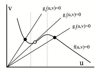
Figure 2: Qualitative scheme of the effect of the bulk on the nulclines of the excitable membrane. A full circle denotes a stable fixed point and an empty circle an unstable one. The $g$ nulcline labeled $g_{0}$ corresponds to the absence of coupling with the bulk. $g_{1}$ and $g_{2}$ define modified $v$-nulclines for increasing $k_{v}\neq 0$. The case of $g_{1}$ corresponds to a self-sustained oscillatory regime, while for larger coupling ($g_{2}$) the system is back at a steady state again. The $f$ nulcline is practically unmodified by the coupling, and is left unchanged in this schematic plot.

With the above considerations, we can now understand, both qualitatively and quantitatively, the effect of membrane-bulk coupling. As shown in Fig. 2, the effect of the diffusive and degrading bulk can be mapped to an effective variation of the slope of the $g(u,v)$ nulcline, yielding a change from an excitable situation where only one stable fixed point exists, to an oscillatory regime where the fixed point is unstable and a limit cycle (not shown) develops. Finally, large enough coupling even leads the system back again to an excitable regime. The result obtained in Eq. (9) shows that three length scales control the system’s behavior in the steady state: $L$, $l_{0}$ and $l_{1}$. The first one, $L$, is the natural length of the system. The second one, $l_{0}$, is a characteristic length determined by the ratio of the diffusion $D_{V}$ and the degradation $\sigma_{V}$, and corresponds to an action length of the bulk. Finally, the effect of the coupling enters directly through the combination of the coupling strength $k_{v}$ and the time scale ratio $\epsilon$, giving rise to a characteristic length scale $l_{1}$.

Making use of Eq. (9) and considering the location and the stability of the fixed point (determined by the crossing of the nulclines), we can analytically predict the region in parameter space where the system will behave as an oscillator. The corresponding phase diagram is shown in Fig. 3.

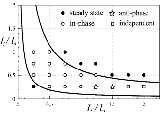
Figure 3: Phase diagram of a one-dimensional diffusive and degrading bulk delimited by two point excitable boundaries. Solid lines have been determined analytically. The oscillatory region lays within these lines. Symbols correspond to numerical simulations: full circles, stationary state; empty circles, in-phase oscillations; empty stars, anti-phase oscillations; empty squares, independent oscillations. Parameters are those of Fig. 1 except for $D_{V}=0.5$, and $k_{v}$ and $L$ are varied.

The theoretically predicted boundaries of the oscillatory region (solid lines in Fig. 3) agree very well with simulations. Therefore, the steady state analysis yields a clear understanding of why the excitable membrane becomes unstable and starts to oscillate. The second set of important properties of the system, i.e. synchronization and phase locking between the oscillating poles, have to be determined numerically. Such an investigation leads to different types of oscillatory regimes, as shown in Fig. 3, in which anti-phase oscillations (stars) separate the region of in-phase oscillations (empty circles) from a domain where the two poles of the system oscillate independently (squares), namely, having the same frequency but an undefined phase relation. Note that for large $L$ the pole oscillations can not interact, since the opposing membranes are too far away. On the other hand, for large enough $k_{v}$ (i.e. $l_{1}$) oscillations (when they occur) can only be in phase. Finally, we note that increasing the inhibitor diffusion coefficient $D_{V}$ makes $l_{0}$ shorter, which changes the overall scale of the phase diagram.

Extension to $d=2$: numerical simulations. Once the one-dimensional case is understood and fully characterized, we now consider a two-dimensional system with a rectangular geometry. The main difference is that now the membrane is also distributed in space (but without internal diffusion howard01 ), while in the previous case it was zero-dimensional. However, by analogy to the one-dimensional case the relevance of the different parameters can be understood, and again the same phenomena are encountered. Every parameter has an important physical meaning. $D_{V}$ is responsible for the indirect coupling between membrane elements and is thus a necessary ingredient for the synchronization. $D_{U}$ is crucial to avoid several pathologies that occur in $d>1$, such as accumulation of inhibitor along the membrane, which leads to local blocking of the oscillations. $\sigma_{V}$ is key to the spontaneous onset of local oscillations at the membrane, as we have already seen in the one-dimensional case. $k_{v}$ determines the new effective nulcline due to the influence of the bulk, and controls the synchronization phases.

Furthermore, there are now two length scales in the problem associated with the system size. $L_{1}$ is the length of the rectangular system and its width is denoted by $L_{2}$. Assuming $L_{1}>L_{2}$, we are interested in observing oscillations along $L_{1}$, mimicking the pole-to-pole oscillations in elongated bacteria. In this case, the lateral walls can dominate the main activity of the system, preventing anti-phase oscillations for short lengths. For very long lengths the communication is fragile. For intermediate lengths $L_{1}$, given that $L_{2}$ is smaller than $L_{1}$, we expect the oscillations along the minor axis to be more or less synchronized in phase, and not to disturb excessively the pole-to-pole oscillations.

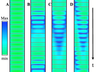
Figure 4: Temporal series of snapshots of $V$ in 2-dimensions. A. Steady state solution. B and C. In-phase periodic oscillations. D. Anti-phase periodic oscillations and traveling wave. The values of the parameters are $L_{1}=15.5$, $L_{1}/L_{2}=3.4$, $D_{U}=D_{V}=0.1$, $\sigma_{V}=0.00124$, $\sigma_{U}=10^{-4}\sigma_{V}$, $k_{u}=k_{v}\equiv k$ and $\epsilon=0.015$. The different regimes are obtained varying $k$: ${\bf A}$, $k=0.03$; ${\bf B}$, $k=0.08$; ${\bf C}$, $k=0.095$; and ${\bf D}$, $k=0.11$. Each snapshot is taken every $\Delta t=10$.

We now present the phenomenology that can be observed numerically in two dimensions. In Fig. 4, temporal sequences of two-dimensional snapshots of the density map of $V$ are displayed for different kinds of behavior. The system is initiated again from the rest state, superimposed with small random heterogeneous perturbations. When dynamical noise is added to the simulations, not only is synchronization maintained, but also the different regimes develop easier and faster. Figure 4A corresponds to small couplings, for which the system is unable to oscillate and remains in a stable fixed point, corresponding to the quiescent state of the excitable membranes. For larger coupling (panel B), in-phase oscillations emerge from the center of the system. Panel C shows a different kind of in-phase oscillation, which is governed by the poles of the system. Finally, panel D shows a traveling wave that leads to anti-phase oscillations of the poles, similarly to what was found in the one-dimensional case. The traveling wave alternates periodically and slowly its direction of motion, from left to right and vice versa (with a period larger than the time span shown in Fig. 4). In spite of these alternations, the poles oscillate periodically and in perfect anti-phase. The dimensionless parameters leading to this regime, given in the caption of Fig. 4, correspond to reasonable biological values when turned into dimensional units. For instance, just by assuming a bacterium of length $L\simeq 4\mu m$, it is found that $l_{0}\simeq 2.28\mu m$ and $l_{1}=1.88\mu m$.

Conclusions. We have reported a minimal mechanism that generates pole-to-pole oscillations in non-active elongated media. The mechanism relies on the interaction of the system’s bulk with an excitable (non-oscillatory) membrane, and can be understood analytically for one-dimensional bulks making use of a phase-plane picture of the membrane’s excitability. Both in-phase and anti-phase oscillations can be observed. In the case of a two-dimensional bulk, anti-phase dynamics is associated with a traveling wave that periodically reverses its propagation direction. This could be a generic mechanism leading to spatiotemporal oscillations in systems limited by active boundaries, such as cells.

This research was supported by Ministerio de Educacion y Ciencia (Spain) under project FIS2006-11452 and grant FPU-AP-2004-0770 (A.G-M), and by the Generalitat de Catalunya.

References

- (1) M.C. Cross and P.C. Hohenberg, Rev. Mod. Phys. 65, 851 (1993).
- (2) S. Y. Shvartsman, E. Schütz, R. Imbihl and I. G. Kevrekidis, Phys. Rev. Lett. 83, 2857 (1999).
- (3) N. Khrustova, G. Veser, A. Mikhailov, R. Imbihl, Phys. Rev. Lett. 75, 3564 (1995).
- (4) M. Yoneyama, A. Fujii, S. Maeda, Physica D 84 (1995) 120-125.
- (5) S. Ramaswamy, J. Toner, and J. Prost, Phys. Rev. Lett. 84, 3494 (2000).
- (6) H. Levine and W.-J. Rappel, Phys. Rev. E 72, 061912 (2005).
- (7) H. Meinhardt and P. A. J. de Boer, Proc. Natl. Acad. Sci. U.S.A. 98, 14202 (2001).
- (8) M. Howard and K. Kruse, J. Cell Biol. 168, 533 (2005).
- (9) M. Howard, A. D. Rutenberg, and S. de Vet, Phys. Rev. Lett. 87, 278102 (2001).
- (10) K. Kruse, Biophys. J. 82, 618 (2002).
- (11) K. C. Huang, Y. Meir, and N. S. Wingreen, Proc. Natl. Acad. Sci. U.S.A. 100, 12724 (2003).
- (12) R. V. Kulkarni, K. C. Huang, M. Kloster, and N. S. Wingreen, Phys. Rev. Lett. 93, 228103 (2004).
- (13) D. A. Drew, M. J. Osborn, and L. I. Rothfield, Proc. Natl. Acad. Sci. U.S.A. 102, 6114 (2005).
- (14) A.S. Mikhailov, Foundations of synergetics I: Distributed active systems, 2nd Ed. (Springer, Berlin, 1994).
- (15) B. Pando, J. E. Pearson, and S. P. Dawson, Phys. Rev. Lett. 91, 258101 (2003).
- (16) Particularizing to the Min system in E. coli, the activator would correspond to the protein MinD, and the inhibitor to the protein MinE. In fact, MinD is known to self-associate in the cell wall, where it recruits MinE, which in turn releases MinD back to the cytoplasm meinhardt .