Confined coherence in quasi-one-dimensional metals

Abstract

We present a functional renormalization group calculation of the effect of strong interactions on the shape of the Fermi surface of weakly coupled metallic chains. In the regime where the bare interchain hopping is small, we show that scattering processes involving large momentum transfers perpendicular to the chains can completely destroy the warping of the true Fermi surface, leading to a confined state where the renormalized interchain hopping vanishes and a coherent motion perpendicular to the chains is impossible.

Introduction. Electron-electron interactions can strongly modify the Fermi surface (FS) of a metal. A well known example is the Pomeranchuk transition, where the symmetry of the FS is spontaneously broken due to strong interactions in the zero-sound channel Pomeranchuk58 . However, there are other quantum phase transitions associated with the geometry or the topology of the FS without symmetry breaking, such as the Lifshitz transition Lifshitz60 ; Quintanilla06 or the truncation transition Furukawa98 ; Ferraz03 , where certain sectors of the FS are washed out by interactions, while others remain intact. Another example is the interaction-induced confinement transition, which has been proposed by Clarke, Strong, and Anderson more than ten years ago Clarke94 : they considered metallic chains with small interchain hopping $t_{\bot,0}$. For weak interactions, the FS consists then of two disconnected weakly curved sheets as shown Fig. 1.

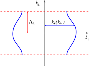
Figure 1: (Color online) FS of a two-dimensional array of weakly coupled metallic chains. The dashed lines mark the boundary of the first Brillouin zone in the direction perpendicular to the chains.

The amplitude of the warping of the FS is proportional to the renormalized interchain hopping $t_{\bot}$. Clarke et al. Clarke94 suggested that, at least for sufficiently strong interactions and small $t_{\bot,0}$, the renormalized $t_{\bot}$ vanishes. The true FS is then completely flat, so that a coherent motion of the electrons in the direction perpendicular to the chains is not possible (confined coherence).

In the past decade the confinement problem in weakly coupled metallic chains has been studied by many authors Clarke94 ; Wen90 ; Kopietz94 ; Boies95 ; Arrigoni98 , but the results have not converged due to a lack of controlled methods. A simple one-loop calculation Wen90 ; Boies95 suggests that the renormalized interchain hopping vanishes if the anomalous dimension $\eta$ of the Luttinger liquid state without interchain hopping is larger than unity. However, this argument does not take the renormalization of $\eta$ by interchain hopping into account. Indeed, more refined calculations by Arrigoni Arrigoni98 suggest that higher order corrections are important and possibly lead to a finite $t_{\bot}$ even for $\eta>1$. In this Letter we shall re-examine this problem using a novel functional renormalization group (RG) approach involving both fermionic and bosonic fields Schuetz05 ; Ledowski07 . Our main result is that the regime of confined coherence proposed in Ref. Clarke94 indeed exists, so that strong interactions can give rise to a non-Fermi liquid normal state in quasi-one-dimensional metals.

Model. We start from an effective low energy model for spinless fermions with linearized energy dispersion and density-density interactions. The Euclidean action is

$$S[\bar{\psi},\psi] = \sum_{\alpha}\int_{K}\bigl{[}-i\omega+\alpha v_{F}\delta k_{\parallel}+\mu_{0}(k_{\bot})\bigr{]}\bar{\psi}_{K\alpha}{\psi}_{K\alpha}$$ (1)

$$+ \frac{1}{2}\sum_{\alpha\alpha^{\prime}}\int_{\bar{K}}f_{\alpha\alpha^{\prime}}\bar{\rho}_{\bar{K}\alpha}\rho_{\bar{K}\alpha^{\prime}}\;,$$

where $\mu_{0}(k_{\bot})=-\Sigma({\bm{k}}_{F},i0)$ is a counter-term involving the exact self-energy at the true FS ${\bm{k}}={\bm{k}}_{F}$ and zero frequency, and $\delta k_{\parallel}=k_{\parallel}-\alpha k_{F}(k_{\bot})$. Here $k_{\parallel}$ is the component of the two-dimensional lattice momentum $\bm{k}$ parallel to the chain direction, and $k_{\bot}$ is the corresponding perpendicular component. The FS $\bm{k}_{F}$ can then be parameterized as $k_{\parallel}=\alpha k_{F}(k_{\bot})$, where $\alpha=\pm 1$ labels the two disconnected sheets of the FS, see Fig. 1. We neglect the $k_{\bot}$-dependence of the Fermi velocity $v_{F}$. The chiral fields $\psi_{K\alpha}$ are defined in terms of the usual Fermi fields $\psi_{k_{\parallel},k_{\bot},i\omega}$ via $\psi_{K\alpha}=\psi_{\alpha k_{F}(k_{\bot})+\delta k_{\parallel},k_{\bot},i\omega}$, and the chiral densities $\rho_{\bar{K}\alpha}$ are $\rho_{\bar{K}\alpha}=\int_{K}\bar{\psi}_{K\alpha}\psi_{K+\bar{K}\alpha}$. We use collective labels $K=(\delta k_{\parallel},k_{\bot},i\omega)$ for fermionic and $\bar{K}=(\bar{k}_{\parallel},\bar{k}_{\bot},i\bar{\omega})$ for bosonic fields, where $\omega$ and $\bar{\omega}$ are Matsubara frequencies. The integration symbols are $\int_{K}=\int_{k_{\bot}}\int_{-\Lambda_{\parallel}}^{\Lambda_{\parallel}}\frac{d\delta k_{\parallel}}{2\pi}\int\frac{d\omega}{2\pi}$ and $\int_{\bar{K}}=\int_{\bar{k}_{\bot}}\int_{-\bar{\Lambda}_{\parallel}}^{\bar{\Lambda}_{\parallel}}\frac{d\bar{k}_{\parallel}}{2\pi}\int\frac{d\bar{\omega}}{2\pi}$ where for later convenience we have introduced the notation $\int_{k_{\bot}}=\int_{-\Lambda_{\bot}}^{\Lambda_{\bot}}\frac{dk_{\bot}}{2\Lambda_{\bot}}$ and $\int_{\bar{k}_{\bot}}=\int_{-\bar{\Lambda}_{\bot}}^{\bar{\Lambda}_{\bot}}\frac{d\bar{k}_{\bot}}{2\bar{\Lambda}_{\bot}}$. Here $\Lambda_{\parallel}$ is a bandwidth cutoff, $\Lambda_{\bot}=\pi/a_{\bot}$ is the width of the Brillouin zone in transverse direction, and $\bar{\Lambda}_{\bot}$ and $\bar{\Lambda}_{\parallel}$ restrict the momentum transfered by the interaction in the directions parallel and perpendicular to the chains. We assume that $\bar{\Lambda}_{\parallel}\ll{\rm min}\{k_{F}(k_{\bot})\}$, so that the interaction $f_{\alpha\alpha^{\prime}}$ in Eq. (1) does not transfer momentum between the two disconnected sheets of the FS. However, the transverse momentum transfer cutoff $\bar{\Lambda}_{\bot}$ can be of the order of the transverse width $\Lambda_{\bot}=\pi/a_{\bot}$ of the Brillouin zone, so that transverse Umklapp scattering is possible. For simplicity we set $\bar{\Lambda}_{\bot}=\Lambda_{\bot}$ and call $\bar{\Lambda}_{\parallel}=\Lambda_{0}$.

Self-consistent perturbation theory. To begin with, let us calculate the FS within second order self-consistent perturbation theory. Using the procedure outlined in Ref. [Neumayr03, ], we obtain the following integral equation for the difference $\delta{k}_{F}(k_{\bot})=k_{F}(k_{\bot})-k_{F,0}(k_{\bot})$ between the true Fermi momentum $k_{F}(k_{\bot})$ and the corresponding $k_{F,0}(k_{\bot})$ without interactions at the same density,

$$\frac{\delta{k}_{F}(k_{\bot})}{\Lambda_{0}} = \left[-{g}_{4}+\frac{{g}_{4}^{2}+{g}_{2}^{2}}{2}\right]\int_{\bar{k}_{\bot}}\tilde{\Delta}(k_{\bot},\bar{k}_{\bot})$$ (2)

$$-{g}_{2}^{2}\int_{\bar{k}_{\bot}}\int_{k_{\bot}^{\prime}}J(\tilde{\Delta}(k_{\bot},\bar{k}_{\bot});\tilde{\Delta}(k_{\bot}^{\prime},\bar{k}_{\bot}))\;,$$

where $\tilde{\Delta}(k_{\bot},\bar{k}_{\bot})=[k_{F}(k_{\bot})-k_{F}(k_{\bot}+\bar{k}_{\bot})]/{\Lambda}_{0}$, and

$$J(\tilde{\Delta};\tilde{\Delta}^{\prime})=\frac{\tilde{\Delta}+\tilde{\Delta}^{\prime}}{4}\ln\left[\frac{4-(\tilde{\Delta}-\tilde{\Delta}^{\prime})^{2}}{(\tilde{\Delta}+\tilde{\Delta}^{\prime})^{2}}\right]\;.$$ (3)

The dimensionless couplings $g_{2}$ and $g_{4}$ are defined via $2\pi g_{4}=\nu_{0}f_{++}=\nu_{0}f_{--}$ and $2\pi g_{2}=\nu_{0}f_{+-}=\nu_{0}f_{-+}$, where the factor $\nu_{0}=\Lambda_{\bot}(\pi v_{F})^{-1}=(a_{\bot}v_{F})^{-1}$ is introduced for convenience. We have solved Eq. (2) numerically, but for small $t_{\bot}$ we can also obtain an approximate analytic solution using the fact that in this case the dominant renormalization of the FS is due to the logarithmic term in Eq. (3). Suppose that the bare FS is of the form $k_{F,0}(k_{\bot})=\bar{k}_{F}+t_{0}\cos(k_{\bot}a_{\bot})$ where $t_{0}=2t_{\bot,0}/v_{F}\ll\Lambda_{0}$ and the average $\bar{k}_{F}$ is fixed by the total density. The renormalized FS is then given by $k_{F}(k_{\bot})=\bar{k}_{F}+t\cos(k_{\bot}a_{\bot})+\ldots$, where $t$ is proportional to the renormalized nearest neighbor interchain hopping, and the ellipsis denotes higher harmonics corresponding to longer range hoppings. From the numerical solution of the integral equation (2) we find that for $g_{2},g_{4}\ll 1$ the higher harmonics are indeed small. Then Eq. (2) can be reduced to a transcendental equation for $t$, which to leading logarithmic order in $t/\Lambda_{0}$ can be written as $t/t_{0}=[1+R(t)]^{-1}$, with

$$R(t)\approx\frac{g_{4}}{2}-\frac{{g}_{4}^{2}}{4}+\frac{{g}_{2}^{2}}{2}\ln({\Lambda}_{0}/|t|)\;.$$ (4)

A similar relation has been obtained previously Fabrizio93 ; Ledowski07 for the difference between the Fermi momenta associated with the bonding and the anti-bonding band in two coupled spinless chains. Note that to first order in the bare interaction $R(t)\propto{g}_{4}$, so that a repulsive interaction ${g}_{4}>0$ reduces the warping of the FS, while for ${g}_{4}<0$ the warping of the FS is enhanced. However, for $t_{\bot}\rightarrow 0$ the logarithmic term proportional to ${g}_{2}^{2}$ always dominates and predicts an interaction-induced reduction of the FS warping, irrespective of the sign of the interaction.

Functional RG approach. We now generalize the RG approach developed in Ref. [Ledowski07, ] in the context of a simplified two-chain model to the more interesting two-dimensional case considered here. The method has been described in detail previously Ledowski07 , so that we will be rather brief here. In the momentum transfer cutoff scheme Schuetz05 we decouple the density-density interaction by means of a bosonic Hubbard-Stratonovich transformation and then use the maximal momentum carried by the boson field as flow parameter $\Lambda$ of the RG. Our initial cutoff is thus $\Lambda=\Lambda_{0}=\bar{\Lambda}_{\parallel}$. Eliminating boson fields with momenta in the range $\Lambda<|\bar{k}_{\parallel}|<\Lambda_{0}$ we obtain a new effective action, whose vertices are determined by a formally exact hierarchy of functional RG flow equations. To calculate the true FS, we need the flow equation for the relevant part $r_{l}(k_{\bot})$ of the irreducible fermionic self-energy $\Sigma_{\Lambda}(K,\alpha)$, which is defined via $r_{l}(k_{\bot})=Z_{l}(k_{\bot})[\Sigma_{\Lambda}({\bm{k}}_{F},i0,\alpha)+\mu_{0}(k_{\bot})]/v_{F}\Lambda$. Here $l=\ln(\Lambda_{0}/\Lambda)$ and $Z_{l}(k_{\bot})$ is the flowing wave-function renormalization. The functional RG flow equation for $r_{l}(k_{\bot})$ is of the form

$$\partial_{l}r_{l}(k_{\bot})=[1-\eta_{l}(k_{\bot})]r_{l}(k_{\bot})+\dot{\Gamma}_{l}(k_{\bot})\;,$$ (5)

where $\eta_{l}(k_{\bot})=-\partial_{l}\ln Z_{l}(k_{\bot})$ is the flowing anomalous dimension. An approximate expression for the inhomogeneity $\dot{\Gamma}_{l}(k_{\bot})$ is given in Eq. (7) below. As long as $\eta_{\infty}(k_{\bot})<1$, the FS is well defined. The shift $\delta k_{F}(k_{\bot})$ of the FS due to interactions can then be obtained from the requirement that the initial value $r_{0}(k_{\bot})$ should be fine tuned so that the relevant coupling $r_{l}(k_{\bot})$ flows into a fixed point Kopietz01 . This leads to the following exact integral equation for the FS,

$$\frac{\delta k_{F}(k_{\bot})}{\Lambda_{0}}=r_{0}(k_{\bot})=-\int_{0}^{\infty}dle^{-l+\int_{0}^{l}dt\eta_{t}(k_{\bot})}\dot{\Gamma}_{l}(k_{\bot})\;.$$ (6)

Using the same truncation strategy as in Ref. [Ledowski07, ], we approximate

$$\dot{\Gamma}_{l}(k_{\bot}) = -\int_{\bar{k}_{\bot}}\int\frac{d\bar{q}d\bar{\epsilon}}{(2\pi)^{2}}\frac{\delta(|\bar{q}|-1)[{\bf{F}}_{l}(\bar{q},i\bar{\epsilon},\bar{k}_{\bot})]_{\alpha\alpha}e^{i\bar{\epsilon}0}}{i\bar{\epsilon}-\alpha\bar{q}-\tilde{\Delta}_{l}(k_{\bot},\bar{k}_{\bot})}$$ (7)

$$\times\gamma_{l}(k_{\bot},\bar{k}_{\bot})\gamma_{l}(k_{\bot}+\bar{k}_{\bot},-\bar{k}_{\bot})\;,$$

where $\tilde{\Delta}_{l}(k_{\bot},\bar{k}_{\bot})=\tilde{k}_{F,l}(k_{\bot})-\tilde{k}_{F,l}(k_{\bot}+\bar{k}_{\bot})$ with $\tilde{k}_{F,l}(k_{\bot})=k_{F}(k_{\bot})/\Lambda-r_{l}(k_{\bot})$. The inverse of the $2\times 2$-matrix ${\bf{F}}_{l}(\bar{q},i\bar{\epsilon},\bar{k}_{\bot})$ is defined via

$$[{\bf{F}}_{l}(\bar{q},i\bar{\epsilon},\bar{k}_{\bot})]^{-1}_{\alpha\alpha^{\prime}}=[\nu_{0}{\bf{f}}]^{-1}_{\alpha\alpha^{\prime}}+\delta_{\alpha\alpha^{\prime}}\tilde{\Pi}_{l}(\bar{q},i\bar{\epsilon},\bar{k}_{\bot},\alpha)\;,$$ (8)

where $\bf{f}$ is a matrix in chirality space with elements $[{\bf{f}}]_{\alpha\alpha^{\prime}}=f_{\alpha\alpha^{\prime}}$, and $\tilde{\Pi}_{l}(\bar{q},i\bar{\epsilon},\bar{k}_{\bot},\alpha)$ is the rescaled polarization associated with fermions of chirality $\alpha$, for which we use the adiabatic approximation Ledowski07

$$\tilde{\Pi}_{l}(\bar{q},i\bar{\epsilon},\bar{k}_{\bot},\alpha) = \frac{1}{2\pi}\int_{k_{\bot}}\frac{\tilde{\Delta}_{l}(k_{\bot},\bar{k}_{\bot})+\alpha\bar{q}}{\tilde{\Delta}_{l}(k_{\bot},\bar{k}_{\bot})+\alpha\bar{q}-i\bar{\epsilon}}$$

$$\times \gamma_{l}(k_{\bot},\bar{k}_{\bot})\gamma_{l}(k_{\bot}+\bar{k}_{\bot},-\bar{k}_{\bot})\;.$$ (9)

The anomalous dimension is in this approximation

$$\eta_{l}(k_{\bot}) = -\int_{\bar{k}_{\bot}}\int\frac{d\bar{q}d\bar{\epsilon}}{(2\pi)^{2}}\frac{\delta(|\bar{q}|-1)[{\bf{F}}_{l}(\bar{q},i\bar{\epsilon},\bar{k}_{\bot})]_{\alpha\alpha}}{[i\bar{\epsilon}-\alpha\bar{q}-\tilde{\Delta}_{l}(k_{\bot},\bar{k}_{\bot})]^{2}}$$ (10)

$$\times\gamma_{l}(k_{\bot},\bar{k}_{\bot})\gamma_{l}(k_{\bot}+\bar{k}_{\bot},-\bar{k}_{\bot})\;.$$

Finally, the dimensionless vertex $\gamma_{l}(k_{\bot},\bar{k}_{\bot})$ with one bosonic and two fermionic external legs (where $k_{\bot}$ labels the incoming fermion and $\bar{k}_{\bot}$ labels the boson) satisfies the flow equation

$$\partial_{l}\gamma_{l}(k_{\bot},\bar{k}_{\bot}) = -\frac{1}{2}[\eta_{l}(k_{\bot})+\eta_{l}(k_{\bot}+\bar{k}_{\bot})]\gamma_{l}(k_{\bot},\bar{k}_{\bot})$$

$$-\int_{\bar{k}_{\bot}^{\prime}}\int\frac{d\bar{q}d\bar{\epsilon}}{(2\pi)^{2}}\delta(|\bar{q}|-1)[{\bf{F}}_{l}(\bar{q},i\bar{\epsilon},\bar{k}_{\bot}^{\prime})]_{\alpha\alpha}$$

$$\times\frac{\gamma_{l}(k_{\bot}+\bar{k}_{\bot}^{\prime},\bar{k}_{\bot})\gamma_{l}(k_{\bot},\bar{k}_{\bot}^{\prime})\gamma_{l}(k_{\bot}+\bar{k}_{\bot}+\bar{k}_{\bot}^{\prime},-\bar{k}_{\bot}^{\prime})}{[i\bar{\epsilon}-\alpha\bar{q}-\tilde{\Delta}_{l}(k_{\bot},\bar{k}_{\bot}^{\prime})][i\bar{\epsilon}-\alpha\bar{q}-\tilde{\Delta}_{l}(k_{\bot}+\bar{k}_{\bot},\bar{k}_{\bot}^{\prime})]}\;,$$

with initial condition $\gamma_{l=0}(k_{\bot},\bar{k}_{\bot})=1$. A graphical representation of Eq. (LABEL:eq:gammaflow) is shown in Fig. 2.

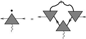
Figure 2: Diagrammatic representation of the flow equation (LABEL:eq:gammaflow) for the three-legged vertex with one bosonic (wavy line) and two fermionic (solid lines with arrows) external legs. The thick wavy line with a slash denotes the bosonic single scale propagator. Additional contributions involving irrelevant higher order vertices are omitted, see Refs. [Schuetz05, ; Ledowski07, ].

Results. Eqs. (5)-(LABEL:eq:gammaflow) form a closed system of flow equations for the rescaled self-energy at the FS $r_{l}(k_{\bot})$, the flowing anomalous dimension $\eta_{l}(k_{\bot})$, and the three-legged vertex $\gamma_{l}(k_{\bot},\bar{k}_{\bot})$. Of course, these equations can only be solved numerically, but the qualitative behavior of the solutions can also be extracted analytically. To begin with, let us establish the relation with the perturbative Eq. (2). We set $g_{4}=0$ from now on, because the dominant renormalization of the FS is due to the $g_{2}$-process. In the simplest approximation, we set $\gamma_{l}(k_{\bot},\bar{k}_{\bot})\approx 1$, $\eta_{l}(k_{\bot})\approx 0$ and replace the flowing FS $\tilde{k}_{F,l}(k_{\bot})=k_{F}(k_{\bot})/\Lambda-r_{l}(k_{\bot})$ by $k_{F}(k_{\bot})/\Lambda$. Then we obtain from Eqs. (6) and (7) to leading logarithmic order

$$\frac{\delta k_{F}(k_{\bot})}{\Lambda_{0}}=[(1-g_{2}^{2})^{-\frac{1}{2}}-1]\int_{\bar{k}_{\bot}}\tilde{\Delta}(k_{\bot},\bar{k}_{\bot})\ln|\tilde{\Delta}(k_{\bot},\bar{k}_{\bot})|\;.$$ (12)

Expanding in harmonics we obtain as before $t/t_{0}=[1+R(t)]^{-1}$, but now with

$$R(t) \approx [(1-g_{2}^{2})^{-\frac{1}{2}}-1]\ln({\Lambda_{0}}/{|t|})\;,$$ (13)

which reduces to Eq. (4) to leading order in $g_{2}$. Obviously, $R(t)\rightarrow\infty$ for $g_{2}\rightarrow 1$, indicating a confinement transition at strong coupling, where the renormalized interchain hopping $t$ vanishes. However, from our previous work on two coupled chains Ledowski07 we know that vertex corrections and wave-function renormalizations can possibly change this scenario.

To investigate this, let us first consider the RG flow of the vertex $\gamma_{l}(k_{\bot},\bar{k}_{\bot})$ numerically. Representative results are shown in Fig. 3.

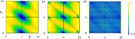
Figure 3: (Color online) Typical evolution of the vertex $\gamma_{l}(k_{\bot},\bar{k}_{\bot})$ for different values of the flow parameter $l$. To evaluate the flow we have expanded in Eqs. (7) and (LABEL:eq:gammaflow) up to $g_{2}^{2}$. We have assumed a harmonic bare FS with amplitude $t_{0}/\Lambda_{0}=10^{-3}$ and bare coupling $g_{2}=0.4$ From left to right $l=\frac{1}{2}l_{c},l_{c},3l_{c}$ and $\gamma_{\min}=0.999989,0.981,0.85$, where the crossover scale $l_{c}$ (see text) can be approximated by $l_{c}\approx-\ln(2t_{0}/\Lambda_{0})$ for small $g_{2}$.

Obviously, the dependence of $\gamma_{l}(k_{\bot},\bar{k}_{\bot})$ on the fermionic momentum $k_{\bot}$, which develops at intermediate scales $l$, is smoothed out again at the scale $l_{c}$ where the reduced cutoff $\Lambda_{c}=\Lambda_{0}e^{-l_{c}}$ becomes comparable with the warping of the renormalized FS. Defining the flowing dimensionless nearest neighbor interchain hopping $\tilde{t}_{l}$ via $\tilde{k}_{F,l}=\bar{k}_{F}/\Lambda+\tilde{t}_{l}\cos(k_{\bot}a_{\bot})+\ldots$, the crossover scale $l_{c}$ can be defined self-consistently via $2\tilde{t}_{l=l_{c}}=1$. Because of the weak dependence of $\gamma_{l}(k_{\bot},\bar{k}_{\bot})$ on the fermionic momentum ${k}_{\bot}$, we may approximate $\gamma_{l}(k_{\bot},\bar{k}_{\bot})\approx\gamma_{l}(0,\bar{k}_{\bot})\equiv\gamma_{l}(\bar{k}_{\bot})$. Moreover, using the fact that close to the confinement transition $|\tilde{t}_{l}|\ll 1$, we obtain from Eqs. (5)-(LABEL:eq:gammaflow) to leading order in $\tilde{t}_{l}$ the following RG flow equation for the effective interaction $g_{l}(\bar{k}_{\bot})=g_{2}\gamma_{l}^{2}(\bar{k}_{\bot})$,

$$\partial_{l}g_{l}(\bar{k}_{\bot})=-\frac{4\sin^{2}(\bar{k}_{\bot}a_{\bot}/2)g_{l}(\bar{k}_{\bot})u_{l}^{2}\tilde{t}_{l}^{2}}{\sqrt{1-u_{l}^{2}}[1+\sqrt{1-u_{l}^{2}}]^{3}}\;,$$ (14)

with $u_{l}=g_{l}(\pi/a_{\bot})$. Note that the flow of $g_{l}(\bar{k}_{\bot})$ is driven by the component $g_{l}(\pi/a_{\bot})$ of the interaction involving momentum transfer $\bar{k}_{\bot}=\pi/a_{\bot}$; in a simplified two-chain model this corresponds to the pair-tunneling process Fabrizio93 . The flow of the rescaled interchain hopping $\tilde{t}_{l}$ is determined by $\partial_{l}\tilde{t}_{l}=(1-\bar{\eta}_{l})\tilde{t}_{l}+O(\tilde{t}_{l}^{2})$, where $\bar{\eta}_{l}$ is the weighted FS average $\bar{\eta}_{l}=2\int_{{k}_{\bot}}\sin^{2}({k}_{\bot}a_{\bot}/2)\eta_{l}({k}_{\bot})$ of the flowing anomalous dimension, which for small $\tilde{t}_{l}$ can be approximated by $\eta_{l}(k_{\bot})=[1-g_{l}^{2}(k_{\bot})]^{-\frac{1}{2}}-1$. From the numerical solution of these equations we find that, for a given $t_{\bot,0}\ll v_{F}\Lambda_{0}$, there exists a critical value of the bare interaction $g_{2}$ where the renormalized $\tilde{t}=\tilde{t}_{\infty}$ vanishes, corresponding to a confinement transition to a state with vanishing interchain hopping $t_{\bot}$ and flat FS. 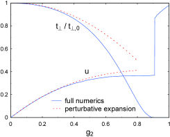In Fig. 4 we show the ratio $t_{\bot}/t_{\bot,0}$ together with the renormalized interaction $u=g_{\infty}(\pi/a_{\bot})$ as a function of the bare interaction for small $\tilde{t}_{0}=2t_{\bot,0}/(v_{F}\Lambda_{0})$.

Figure 4: (Color online) Renormalized nearest neighbor interchain hopping $t_{\bot}$ and renormalized interaction $u=g_{\infty}(\pi/a_{\bot})$ as a function of the bare interaction $g_{2}$ for $\tilde{t}_{0}=2t_{\bot,0}/(v_{F}\Lambda_{0})=0.1$ as obtained from the numerical solution of Eqs. (7) and (LABEL:eq:gammaflow). For the perturbative curves we have expanded in these equations up to order $g_{2}^{2}$.

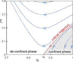
A projection of the RG flow in the $\tilde{t}$-$u$ plane is shown in Fig. 5.

Figure 5: (Color online) Projection of the RG flow in the $\tilde{t}$-$u$ plane. The trajectories are obtained from the numerical solution of Eq.(14) and $\tilde{t}_{l}=(1-\bar{\eta}_{l})\tilde{t}_{l}$, where $\bar{\eta}_{l}$ is the weighted FS average of the flowing anomalous dimension $\eta_{l}(k_{\bot})$ defined in the text.

At the confinement transition the system is certainly not a Fermi liquid, because the anomalous dimension $\eta_{l}(k_{\bot})$ is larger than unity and a sharp FS cannot be defined Kopietz01 . The physical properties of the model in the confined phase remain to be explored.

Summary and conclusions. We have shown that sufficiently strong interactions involving momentum transfers parallel to the chains can lead to a confinement transition in highly anisotropic quasi-one-dimensional metals. At the confinement transition the curvature of the two disconnected sheets of the FS vanishes, so that a coherent motion of the electrons perpendicular to the chains is not possible and the electronic motion is one-dimensional. Our calculation thus supports the existence of a confined state in quasi-one-dimensional metals, as originally suggested by Clarke, Strong, and Anderson Clarke94 . In the confined state the system is a non-Fermi liquid with large anomalous dimension. From the numerical solution of our functional RG equations we found no evidence for a truncation transition Furukawa98 ; Ferraz03 , where only certain sectors of the FS are washed out by interactions.

Because in this work we have considered only spinless fermions and interactions which do not transfer momentum between the two disconnected sheets of the FS, our model (1) is too simple to describe the competition between confinement and the tendency to develop some kind of long-range order, such as charge-density or spin-density waves. In principle, spin fluctuations can be taken into account with the help of another Hubbard-Stratonovich field, but the analysis of the resulting RG equations for the coupled boson-fermion model requires a substantial extension of our calculation.

We thank A. Ferraz and F. H. L. Essler for useful discussions.

References

(1)
I. J. Pomeranchuk, Zh. Eksp. Teor. Fiz. 35, 524 (1958)
[Sov. Phys. JETP 8, 361 (1958)].
(2)
I. M. Lifshitz, Zh. Eksp. Teor. Fiz. 38, 1569 (1960)
[Sov. Phys. JETP 11, 1130 (1960)].
(3)
J. Quintanilla and A. J. Schofield, Phys. Rev. B 74, 115126 (2006).
(4)
N. Furukawa, T. M. Rice, and M. Salmhofer, Phys. Rev. Lett.
81, 3195 (1998);
C. Honerkamp, M. Salmhofer, N. Furukawa, and T. M. Rice,
Phys. Rev. B 63, 035109 (2001).
(5)
A. Ferraz, Phys. Rev. B 68, 075115 (2003); H. Freire, E. Correa, and
A. Ferraz, ibid.71, 165113 (2005).
(6)
D. G. Clarke, S. P. Strong, and P. W. Anderson,
Phys. Rev. Lett. 72, 3218 (1994);
ibid.74, 4499 (1995); D. G. Clarke and S. P.
Strong, Adv. Phys. 46, 454 (1997).
(7)
X. G. Wen, Phys. Rev. B 42, 6623 (1990).
(8)
P. Kopietz, V. Meden, and K. Schönhammer, Phys. Rev. Lett.
74, 2997 (1995); Phys. Rev. B 56, 7232 (1997).
(9)
D. Boies, C. Bourbonnais and A.-M. S. Tremblay, Phys. Rev. Lett. 74, 968 (1995).
(10)
E. Arrigoni, Phys. Rev. Lett. 80, 790 (1998);
ibid.83, 128 (1999);
Phys. Rev. B 61, 7909 (2000).
(11)
F. Schütz, L. Bartosch, and P. Kopietz,
Phys. Rev. B 72, 035107 (2005).
(12)
S. Ledowski and P. Kopietz, Phys. Rev. B 75, 045134 (2007).
(13)
A. Neumayr and W. Metzner, Phys. Rev. B 67, 035112 (2003).
(14)
M. Fabrizio, Phys. Rev. B 48, 15838 (1993);
S. Ledowski, P. Kopietz, and A. Ferraz, ibid.71, 235106 (2005).
(15)
P. Kopietz and T. Busche, Phys. Rev. B 64, 155101 (2001);
S. Ledowski and P. Kopietz, J. Phys.: Condens. Matter 15, 4779 (2003).