Nonequilibrium tricriticality in one dimension

Abstract

We show the existence of a nonequilibrium tricritical point induced by a repulsive interaction in one dimensional asymmetric exclusion processes. The tricritical point is associated with the particle-hole symmetry breaking introduced by the repulsion. The phase diagram and the crossover in the neighbourhood of the tricritical point for the shock formation at one of the boundaries are determined.

The lack of any free energy like entity to describe nonequilibrium steady states makes general studies of nonequilibrium phase transitions rather difficult. For this reason, eventhough different types of phase diagrams are known with first-order or continuous phase transitions, and critical points from various case studiesderrida1 ; frey ; evans ; smsmb ; smvm , generalizations of these results are not straightforward. Since steady states are the closest analogs of equilibrium states (both being stationary in time), it is important to know how far the richness of the equilibrium critical phenomena with their connections to symmetrieshuang can be found in nonequilibrium systems.

This paper shows the bifurcation of a line of critical points through a tricritical pointhuang ; ahar in the phase diagram of a one dimensional interacting driven system as one interaction parameter is tuned. A tricritical point is also a point where a first order transition changes over to a continuous one, the pair of critical lines being the edges of two first order surfaces. We do observe such equilibrium-like gross features in the nonequilibrium system so as to classify it as a tricritical point, but, unlike equilibrium systems, all happening in one dimension.

The occurrence of a tricritical point in any system is significant because it implies a confluence of two different phenomena. As a consequence, the tricritical point controls the scaling description in its neighbourhood. Known examples from equilibrium systems include the $\theta$-point of polymer solutionsdegen , bunching and phase separation of steps on crystal surfacessmbsi , different transitions in magnetsahar , current hunt for a tricritical point in quark-gluon plasma in the context of early universeqgp , and many otherscomm . In equilibrium systems, a tricritical point is one in the hierarchy of critical points and corresponds to the case of three relevant variables as opposed to two for an ordinary critical point, as e.g., temperature and magnetic field for a Curie point of a magnet. In the Landau theory of phase transitions, the sequence of critical, tricritical points … occur as new symmetric minima in the Landau function develop. In analogy with that, we find in the nonequilibrium problem in hand, the tricriticality is associated with a particle-hole symmetry breaking or successive occurrences of peaks in the current in the system, that allows maximum current through the system at two different densities.

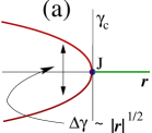
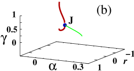
Figure 1: (a) The critical lines in the $\gamma$-$r$ plane, where $r=\varepsilon-\varepsilon_{J}$. The width vanishes with a characteristic exponent as $r\to 0-$. (b) Three dimensional view of the tricritical point J in the $\alpha$-$\gamma$-$r$ space. Only the critical lines are shown. These lines are nonplanar and (a) shows the projection.

Our results are based on a class of well-studied one-dimensional models for interacting particles moving on a track, which are variants of the asymmetric exclusion process (ASEP). There is current interest in these models because of the recent observation of localized shock phases and associated criticality. A shock in these models is a discontinuity in the steady state density along the track. Let us consider a one-dimensional lattice with particles injected at site $i=0$ at a rate $\alpha$ and withdrawn at $i=N$ at a rate $1-\gamma$. The particles hop to the right with mutual exclusion so that the occupation number at a site is $0$ or $1$. In addition, there is a next nearest neighbour repulsionhager so that a configuration

$$1100 \to 1010\qquad{\rm with\ a\ rate\ }1+\varepsilon,$$

$$0101 \to 0011\qquad{\rm at\ a\ rate\ }1-\varepsilon,$$

with ($0<\varepsilon<1$), where occupied and unoccupied states of a site are represented by $1$ and $0$ respectively. The hopping process is particle conserving. With a nonvanishing current, the system can evolve to a nonequilibrium steady state. Nonconservation is introduced by allowing evaporation or desorption ($1\to 0$) at a rate $\omega_{d}$ and deposition or adsorption ($0\to 1$) at a rate $\omega_{a}$ of particles at any site on the track. This dynamics, called the Langmuir dynamics, can maintain a density

$$\rho_{L}=\frac{\omega_{a}}{\omega_{a}+\omega_{d}}\neq\frac{1}{2}\quad{\rm if}\ \omega_{a}\neq\omega_{d}.$$ (1)

This is an equilibrium-like process with no current in the system. If the net flux due to adsorption/desorption is comparable to the hopping current, there will be a competition between the attempt to equilibrate and the drive to the nonequilibrium steady state. As a result, one gets new features like a shock phase, critical points one would not get otherwise.

For large $N$, we may use a continuum notation $x=i/N$ and the average occupation of a site becomes the density $\rho(x)$. For given microscopic parameters for the hopping rules and nonconservation, the steady-state density profile $\rho(x)$ depends on the external parameters $\alpha$ and $\gamma$. The possible nonequilibrium phases are then represented in a phase diagram in the $\alpha$-$\gamma$-$\varepsilon$ space.

The extra interaction $\varepsilon$ is important in particle-hole symmetry breaking. To see this let us consider the conserved case ($\omega_{a}=\omega_{d}=0$). Instead of particle injection at $x=0$, we may consider holes being injected at the right ($x=1$) at a rate $1-\gamma$, hopping left with identical rates and withdrawn at $x=0$ at a rate $\alpha$. This particle-hole symmetry allows a symmetric form for current $j(\rho)=j(1-\rho)$. For $\varepsilon=0$, $j(\rho)=(1-\rho)\rho$ satisfies the symmetry with a maximum at $\rho=1/2$. A similar single peaked current with $j(\rho)=j(1-\rho)$ is expected for low interaction strengths (small $\varepsilon$). If a system evolves to the maximal current state then the steady state or the phase also has the particle-hole symmetry ($0\leftrightarrow 1$). In addition to this symmetric phase, there are two distinct phases related by the $0\leftrightarrow 1$ symmetry but separated in the phase diagram by a first order line. In the other extreme case $\varepsilon=1$ which forbids the hops $0101\to 0011$, there is a zero current state for $\rho=1/2$ as for $\rho=0$ (empty track) and $\rho=1$ (packed track). Therefore, for strong enough interaction, $\rho=1/2$ is a local minimum of the current while the maximal current carrying states are symmetrically located on the two sides of $\rho=1/2$. The exactly known stationary current for the conserved system does show the change from single to double peak for $\varepsilon$ close to $\varepsilon=\varepsilon_{\rm J}\approx 0.8$krug91 ; hager . In any one of the maximal current state, the particle-hole symmetry is not respected. The overall symmetry is recovered by recognizing that the $0\leftrightarrow 1$ transformation gives the other maximal current state. The single maximal current phase in the single-peak case now breaks up into several phases, two of which are the two maximal current phases. The occurrence of the two maximal current phases in different regions of the phase diagram is a reflection of the symmetry breaking introduced by the interaction.

For the ASEP case (i.e., with $\varepsilon=0$ in the above model)frey ; evans ; smsmb , for $\omega_{a}\neq\omega_{d}$, there are three types of phases, namely, (i) an injection rate controlled, to be called the $\alpha$-phase, (ii) a withdrawal rate controlled phase, to be called the $\gamma$-phase, and, most importantly, (iii) a phase containing a localized shock, to be called a shock phase. The maximal current phase of the conserved case becomes unstable under nonconservation, except for the case of accidental symmetry at $\omega_{a}=\omega_{d}$. The major signature of nonconservation is in the appearance of the shock phase with a localized shock in the density profile in between the $\alpha$- and the $\gamma$-phases. This phase replaces the first-order boundary of the conserved case. The maximal current density is still important because the shock is centered around the maximal current density. In other words, a shock connects configurations related by the particle hole symmetry, i.e., density profiles with $\rho=1/2\pm\delta$. The transition to the shock phase is generally first order because the shock height is nonzero at the transition, but critical points do occur where the shock height vanishes. The vanishing height implies a special state that regains the particle-hole symmetry. Such a critical point therefore has to be at the peak of the current. There are characteristic universal exponents, for both bulkfrey and boundarysmvm , associated with the critical point.

In the interacting case ($\varepsilon>0$) with conservation ($\omega_{a}=\omega_{d}=0$), a very complex phase diagram with seven different phases including two maximal current phases (mentioned earlier) is known but without any shock phase, let alone the critical point. The dynamics of the interacting model has also been studied in certain regions of the parameter space in Refs. hager ; popkov . With nonconservation, localized shocks appear, and double shocks and downward shocks have also been seenpopkov ; iran ; smdn but the phase diagram is not known. In the broken symmetry case, a shock centered around one peak will not show the $0\leftrightarrow 1$ symmetry and in fact the state obtained by such transformation would occur in a different region of the parameter space. Given the fact that the maximal current densities play an important role in shock formation, the symmetry-breaking is expected to show new critical points compared to the symmetric case. Consequently, the critical point for the shock phase for $\varepsilon<\varepsilon_{\rm J}$ appears as a line in the extended $\alpha$-$\gamma$-$\varepsilon$ phase diagram and this line undergoes a bifurcation at $\varepsilon=\varepsilon_{J}$ where the symmetry breaking takes place. The bifurcation point J is the tricritical point as shown in Fig. 1, and it has its own distinct scaling.

The phase transitions can be analyzed by using a boundary layer analysis for the density profile in the continuum, long time, long length scale limit, the so-called hydrodynamic regime smsmb ; smb_jpa07 . The shock phase can be seen as forming via a thickening and eventual deconfinement of a boundary layer (‘shockening transition’). Moreover, this bulk cum boundary shockening transition is in turn associated with a dual boundary transition where the boundary layer changes from a depletion region to an accumulated region smvm ; smb_jpa07 . If the shockening and the dual transition lines intersect then there is a critical point (“self-dual”).

So far as the single to double peak change in the current is concerned, a Taylor series expansion in $\rho$ and $\varepsilon$ of the exactly known currenthager upto fourth order is sufficient. For simplicity we work with this expansion in a general form

$$j(\rho)=\frac{2r+u}{16}-\frac{r}{2}(\rho-\frac{1}{2})^{2}-u\ (\rho-\frac{1}{2})^{4},$$ (2)

with the constant piece chosen to ensure that the current vanishes for $\rho=0,1$ (the empty track and the fully-occupied track). Eq. (2) for $r=2,u=0$ recovers the known current density for ASEP processes ($j=(1-\rho)\rho$) while the double peak appears for $r<0$. Throughout $u$ is taken as a positive constant, and $r$ is tunable but kept small. The current is shown in Fig. 2a for typical values of $r$. In the double peak case, there are a few special densities we need, namely, (i) the densities for maximal current, $\rho_{c},1-\rho_{c}$, and (ii) the densities $\rho^{*},1-\rho^{*}$, with the same current as the minimal one $(j(1/2))$. Any constant current line with $j(\rho_{c})>j>j(1/2)$ intersects at four densities $\rho_{o},\rho_{1},1-\rho_{1},1-\rho_{o}$. There are only two values $\rho_{o},1-\rho_{o}$ if $j<j(1/2)$. These are shown in Fig. 2b.

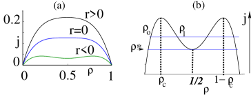
Figure 2: (a) Current versus $\rho$ for three values of $r$. (b) shows the notations used for $r<0$. The peak densities are $\rho_{c}$ and $1-\rho_{c}$. The inner layer connects pairs of densities (with same current) from $\rho_{o},\rho_{1},1-\rho_{1},1-\rho_{o}$. For $\rho_{1}=1/2$, the low and high densities are $\rho^{*}$ and $1-\rho^{*}$. For currents les than $j(1/2)$ (and also for $r\geq 0$), $\rho_{o}$ and $1-\rho_{o}$ are the two relevant densities.

The hydrodynamic approach based on the continuity equation with $j(\rho)$ of the conserved case is known to agree remarkably with numerical simulationshager ; popkov . In this approach the density satisfies a continuity equation supplemented by an additional contribution from the nonconserving process. The density then satisfies

$$\frac{\partial\rho}{\partial t}+\frac{\partial J}{\partial x}+S_{0}=0,$$ (3)

where $J$ is the current consisting of the bulk current $j(\rho)$ and a diffusive current, and

$$S_{0}(\rho)=-\Omega(\rho_{\rm L}-\rho),\quad\Omega=(\omega_{a}+\omega_{d})N,$$ (4)

accounts for the Langmuir dynamics. $\Omega$ is related to the net flux of particles and $\rho_{\rm L}$ is the density defined in Eq. 1. Nonconservation would matter only when the net flux of particles adsorbed or desorbed is comparable to the current in the system. For this reason $\Omega$ is kept constant, finite (scaling limit) for $N\to\infty$. By adding the diffusive (Fick’s law) current, $J$ in Eq. 3 can be written as

$$J=-\epsilon\frac{\partial\rho}{\partial x}+j(\rho),$$ (5)

with the diffusion constant $\epsilon\sim O(1/N)$ is a small parameter (not to be confused with $\varepsilon$), and is a remnant of the underlying lattice. This form, Eq. 5, also follows from a continuum limit of the discrete model. Despite its smallness $\epsilon$ plays an important role in the phase transitions, especially in shock formation. The steady state density profile is now given by

$$-\epsilon\frac{{\rm d}^{2}\rho}{{\rm d}x^{2}}+S_{1}(\rho)\frac{{\rm d}\rho}{{\rm d}x}+S_{0}(\rho)=0,$$ (6a)

$${\rm where} S_{1}(\rho)=\frac{{\rm d}j(\rho)}{{\rm d}\rho},$$ (6b)

and the boundary conditions $\rho(0)=\alpha$, and $\rho(1)=\gamma$. We already noted that $\rho=1/2$ is a special density due to the particle-hole symmetry. To avoid extra complications arising from the accidental matching of densities, we take $\omega_{a}\neq\omega_{d}$ so that $\rho_{\rm L}\neq 1/2$. Such cases will be considered elsewhere.

Eq. 6a entails two length scales, (i) $x$ for the bulk and (ii) $\tilde{x}=(x-x_{0})/\epsilon$ which is significant in a thin region as $\epsilon\to 0$ around an appropriately chosen $x_{0}$. Eq. 6a does not depend on the choice of $x_{0}$. The separation of the two scales is used to develop a uniform approximation of the solution order by order in $\epsilon$. Here we restrict ourselves to the lowest order approximant. The bulk solution in terms of $x$ comes from the first order equation obtained with $\epsilon=0$ in Eq. 6a. This solution, to be called the outer solution,

$$\rho(x)=\rho_{\rm out}(x)$$ (7)

is given implicitly by

$$g_{r}(\rho)=2\Omega\ x+C,$$ (8a)

where $$C$$ is a constant to be fixed by only one of the two boundary conditions, and

$$g_{r}(\rho) \equiv (uY^{2}_{\rm L}+r)\>Y+\frac{u}{2}Y_{\rm L}Y^{2}+\frac{u}{3}Y^{3}$$ (8b)

$$\qquad+(uY^{2}_{\rm L}+r)Y_{\rm L}\ln\mid Y_{\rm L}-Y\mid$$

with $Y=2\rho-1$,and $Y_{L}=2\rho_{L}-1$. We shall suppress the $r$-dependence in $g_{r}$, unless required. For the left boundary condition, the outer solution is

$$g(\rho)=2\Omega\ x+g(\alpha),$$ (9)

with a density

$$\rho_{o}\equiv\rho_{\rm out}(1)\ {\rm at}\ x=1,$$ (10)

determined by

$$g(\rho_{o})=2\Omega+g(\alpha).$$ (11)

Here, $\rho_{o}$ depends on $\alpha$, but in general, $\rho_{o}\neq\gamma$.

To satisfy the other boundary condition $\rho=\gamma$ at $x=1$, we use the second scale ${\tilde{x}}=(x-1)/\epsilon$ around the boundary point $x=1$. With this variable, the density (to be called the inner solution) satisfies

$$-\frac{{\rm d}^{2}\rho_{\rm in}}{{\rm d}\tilde{x}^{2}}+S_{1}(\rho_{\rm in})\frac{{\rm d}\rho_{\rm in}}{{\rm d}\tilde{x}}=0,$$ (12)

obtained from Eq. (6a) by first changing the variable to ${\tilde{x}}$ and then taking $\epsilon\to 0$. The absence of the $S_{0}$ term can be understood from the observation that for a constant $\Omega$ this layer is too thin for the nonconservation to matter, at least to leading order in $\epsilon$. For a smooth density profile (the solution of the second order equation with any $\epsilon>0$ no matter how small), we need to match the outer and the inner solutions by requiring that

$$\lim_{x\to 1}\rho_{\rm out}(x)=\lim_{\tilde{x}\to-\infty}\rho_{\rm in}(\tilde{x}).$$ (13)

Here ${\tilde{x}\to-\infty}$ gives the outer limit of the inner solution. Incorporating this matching condition, Eq. 12 can be written as

$$\frac{{\rm d}\rho_{\rm in}}{{\rm d}\tilde{x}}=j(\rho_{\rm in})-j(\rho_{o}),$$ (14)

in the thin boundary layer, with $\rho_{\rm in}(\tilde{x}=0)=\gamma$. The complete matched solution is obtained by joining the inner and outer approximations and subtracting their common value. Therefore, the density profile is given by

$$\rho(x)=\rho_{\rm out}(x)-\rho_{o}+\rho_{\rm in}(\tilde{x})+O(\epsilon).$$ (15)

Eq. 15 identifies the scale dependent separation of the bulk and the boundary contributions and it provides a uniform approximation of the density in the whole domain including the boundaries.

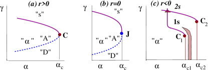
Figure 3: Schematic diagram of the phase boundary for shock at $x=1$. Thin, thick and dotted lines represent continuous transitions, first order transitions and dual lines respectively. “A”[“D”]: accumulated [depleted] bounary layer. C, C₁, C₂ are the critical points and J the tricritical point. “$\alpha$” and “s” represent $\alpha$-phase and shock phase with 1,2 denoting 1-shock, 2-shock phases. The phase boundary separating the $\alpha$ and the 1s phases is given by Eq. (20). Downward shocks appear in the hatched region (with $\gamma\leq 1/2$) in (c). The dual lines demarcating “A”/“D” are not shown in (c).

Let us first consider the $r>0$ case. The current has only one peak at $\rho=1/2$. The transport across the track is analogous to the well-understood ASEP case. For a low injection rate $\alpha$, the bulk density profile does not depend significantly on the withdrawal rate so long $\gamma$, the accumulated density at $x=1$, is small. One gets the $\alpha$-phase. For low $\gamma$, there is a depletion layer at $x=1$, which changes for $\gamma>\gamma_{d}\equiv\rho_{o}(\alpha)$ to an accumulated layer. This is the dual boundary transition mentioned earlier. By symmetry (Fig. 2) and from Eq. (14), $\rho_{\rm in}(\tilde{x})$ would saturate at $\rho=1-\rho_{o}(\alpha)$ as ${\tilde{x}}\to\infty$. Consequently, for $\gamma\geq\gamma_{s}\equiv 1-\rho_{o}(\alpha)$, a boundary layer given by Eq. (14) is not sufficient to satisfy the boundary condition at $x=1$. In this situation, the density profile is given by the two outer solutions,

$$g(\rho_{\rm rgt})=2\Omega\ (x-1)+g(\gamma)$$

on the right side and

$$g(\rho_{\rm lft})=2\Omega\ x+g(\alpha)$$

on the left. These two solutions are joined smoothly in a thin region by the inner solution of Eq. (12) with ${\tilde{x}}=(x-x_{s})/\epsilon$. On the bulk scale this looks like a discontinuity and is therefore a shock at $x=x_{s}$. The matching conditions and the location of the shock ($x_{s}$) are given by

$$\rho_{\rm lft}(x\to x_{s}-) = \lim_{\tilde{x}\to-\infty}\rho_{\rm in}(\tilde{x}),$$ (16a)

$${\rm and}\quad\rho_{\rm rgt}(x\to x_{s}+) = \lim_{\tilde{x}\to\infty}\rho_{\rm in}(\tilde{x}),$$ (16b)

where Eq. 16a is the matching of the left outer solution to the left end of the inner solution while Eq. 16b is the matching for the right side. This deconfinement of the boundary layer by shifting into the bulk as a shock is the shockening transition. For a given $\alpha$, the shock and the dual transitions are given by

$$\gamma = \gamma_{s}\equiv 1-\rho_{o}(\alpha)\qquad{\rm(shockening)}$$ (17)

$$\gamma = \gamma_{d}\equiv\rho_{o}(\alpha)\qquad{\rm(dual)}$$ (18)

The critical point $(\alpha_{c},\gamma_{c})$, being the point of intersection of the two lines, has $\gamma_{c}=1/2$, and $\alpha_{c}$ satisfying Eq. (11) with $\rho_{o}=\gamma_{c}$.

The shape of the transition curve near $(\alpha_{c},\gamma_{c})$ for any $r>0$ follows from Eq. (11), by noting that $dg(\rho)/d\rho$ is zero at $\rho=\gamma_{c}$ but not at $\rho=\alpha_{c}$. This shows that the shape exponent $\chi$ is given bysmsmb

$$\gamma-\gamma_{c}\sim\mid\alpha-\alpha_{c}\mid^{\chi},\quad{\rm with}\ \chi=1/2,$$ (19)

close to the critical point. The phase diagram is shown in Fig. 3a. The critical point $(\alpha_{c}(r),\gamma_{c})$ changes with $r$ but the exponents remain the same as in the ASEP case. We note in passing that for $\gamma<\gamma_{c}$, one crosses the dual phase boundary so that there is a depletion layer near $x=1$. This layer is non-shockening in the sense that it never reaches saturationsmvm ; smb_jpa07 . It acts as a shield for the boundary density, rendering the “effective” boundary condition at $x=1$ as $\gamma=\gamma_{c}$. Consequently, thanks to this depletion layer, there is a continuation of the critical point in the phase diagram.

The situation is completely different for $r<0$. We refer to Fig. 2). Let us start with small injection rates. There is a dual line at $\gamma=\rho_{o}(\alpha)$ so long $\rho_{o}(\alpha)<\rho^{*}$ (Fig. 2). There will be a symmetric shock centered around $\rho=1/2$. The transition to the shock phase (or the shockening transition) is at $\gamma=\gamma_{s}\equiv 1-\rho_{o}(\alpha)$. However, with change of $\alpha$ when $\rho_{o}$ exceeds $\rho^{*}$, the boundary layer bridges $\rho_{o}$ to $\rho_{1}<1/2$. The dual line continues to be $\gamma=\gamma_{d}=\rho_{o}(\alpha)$, but the shock line is given by

$$\gamma=\gamma_{s1}\equiv\rho_{1}(\alpha).$$ (20)

The shock is therefore smaller in height, lying below $\rho=1/2$. A zero height shock at the boundary is now possible if the following two conditions are met: (i) the injection rate $\alpha$ is such that the outer solution gives the peak density at the boundary, i.e., $\rho_{o}(\alpha)=\rho_{c}$, and (ii) the withdrawal rate is such that the accumulated density $\gamma$ is also $\rho_{c}$. Under these conditions, the density will then have an infinite slope at the $x=1$ boundary. Therefore, $\gamma=\rho_{c}=\rho_{o}(\alpha)$ gives a critical point. This locates an off-center critical point C₁ in Fig 3c, with

$$\gamma_{c1}=\rho_{c}\ {\rm and}\ \alpha=\alpha_{c1},$$ (21)

where $\alpha_{c1}$ satisfies Eq. 11 with $\rho_{o}=\gamma_{c1}$.

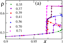
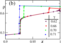
Figure 4: Plots of $\rho(x)$ vs. $x$ ($r=-0.2,u=2.2,\Omega=0.1$) from numerical solution. The values of $\gamma$ are indicated on the plots while $\alpha$ is kept fixed, close to $\alpha_{c1}$ in (a) and $\alpha_{c2}$ in (b). In (a), as $\gamma$ increases, one sees a sequence: (i) the shock developing from zero height ($\gamma=0.35$) to a maximum ($\gamma=0.39$), (ii) an additional downward shock ($\gamma=0.41$) which goes towards the boundary ($\gamma=0.56$), (iii) the emergence of another upward shock of finite height ($\gamma=0.70$) , and (iv) finally a bigger shock symmetric around $\rho=1/2$ ($\gamma=0.71$). (b) shows the sequence for the second critical point. There is no downward shock here, while the first shock is of maximum possible height. To be noted is the depletion layer for $\gamma=0.62$.

The density profile close to this critical point $C_{1}$ (for $r<0$) is shown in Fig. 4a. These are obtained by a numerical solution of Eq. (6a) in the limit of small $\epsilon$. For $\frac{1}{2}>\gamma>\gamma_{c1}$, the shock height starts increasing with $\gamma$ until the shock connects $\rho=\rho^{*}$ and $\rho=1/2$. This is the largest shock one can produce from the left peak of the current. For a range of $\gamma$ there is the possibility of a downward shock. One sees an overcrowded region sandwiched between the $\alpha$-phase and the $\gamma$-phase, even though both $\alpha$ and $\gamma$ are less than $1/2$, but the shock is centered around $1/2$. The downward shock shifts towards $x=1$ as $\gamma$ is changed and it disappears as it hits the boundary. At this point the downward shock gets converted into a depleted boundary layer. With increase in $\gamma$, the depleted layer undergoes a boundary transition to an accumulated layer leading to a second shock from the second peak. There is no obvious symmetry relation between the two upward shocks except for their centers. The sequence is shown in Fig. 4a. For $\gamma>1-\rho^{*}$, the two shocks merge into one bigger one centered around $\rho=1/2$.

Next, consider $\alpha>\alpha_{c1}$ as shown in Fig. 4b. With the largest shock from the low density peak of the current, it is possible for the density to reach the second peak of the current, $\rho=1-\rho_{c}$, at $x=1$. This gives the second critical point because the shock height starts from zero as $\gamma$ exceeds $1-\rho_{c}$. The second critical point C₂ at $(\alpha_{c2},\gamma_{c2})$ is determined by

$$\gamma_{c2} = 1-\rho_{c},$$ (22a)

$$g(\gamma_{c2}) = 2\Omega\ (1-x_{s})+g(0),$$ (22b)

$$g(0) = 2\Omega\ x_{s}+g(\alpha_{c2}),$$ (22c)

where $x_{s}$ is the position of the first shock, and $g$ is from Eq. (9) with $r<0$. Fig. 3c shows the nature of the phase boundary for a given value of $r<0$. These two critical points $C_{1},C_{2}$ merge as $r\to 0$. Given the form of $g(\rho)$ in Eq. (8b), we find

$$\mid\gamma_{c1}-\gamma_{J}\!\mid\;\sim\;\mid\gamma_{c2}-\gamma_{J}\!\mid\;\sim\;{\mid\!r\!\mid}^{1/2},\ (r\to 0-),$$ (23)

where $\gamma_{\rm J}$ is the critical value at $r=0$. The power law dependence is expected to be universal. The bifurcation at point J is shown in Fig. 1a in the projected plane of $\gamma$-$r$. The full three dimensional lines are shown in Fig. 1b. An analysis as done for the $r>0$ case shows that the shape of the boundaries at these new critical points would be similar to that for the $r>0$ case, i.e the shape exponent will be $\chi=1/2$ as in Eq. (19), implying universality.

Let us now consider the special point J. The physical picture developed above remains valid here. The tricritical point J, being at the intersection of the shock line and the dual line, is at

$$g_{r=0}(\gamma_{\rm J})=2\Omega+g_{r=0}(\alpha_{\rm J}),\quad\gamma_{\rm J}=1/2.$$ (24)

Since $S_{1}(\rho)\sim(\rho-1/2)^{3}$, the shape exponent is

$$\chi_{\rm J}=1/4,$$ (25)

where $\chi_{\rm J}$ is defined as

$$\gamma-\gamma_{\rm J}\sim\mid\alpha-\alpha_{\rm J}\mid^{\chi_{\rm J}}.$$ (26)

The phase boundary is shown in Fig. 3b. The first order transition lines as shown in Fig. 3 become surfaces in the three dimensional phase diagram. These first-order surfaces end on critical lines and these critical lines are shown in Fig. 1b. The locus of the intersection of the first order lines for $r<0$ (triangle in Fig 3c) in the extended phase diagram is a line ending at J. This is the line on which both the shocks connecting $\rho=\rho^{*}$ to $\rho=1/2$ and $\rho=1/2$ to $\rho=1-\rho^{*}$ are just at $x=1$. This completes the identification of J as the tricritical point where a first order line is converted into a continuous one.

The crossover from the tricritical to the critical behaviour is obtained by expanding Eq. 11 around $\alpha=\alpha_{J},\rho_{o}=\gamma_{J}$ and $r\to 0+$. The shape of the transition curves and also the height of the shocks near the tricritical point can be described by a scaling form

$$\alpha-\alpha_{\rm J}\sim\;\mid\!\gamma-\gamma_{\rm J}\!\mid^{1/\chi_{\rm J}}\ {\cal F}\left({r}\;{\mid\!\gamma-\gamma_{\rm J}\!\mid^{-\psi_{\rm J}}}\right),$$ (27)

where ${\cal F}(x)$ is a scaling function with the crossover exponent $\psi_{\rm J}=2$. For $x\to 0$, ${\cal F}(x)\to$ constant while for large $x$, ${\cal F}(x)\sim x$. For $r\neq 0$, with $\gamma$ close to the critical value, the scaling variable becomes large and one recovers the critical value $\chi^{-1}=\chi^{-1}_{\rm J}-\psi_{\rm J}=2$. This also shows the importance of the tricritical point because it controls the scaling behaviour in its neighbourhood.

Within the window of the single shock phase for $r<0$, there is a region of downward shock bounded by critical and first order lines. The peculiarity of the downward shock is that it does not traverse the whole lattice but goes critical within the track. The thickness of the region in the phase diagram is determined by the shallowness of the minimum at $\rho=1/2$. Details of these lines and the region will be reported elsewhere.

In summary, we have shown that the repulsive interaction induced particle-hole symmetry breaking in the form of a double peaked current in one dimensional asymmetric exclusion process leads to a nonequilibrium tricritical point. This tricritical point controls the scaling behaviour in its neighbourhood. The tricritical exponents are different from the critical ones and an additional crossover exponent is required for the crossover to the critical behaviour. The phase diagram also shows a region of downward shock. It remains to be seen if this is a necessity for the nonequilibrium tricriticality.

- (1) email: jayamaji@iopb.res.in; somen@iopb.res.in
- (2) B. Derrida et. al., J. Phys. A 26 (1993) 1493; G. Schütz and E. Domany, J. Stat. Phys. 72 (1993) 277.
- (3) A. Parmeggiani, T. Franosch and E. Frey, Phys. Rev. Lett. 90 (2003) 086601; Phys. Rev. E 70 (2004) 046101.
- (4) M. R. Evans, R. Juhasz and L. Santen, Phys. Rev. E 68 (2003) 026117.
- (5) S. Mukherji and S. M. Bhattacharjee, J. Phys. A 38 (2005) L285.
- (6) S. Mukherji and V. Mishra, Phys. Rev. E 74 (2006) 011116.
- (7) K. Huang, Statistical Mechanics, (John Wiley, NY) 1987.
- (8) A. Aharony in Critical Phenomena, Ed. by F. J. W. Hahne (Springer, Berlin) 1983.
- (9) M. Acharyya, Phys. Rev. E 59 (1999) 218; G. Korniss et. al., Phys. Rev. E 66 (2002) 056127; L. Giada and M. Marsili, Phys. Rev. E 62 (2000) 6015 ; H. K. Jenssen et. al., Phys. Rev. E 70 (2004) 026114. A. Antoniazzi, D. Fanelli, S. Ruffo, and Y. Y. Yamaguchi Phys. Rev. Lett. 99 (2007) 040601.
- (10) P. G. de Gennes, Scaling Concepts in Polymer Physics, (Cornell U. Press, Ithacar) 1979.
- (11) S. M. Bhattacharjee, Phys. Rev. Lett 76 (1996) 4568. S. M. Bhattacharjee and S. Mukherji, Phys. Rev. Lett. 83 (1999) 2374;
- (12) M. Stephanov, Prog. Theo. Phys. Suppl. No. 153 (2004) 139.
- (13) J. S. Hager et. al., Phys. Rev. E 63 (2001) 056110. S. Katz, J. Lebowitz, and H. Spohn, J. Stat. Phys. 34 (1984) 497.
- (14) J. Krug, Phys. Rev. Lett. 67 (1991) 1882
- (15) V. Popkov et. al., Phys. Rev. E 67 (2003) 066117.
- (16) M. Arabsalmani and A. Aghamohammadi, Eur. Phys. J. B55, (2007) 439
- (17) S. Mukherji, Phys. Rev. E 76 (2007) 011127.
- (18) S. M. Bhattacharjee, J. Phys. A: Math. Theor. 40 (2007) 1703.