Effective Field Theory of Triangular-Lattice Three-Spin Interaction Model

Abstract

We discuss an effective field theory of a triangular-lattice three-spin interaction model defined by the ${\mathbb{Z}}_{p}$ variables. Based on the symmetry properties and the ideal-state graph concept, we show that the vector dual sine-Gordon model describes the long-distance properties for $p\geq 5$; we then compare its predictions with the previous argument. To provide the evidences, we numerically analyze the eigenvalue structure of the transfer matrix for $p=6$, and we check the criticality with the central charge $c=2$ of the intermediate phase and the quantization condition of the vector charges.

The XY model consisting of the inner products of two neighboring planar spins with the ${\mathbb{Z}}_{p}$ symmetry-breaking field has been extensively researched; it provides the basic understanding of more complicated models and also of real materials. Especially, for the two-dimensional (2D) case, the effective theory for the long-distance behaviors was established based on the 2D Coulomb gas (CG) picture and the renormalization-group (RG) concepts, thereby enabling its complete understanding.[1] In this paper, we investigate its extension, i.e., the three-spin interaction model (TSIM) that was introduced a long time ago by Alcaraz et al.[2, 3] Suppose that $\langle k,l,m\rangle$ denotes three sites at the corners of each elementary plaquette of the triangular lattice $\Lambda$ (consisting of interpenetrating sublattices $\Lambda_{\rm a}$, $\Lambda_{\rm b}$, and $\Lambda_{\rm c}$), then the following reduced Hamiltonian expresses a class of TSIM:

$${\cal H}=-\beta J\sum_{\langle k,l,m\rangle}\cos\left(\varphi_{k}+\varphi_{l}+\varphi_{m}\right).$$ (1)

Angle $\varphi_{k}=2\pi n_{k}/p$, $n_{k}\in[0,p-1]$ defines the ${\mathbb{Z}}_{p}$ variable. For $p=2$, eq. (1) is the exactly solved Baxter-Wu model with three-spin-product interactions,[4] but for larger $p$, it becomes puzzling in its expression in terms of the spin variables. However, for $p\geq 5$ on which we will concentrate, its effective theory possesses a remarkably simple structure and can provide a unified understanding in a wide area of researches, including those on the 2D melting phenomena. Therefore, our aim is to formulate it based on a recent approach and to confirm its predictions quantitatively via numerical calculations.

We shall begin with the symmetry properties. Adding to the translations and space inversions, the model is invariant under the global spin rotations: $\varphi_{k}\mapsto\varphi_{k}+\sum_{\rho={\rm a,b,c}}\sum_{l\in\Lambda_{\rho}}(2\pi n_{\rho}/p)\delta_{k,l},$ if the sublattice dependent numbers satisfy a condition $n_{\rm a}+n_{\rm b}+n_{\rm c}=0$ (mod $p$).[2, 3] This symmetry operation—denoted as $(n_{\rm a},n_{\rm b},n_{\rm c})$—can be generated from two of the three fundamental operations with the following minimal spin rotations:

$$\hat{R}_{\rm a}\!:(1,p-1,0),~{}\hat{R}_{\rm b}\!:(0,1,p-1),~{}\hat{R}_{\rm c}\!:(p-1,0,1).$$ (2)

Here, note that these commuting operations satisfy some relations, e.g., $\hat{R}_{\rm a}^{p}=\hat{R}_{\rm c}\hat{R}_{\rm b}\hat{R}_{\rm a}=\hat{1}$ (identity operation). At a sufficiently low temperature, this symmetry can be broken due to the three-spin interaction, and one of the ordered states is stabilized. An obvious one is $\{\varphi_{k}\}=0$, and the others can be obtained by successively applying eq. (2). Consequently, we can observe a $p^{2}$-fold degeneracy corresponding to the order of the group.[2, 3]

Here, we shall mention that our strategy to formulate the effective field theory is based on the recent development by Kondev and Henley,[5, 6] where the critical ground states of various 2D classical systems have been treated in a unified way. So, to make it concrete, let us consider the structure of the so-called ideal-state graph $\cal I$ for the present problem. We expect that, like the flat states in the interface models, the above $p^{2}$ ordered states should be specified by the locking points of a certain kind of field variable; thus, the dimension and the structure of ${\cal I}$ determine the number of components and the compactification region of the fields, respectively. By definition, each node of $\cal I$ represents one of the ordered states, and each link exhibits the neighboring two nodes connected by minimal spin rotations. From the above-mentioned symmetry properties, there are two commuting generators, so the graph is located in a 2D space. Further, due to relations such as $\hat{R}_{\rm c}\hat{R}_{\rm b}\hat{R}_{\rm a}=\hat{1}$, the shortest loop of links should form the triangle. These require $\cal I$ to be defined on the triangular lattice. On one hand, for a given value of $p$, the periodicity conditions, e.g., $\hat{R}_{\rm a}^{p}=\hat{1}$, define the unit cell of the so-called repeat lattice $\cal R$. From these, we can obtain ${\cal I}$. In Fig. 1, we give an example for $p=6$, where 36 ideal states are specified by the sublattice dependent numbers $n_{\rm a}$, $n_{\rm b}$, and $n_{\rm c}$ (e.g., “000” at the corners represents $\{\varphi_{k}\}=0$).

A two-component field theory is clarified to be relevant to the present model in its continuum limit; we shall write it as ${\bf\Phi}({\bf x})\in{\mathbb{R}}^{2}$ (${\bf x}$ is the 2D real-space position vector). It then satisfies the periodicity conditions ${\bf\Phi}\equiv{\bf\Phi}+2\pi{\bf e}_{\alpha}$, where $\{{\bf e}_{\alpha}\}~{}(\alpha=1,2)$ denote the normalized (non-orthogonal) fundamental lattice vectors of $\cal R$ (see Fig. 2). For the representations of the physical quantities in terms of ${\bf\Phi}$, it is also important to see the relationship between the discrete symmetry operations for spins and the field transformations, ${\bf\Phi}\mapsto{\bf\Phi}+\delta{\bf\Phi}$; especially, the correspondence of the minimal spin rotations eq. (2) to the following $\delta{\bf\Phi}$ (see the inset of Fig. 1):

$$\hat{R}_{\rm a}\!:\frac{2\pi}{p}{\bf e}_{1},~{}\hat{R}_{\rm b}\!:-\frac{2\pi}{p}{\bf e}_{1}+\frac{2\pi}{p}{\bf e}_{2},~{}\hat{R}_{\rm c}\!:-\frac{2\pi}{p}{\bf e}_{2},$$ (3)

which retain relations, e.g., $\hat{R}_{\rm c}\hat{R}_{\rm b}\hat{R}_{\rm a}=\hat{1}$. Our next task is to derive the Lagrangian density by which the low-energy and long-distance behaviors can be captured. For this purpose, we shall first focus on the low-temperature region, at which the relevant potential may perturb the kinetic energy part representing the spatial fluctuation of ${\bf\Phi}({\bf x})$. As we shall see, the latter is also responsible for the description of the intermediate critical phase.[2, 3]

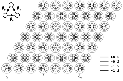
Figure 1: The ideal-state graph ${\cal I}$ for $p=6$. Triplets of numbers exhibit 36 ordered states. The contour plot of the locking potential and the transformation eq. (3) (inset) are also given.

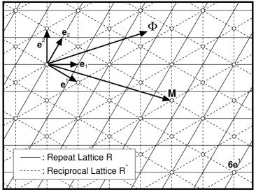
Figure 2: The repeat lattice ${\cal R}$ and its reciprocal lattice ${\cal R}^{*}$. The fundermental lattice vectors are also given by arrows.

Due to the periodicity of ${\bf\Phi}$, the vector charge $\bf M$ is quantized to take the values on the reciprocal lattice of $\cal R$, ${\cal R}^{*}$ (Fig. 2). Then, the local densities relating to the spin degrees of freedom may be expanded to the Fourier series by using the vertex operators as $Q({\bf\Phi})=\sum_{{\bf M}\in{\cal R^{*}}}h_{{\bf M}}{\rm e^{i{\bf M\cdot\Phi}}}$. While the inner-product form ensures a coordinate invariance in ${\mathbb{R}}^{2}$, we look into its expression by using their elements to get some familiarity. Writing the reciprocal lattice vectors as $\{{\bf e}^{\alpha}\}~{}(\alpha=1,2)$, the inner product between ${\bf M}=m_{\alpha}{\bf e}^{\alpha}$ and ${\bf\Phi}=\sqrt{2}\phi^{\alpha}{\bf e}_{\alpha}$ becomes $\sqrt{2}m_{\alpha}\phi^{\alpha}$, where the covariant and contravariant elements satisfy $m_{\alpha}\in{\mathbb{Z}}$ and $\sqrt{2}\phi^{\alpha}\equiv\sqrt{2}\phi^{\alpha}+2\pi$, respectively (the summation convention is used and the factor $\sqrt{2}$ is for later convenience), since $\{{\bf e}_{\alpha}\}$ and $\{{\bf e}^{\alpha}\}$ are dual (i.e., ${\bf e}_{\alpha}\cdot{\bf e}^{\beta}=\delta_{\alpha}^{\beta}$). Also, the norm of ${\bf M}$, for example, is given by $\|{\bf M}\|=\sqrt{m_{\alpha}m^{\alpha}}$, where the metric tensor is defined by $g^{\alpha\beta}\equiv{\bf e}^{\alpha}\cdot{\bf e}^{\beta}$ and the contravariant elements by $m^{\alpha}\equiv g^{\alpha\beta}m_{\beta}$, as usual.[7]

To obtain an explicit form of the locking potential, the following three issues need to be addressed:[5, 6] (i) Since the potential is a part of the Lagrangian density, it should be invariant under eq. (3). (ii) It is sufficient to keep the most relevant terms in the RG sense. Since the dimension of a vertex operator is proportional to the squared norm of its vector charge (see below), it is sufficient to keep those with the shortest ones. (iii) The point group symmetry of the triangular lattice for ${\cal I}$, which stems from the sublattice and the spin-rotational symmetries, should be taken into account. Consequently, these requirements can be realized as the expression $V({\bf\Phi})=h_{p}\sum_{\|{\bf M}\|=pa^{*}}{\rm e^{i{\bf M\cdot\Phi}}}$, where $a^{*}\equiv\sqrt{g^{11}}$ and $h_{p}$ are the lattice constant of ${\cal R}^{*}$ and the coupling constant, respectively. The summation is over the following six vectors: $\pm p{\bf e}^{1}$, $\pm p{\bf e}^{2}$, and $\pm p({\bf e}^{1}+{\bf e}^{2})$. In Fig. 1, we give the contour plot of $V({\bf\Phi})$ for $p=6$ and $h_{6}=1/2$; we observe that the points with the minimum value form the triangular lattice and each point corresponds to the ideal state.

While the locking point specifies the ordered state, the spatial fluctuation of the fields becomes important with the increase of the temperature. For $p\geq 5$, the critical intermediate phase is expected,[2, 3] and it must correspond to the roughing phase of an interface model.[8] Thus, we can safely introduce the free-boson Lagrangian density for the fluctuations:

$${\cal L}_{0}[{\bf\Phi}]=\frac{K}{2\pi}\partial_{i}\phi_{\alpha}\partial_{i}\phi^{\alpha},$$ (4)

where $g_{\alpha\beta}\equiv{\bf e}_{\alpha}\cdot{\bf e}_{\beta}$ and $\phi_{\alpha}\equiv g_{\alpha\beta}\phi^{\beta}$. The Gaussian coupling $K$ plays the role of inverse temperature to control the stiffness of the interface. The summation over $i$ $(=x,y)$ specifying the Cartesian component of ${\bf x}$ in the basal 2D plain is also assumed.

At this stage, ${\cal L}_{0}+{\cal L}_{1}$ with

$${\cal L}_{1}[{\bf\Phi}]=\frac{y_{p,0}}{2\pi\alpha_{0}^{2}}\sum_{\|{\bf M}\|=pa^{*}}{\rm e^{i{\bf M\cdot\Phi}}}$$ (5)

($y_{p,0}\propto h_{p}$ and $\alpha_{0}$ is the cutoff of $\Lambda$) can describe the lower temperature transition to the ordered phase. On the other hand, for the transition to the disordered phase, we should next consider the discontinuity of ${\bf\Phi}$ by an amount of $2\pi{\bf N}$ (${\bf N}\in{\cal R}$), which becomes frequent with the increase of the temperature. This topological defect is created by the vertex operator ${\rm e^{i{\bf N\cdot\Theta}}}$, where ${\bf\Theta}$ is the dual field of ${\bf\Phi}$ and is defined as $K\partial_{i}{\bf\Phi}=\epsilon_{ij}\partial_{j}{\bf\Theta}$ ($\epsilon_{ij}$ is the antisymmetric symbol). ${\cal L}_{0}$ is invariant under the transformation, $K\leftrightarrow 1/K$ and ${\bf\Phi}\leftrightarrow{\bf\Theta}$, so the stiffness of the interface described by ${\bf\Theta}$ becomes larger with the increase of the temperature. Therefore, the potential can become relevant to bring about a unique flat state corresponding to the disordered phase. If we write ${\bf\Theta}\equiv\sqrt{2}\theta_{\alpha}{\bf e}^{\alpha}$, then the covariant elements satisfy $\sqrt{2}\theta_{\alpha}=\sqrt{2}\theta_{\alpha}+2\pi$, because the vector charge ${\bf N}$ is in ${\cal R}$. To obtain the explicit form of the locking potential, we can repeat the same argument as before, and arrive at the following form:

$${\cal L}_{2}[{\bf\Theta}]=\frac{y_{0,1}}{2\pi\alpha_{0}^{2}}\sum_{\|{\bf N}\|=1}{\rm e^{i{\bf N\cdot\Theta}}},$$ (6)

which gives the extremum on the lattice points of ${\cal R}^{*}$. Consequently, we see that the vector dual sine-Gordon field theory ${\cal L}\equiv{\cal L}_{0}+{\cal L}_{1}+{\cal L}_{2}$ provides an effective description of TSIM. In the remaining part of this letter, we shall check our prediction analytically and numerically. Here, we summarize the scaling dimensions of the operators on ${\cal L}_{0}$. The vertex operator with the electric and magnetic vector charges $({\bf M,N})$ is defined as $O_{\bf M,N}\equiv{\rm e}^{{\rm i}({\bf M\cdot\Phi}+{\bf N\cdot\Theta})}$, which has the dimension $x_{\bf M,N}\equiv\frac{1}{2}(K^{-1}\|{\bf M}\|^{2}+K\|{\bf N}\|^{2})$. This formula supports our treatment that the vertex operators with the shortest vector charges were kept in the effective theory. In addition, the bosonized expression of the spin degrees of freedom, $S_{k}\equiv{\rm e}^{{\rm i}\varphi_{k}}$, is also important. It only contains the electric charges and should reproduce eq. (2) on applying eq. (3). We can see that the sublattice dependent expression, $(S_{\rm a},S_{\rm b},S_{\rm c})=(O_{{\bf e}^{1}+{\bf e}^{2},{\bf 0}},O_{-{\bf e}^{1},{\bf 0}},O_{-{\bf e}^{2},{\bf 0}})$, satisfies the requirement and reproduces the ordered-state spin configurations on ${\cal I}$. Furthermore, these exhibit that the condition to give nonvanishing spin correlations [2, 3] is reduced to that of the vector charge neutrality.[9] For instance, since the two-spin (three-spin) product $S_{\rho}({\bf x})S^{*}_{\sigma}({\bf y})$ $[S_{\rho}({\bf x})S_{\sigma}({\bf y})S_{\tau}({\bf z})]$ becomes neutral for $\rho=\sigma$ ($\rho\neq\sigma\neq\tau\neq\rho$), the average with respect to ${\cal L}_{0}$ takes a nonzero value only between the same sublattice (among different sublattices).

Now, we are in a position to discuss the transitions. Although the free part ${\cal L}_{0}$ is perturbed by ${\cal L}_{1,2}$ (dimensions are $x_{y_{p,0}}=2p^{2}/3K$ and $x_{y_{0,1}}=K/2$), these are both irrelevant for $p^{2}/3\geq K\geq 4$. To obtain the lower and higher temperature transition points (say $T_{\rm L,H}$), we should resort to the numerical calculations, but these are considered to correspond to the above terminuses. Thus, let us first focus on the region near $T_{\rm H}$ where ${\cal L}_{1}$ is irrelevant. Instead of performing the perturbative RG calculation ($\alpha_{0}\to\alpha_{0}{\rm e}^{{\rm d}l}$), we shall see that our problem can be related to the works by Halperin, Nelson, and Young,[10, 11, 12, 13] where the defect-mediated 2D meltings were studied based on the Kosterlitz-Thouless (KT) RG argument [9] (the so-called KTHNY theory). In fact, Alcaraz et al., making use of the vector CG representation with the long-range interaction, pointed out the relevance to 2D melting via the dissociation of dislocation pairs without the angular force. While our Lagrangian density ${\cal L}_{0}+{\cal L}_{2}$ is in the local representation, we can also find its counterpart in ref. Nels78. Therefore, we confirm their assertion, and we shall discuss the transition in detail. As the Burgers vector characterizes the dislocation for the triangular lattice, ${\bf N}$ in eq. (6) takes the six vectors, $\pm{\bf e}_{1}$, $\pm{\bf e}_{2}$, and $\pm({\bf e}_{1}-{\bf e}_{2})$, so the three-point function of the local density ${\cal L}_{2}$ provides a nonvanishing value owing to the satisfaction of the neutrality condition. This results in a nonzero operator-product-expansion (OPE) coefficient among them; it yields the $y_{0,1}^{2}(l)$ term in the $\beta$-function for the coupling constant $y_{0,1}(l)$ (the fugacity for dislocations), while that for $x(l)\equiv 2-x_{y_{0,1}}(l)$ basically remains unchanged.[14] Consequently, we obtain the KT-like flow diagram (see Fig. 8 in ref. Nels78). For $T>T_{\rm H}$, the correlation length behaves as $\xi\propto{\rm exp}[C/(T-T_{\rm H})^{\frac{2}{5}}]$ characterizing the disordered phase, while for $T<T_{\rm H}$ the exponent of the spin correlation function varies as $\eta\equiv 2x_{S}=4/3K$ and $\eta_{\rm H}=1/3$ at $T_{\rm H}$ (without corrections).

Second, we shall discuss the region near $T_{\rm L}$ where ${\cal L}_{2}$ is irrelevant. While having seen the $p^{2}$ ordered states by ${\cal L}_{1}$, we can also find a similar type of transition in refs. Halp78 and NelsHalp79, where the transition from the “floating solid” to “commensurate solid” was discussed for the case that the substrate periodic potential is commensurate with the adsorbate lattice. Indeed, they observed its similarity to the dislocation-mediated melting. For the present model, Alcaraz et al. obtained the RG equations based on the duality observed in the vector CG representation.[2, 3] On the other hand, we can also reproduce them and also the finite $\xi$ for $T<T_{\rm L}$ and $\eta_{\rm L}=4/p^{2}$ at $T_{\rm L}$, etc, based on our local representation and OPE coefficients.

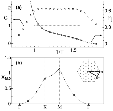
Figure 3: (a) $1/T$ vs. $c$ (circles) and $\eta$ (squares). (b) The ${\bf M}$ dependence of $x_{\bf M,0}$ at $1/T_{\rm SD}\simeq$1.252. Dotted curves exhibit $\|{\bf M}\|^{2}/2K$ with $K=4\sqrt{3}$ along the path in the inset.

To confirm the effective theory, we shall provide the numerical calculation results here. We consider the system on $\Lambda$ with $M$ ($\to\infty$) rows of $L$ (a multiple of 3) sites wrapped on the cylinder and define the transfer matrix connecting the next-nearest-neighbor rows. We denote its eigenvalues as $\lambda_{q}(L)$ or their logarithms as $E_{q}(L)=-\frac{1}{2}\ln|\lambda_{q}(L)|$ ($q$ specifies a level). Then, the conformal invariance provides the expressions of the central charge $c$ and the scaling dimension $x_{q}$ in the critical systems as $E_{\rm g}(L)\simeq Lf-{\pi}c/{6L\zeta}$ and $\Delta E_{q}(L)\simeq{2\pi}x_{q}/{L\zeta}$. Here, $E_{\rm g}(L)$, $\Delta E_{q}(L)$ $[=E_{q}(L)-E_{\rm g}(L)]$, $\zeta$ $(=2/\sqrt{3})$, and $f$ correspond to the ground-state energy, an excitation gap, the geometric factor, and a free energy density, respectively.[15, 16, 17] When performing the diagonalization calculations, we employ two of three spin rotations in eq. (2) [e.g., $(\hat{R}_{\rm a},\hat{R}_{\rm b})$] as well as the lattice translation and space inversion. This is because the matrix size can be reduced, and more importantly, discrete symmetries can specify lower-energy excitations. For instance, we can find the excitation level corresponding to the spin operator $S_{\rm a}({\bf x})$ in the sector with indexes $({\rm e}^{{\rm i}2\pi/p},1)$.

In the following, we give the results for $p=6$, which are obtained using the data up to $L=9$. In Fig. 3(a), we provide the $T$ dependence (in units of $J/k_{\rm B}$) of $c$ where the region keeping $c\simeq 2$ can be recognized. From this plot, we roughly estimate the KT-like transition temperatures as $1/T_{\rm L}\simeq 1.5$ and $1/T_{\rm H}\simeq 1.1$ (see also refs. Alca82 and Alca83). Next, we plot the $T$ dependence of $\eta$ along its second axis, which shows that $\eta$ is the increasing function of $T$ and takes close values to $\eta_{\rm L,H}=1/9$, 1/3 around the estimates of $T_{\rm L,H}$ (see dotted lines). In Fig. 3(b), we give the scaling dimension $x_{\bf M,0}$ as a function of the electric vector charge ${\bf M}$ along the path depicted in the inset. As a representative for the critical region, we pick up the self-dual point by numerically observing the level crossing, $x_{y_{6,0}}=x_{y_{0,1}}$; we then perform the calculations at $1/T_{\rm SD}\simeq 1.252$. From the figure, we can verify that the dimension depends only on the norm of the electric vector charge. Further, despite the treated $L$ being small—the size dependence is actually larger for those with longer vectors—the results (open circles) agree well with the theoretical formula (dotted curves), which quantitatively supports our above argument.

To summarize, based on the ideal-state graph approach by Kondev and Henley, we have discussed the effective field theory for TSIM. Due to the symmetry properties, two kinds of vector charges, ${\bf M}$ and ${\bf N}$, take the values of the reciprocal and repeat lattice points, and then provide the descriptions of the phase transitions. While the effective theory is given by the vector dual sine-Gordon model, we have seen its close relationship to the KTHNY theory, as pointed out by Alcaraz et al. We also performed numerical calculations to check some theoretical predictions based on the conformal invariance.

Finally, we make two remarks: (i) For the determination of $T_{\rm L,H}$, we observed the deviation from $c=2$. This could provide rough estimations, but a more efficient criterion is desired. For the $c=1$ case, the universal amplitudes of logarithmic corrections are utilized for the analysis of the excitation spectrum, which then offers level-crossing conditions for the KT-transition points.[18, 19] For this issue, ${\cal L}$ provides the basic framework to perform the one-loop calculations. (ii) Apart from the above restriction $p\geq 5$, it is also interesting to see whether ${\cal L}$ can describe the transitions observed in TSIM with $p<5$. In particular, for $p=2$, the existence/nonexistence of the critical RG flow connecting ${\cal L}_{0}$ to the ${\mathbb{Z}}_{2}$ orbifold of a Gaussian model with $c=1$ (the critical fixed point of the Baxter-Wu model), due to the competing relevant perturbations ${\cal L}_{1,2}$, may be an important issue.[20] We will address these issues in the future.

The author thanks K. Nomura for stimulating discussions. This work was supported by Grants-in-Aid from the Japan Society for the Promotion of Science.

References

- [1] J. V. José, L. P. Kadanoff, S. Kirkpatrick, and D. R. Nelson: Phys. Rev. B 16 (1977) 1217.
- [2] F. C. Alcaraz and L. Jacobs: J. Phys. A 15 (1982) L357.
- [3] F. C. Alcaraz, J. L. Cardy, and S. Ostlund: J. Phys. A 16 (1983) 159.
- [4] R. J. Baxter and F. Y. Wu: Phys. Rev. Lett. 31 (1973) 1294.
- [5] J. Kondev and C. L. Henley: Phys. Rev. B 52 (1995) 6628.
- [6] J. Kondev and C. L. Henley: Nucl. Phys. B 464 (1996) 540.
- [7] Using the frame of Fig. 2 as the Cartesian coordinate, , , , , and .
- [8] Unlike the critical ground states, the term exists for our problem (see text); thus, the exact mapping to an interface model is absent. However, since it is irrelevant at low temperatures, we can drop it in the RG sense.
- [9] J. M. Kosterlitz and J. D. Thouless: J. Phys. C: Solid State Phys. 6 (1973) 1181.
- [10] B. I. Halperin and D. R. Nelson: Phys. Rev. Lett. 41 (1978) 121.
- [11] D. R. Nelson and B. I. Halperin: Phys. Rev. B 19 (1979) 2457.
- [12] A. P. Young: Phys. Rev. B 19 (1979) 1855.
- [13] D. R. Nelson: Phys. Rev. B 18 (1978) 2318.
- [14] See also, A. Houghton and M. C. Ogilvie: J. Phys. A 13 (1980) L449.
- [15] J. L. Cardy: J. Phys. A 17 (1984) L385.
- [16] H. W. J. Blöte, J. L. Cardy, and M. P. Nightingale: Phys. Rev. Lett. 56 (1986) 742.
- [17] I. Affleck: Phys. Rev. Lett. 56 (1986) 746.
- [18] H. Matsuo and K. Nomura: J. Phys. A 39 (2006) 2953.
- [19] H. Otsuka, K. Mori, Y. Okabe, and K. Nomura: Phys. Rev. E 72 (2005) 046103.
- [20] For example, P. Lecheminant, A. O. Gogolin, and A. A. Nersesyan: Nucl. Phys. B 639 [FS] (2002) 502.