Determination of Inter-Phase Line Tension in Langmuir Films

Abstract

A Langmuir film is a molecularly thin film on the surface of a fluid; we study the evolution of a Langmuir film with two co-existing fluid phases driven by an inter-phase line tension and damped by the viscous drag of the underlying subfluid. Experimentally, we study an 8CB Langmuir film via digitally-imaged Brewster Angle Microscopy (BAM) in a four-roll mill setup which applies a transient strain and images the response. When a compact domain is stretched by the imposed strain, it first assumes a bola shape with two tear-drop shaped reservoirs connected by a thin tether which then slowly relaxes to a circular domain which minimizes the interfacial energy of the system. We process the digital images of the experiment to extract the domain shapes. We then use one of these shapes as an initial condition for the numerical solution of a boundary-integral model of the underlying hydrodynamics and compare the subsequent images of the experiment to the numerical simulation. The numerical evolutions first verify that our hydrodynamical model can reproduce the observed dynamics. They also allow us to deduce the magnitude of the line tension in the system, often to within 1%. We find line tensions in the range of 200-600 pN; we hypothesize that this variation is due to differences in the layer depths of the 8CB fluid phases.

Line tension, the two dimensional analog of surface tension, is the free energy per unit length associated with the boundary between two phases on a surface. In this paper we explore a method for measuring the inter-phase line tension in Langmuir layers, the quasi-two-dimensional surface layers of polymers, lipids or liquid crystals that exist at gas-liquid and liquid-liquid interfaces. Langmuir layers often separate into multiple domains signaling the coexistence of different phases (Adamson and Gast, 1998). The boundaries of such domains are curved, yielding a line force per unit length normal to the phase boundary and tangent to the surface containing the Langmuir layer with a magnitude that is the product of the line tension and the curvature of the interphase boundary.

Attempts to measure the line tension in various systems have multiplied over recent years. One motivation is to better understand the forces which govern the shape and influence the function of biological membranes; cell membranes consist of a mixture of cholesterol, lipids, and proteins that can form domains with various structures and functions. Model membranes, including supported bilayers (Stottrup et al., 2004), vesicles (Baumgart et al., 2003) and Langmuir monolayers (Adamson and Gast, 1998) show macroscopic phase separation, with geometry driven by line tension.

Line tension between fluid Langmuir phases has most often been measured by watching the relaxation of stretched domains toward an energy-minimizing circular shape. The relaxation of large perturbations, such as bola-shaped domains (two teardrop-shaped resevoirs tethered together with a line of nearly constant thickness) have been modelled only heuristically; models to extract line tension (Benvegnu and McConnell, 1992; Mann et al., 1995; Lauger et al., 1996) approximated the bola shape as two perfectly round discs connected by an infinitesimally thin tether, which is far from the true form. The dynamics of linearized perturbations of circular domains are better understood (Stone and McConnell, 1995; Mann et al., 1995; Alexander et al., 2007), but these perturbations are difficult to measure accurately in the small amplitude limit where they obtain validity. Due to these problems, the error bounds of previous line tension measurements have been no better than $\pm 20\%$.

Our group recently developed a manageable model (Alexander et al., 2007) of the experimentally observed relaxation dynamics of two fluid phases within a Langmuir film. The model is both analytically tractable and allows an efficient, accurate and stable numerical solution via a boundary-integral technique.

In this article we directly compare the numerical results of our model to experimental results on a Langmuir layer with two fluid phases corresponding to different multilayer thicknesses, and test both the validity of the model and the precision of the line tension measurements resulting from that comparison. We expect this to set the stage for further accurate and precise studies of line tension as a function of temperature, composition, and other variables.

I Experimental

We conduct our measurements on Langmuir films comprised of 4^′-8-alkyl[1,1^′-biphenyl]-4-carbonitrile (8CB) deposited on a subfluid of pure water. The 8CB exists as a smectic liquid crystal with stacked molecular bilayers on top a simple monolayer at the water surface (de Mul and Mann Jr., 1994, 1998; Lauger et al., 1996). Consequently, multiple phases each consisting of a different odd number of layers (i.e. monolayers, trilayers, etc.) can simultaneously exist within the film.

Relaxation in Langmuir layers is driven by intermolecular forces between the surface molecules and also between the layer and the subfluid. In some systems, electrostatic forces in the Langmuir layer (primarily dipole-dipole repulsion) drive interesting pattern formation such as circle-to-dogbone transitions and labyrinth formation (DeKoker and McConnell, 1993; McConnell, 1991). We choose the 8CB multilayer system considered here because the electrostatic effects are probably negligible, in that a symmetric bilayer is added at each step. No jump in surface potential, which determines the effective dipole moment density, is observed after the triple layer.

Consequently, in this system the intermolecular forces are well-modeled as a line tension at phase boundaries, which causes the film to coalesce into spatially-distinct phase-domains. Any domain strained into a non-circular shape will relax to the energy-minimizing circular configuration, driven by the inter-phase line tension.

The 8CB forms a smectic phase at the water surface which behaves like a two-dimensional fluid. The surface viscosity can be estimated from the bulk viscosities of the smectic phase; it is less than $100$ times the viscosity of water (Chen et al., 1991; Mukai et al., 1997), so that for domains we consider with thickness less than $100$ nm, the surface viscosity is negligible as long as the domain size is $\gg 10\mu$m.

The 8CB (Sigma-Aldrich, 98% pure) is further purified by chromatography. We dissolve 8CB in hexane (Fischer, Optima grade) spreading solution, which is deposited on the surface of water (PureLab+ system, and passes the shake test) in a clean trough (mini-trough, KSV). After deposition, the hexane evaporates, leaving an 8CB layer on the water surface. The trough has a pair of movable barriers to change the water surface area available to the 8CB film and thereby control the surface pressure. At room temperature, surface pressures $\sim\!\!6.5$ mN/m produce a stable coexistence of a tri-layer over the entire surface interspersed with thicker domains (de Mul and Mann Jr., 1998, 1994). We image the Langmuir layer using a homemade Brewster Angle Microscope (BAM) (Hénon, 1991; Hönig and Möbius, 1991; Zou et al., 2004), which produces grey-scale images showing more thickly-stacked domains in brighter shades against the dark, thinly-stacked background.

We stretch the domains by shearing the subfluid and then use the BAM to observe the subsequent relaxation, which is recorded on a computer at 30 frames per second. To shear the subfluid we use a 4-roll mill (Higdon, 1993; Fuller, 1997; Kooijman, 2000) controlled by a stepper motor. The rolls are made of black Delrin which is hydrophilic and has no measurable effect on surface pressure. We adjust the water level to be exactly the same height as the upper edges of the rolls in order to minimize the distortion of the fluid surface resulting from contact with the rolls. As shown in Figure 1, the 4-roll mill provides symmetric shear forces about a central stagnation point on the surface. This allows us to stretch a domain located at the stagnation point without imparting a net velocity to the domain and moving it out of the BAM’s field of view. A controlled air stream maneuvers a domain into proper location at the stagnation point. Once the domain is in position, we activate the 4-roll mill, and the domain stretches out, assuming the characteristic bola shape . Generally, we run the 4-roll mill at speeds of $\sim\!\!0.2$ revolutions per second for about 5 seconds. In our experiments, the Reynolds number (Lagnado and Leal, 1990) of the flow during shearing is $\sim\!\!16$. Because of the inertia in the subfluid, the domain continues stretching for several seconds after the mill has been stopped.

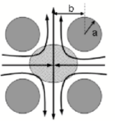
Figure 1: Schematic of the four-roll-mill flow profile. The geometry of the rollers, $a=6.6$ mm and $b=10.5$ mm, produces maximum homogeneity in the extension rate (Higdon, 1993; Fuller, 1997; Kooijman, 2000),. The shaded ellipse shows the area illuminated by the laser beam.

II Hydrodynamics

Our model (Alexander et al., 2007) describes the dynamics of a Langmuir layer consisting of two phases: an isolated phase-domain, $\Omega$, of finite area surrounded by a second Langmuir phase, $\Omega^{C}$, which extends infinitely in the horizontal direction. The Langmuir layer is modeled as a flat, two-dimensional fluid. We assume that the subfluid is infinitely deep. Both the Langmuir layer and the subfluid are assumed to be incompressible on the timescale of the relaxation experiments. Thus, the Langmuir domain $\Omega$ will have a fixed area, $A_{*}$.

For the Langmuir layer, the incompressibility condition in relaxation driven by line tension alone corresponds to a Gibbs elasticity $\kappa_{g}\gg\lambda/\sqrt{A_{*}}$, where $\lambda$ is the inter-phase line tension Alexander et al. (2006). For the experimentally accessible range we estimate that $\sqrt{A_{*}}>10\mu m$ and conservatively choose an upper limit on the line tension of $\lambda<1nN$, which yields an upper bound on the Gibbs elasticity, $\kappa_{g}\gg 10^{-4}N$, for significant compressibility. Thus, almost any Langmuir layer liquid and many gasses will act as incompressible fluids in line-tension driven relaxation processes (see Alexander et al. (2006) and references therein). In the special case of multilayers considered here, it is additionally conceivable that the number of layers might change during the relaxation process, leading to an area change. In practice, the thickness of the layers and the area of the domains were observed to be constant for the duration of the experiments reported here.

As we discuss above, dimensional analysis indicates that for 8CB the energy dissipated by viscous shearing within the Langmuir layer is much less than the amount dissipated by viscous shearing of the subfluid; we therefore model the Langmuir layer as inviscid. Furthermore, the subfluid can be treated in the Stokesian limit, where its inertia is negligible.

We non-dimensionalize the dynamics in terms of a characteristic length, time, and mass

$$L_{*}=\sqrt{A_{*}},\;\;T_{*}=\frac{\eta^{\prime}A_{*}}{\lambda},\;\;M_{*}=\eta^{\prime}L_{*}T_{*},$$ (1)

respectively; here $\lambda$ is the inter-phase line tension and $\eta^{\prime}$ is the subfluid viscosity. Essentially, the relaxation of the domain $\Omega$ is driven forward by the line tension between phases, and slowed by the viscosity of the subfluid.

The model ultimately yields an equation of motion for the boundary curve, $\vec{\Gamma}$, separating $\Omega$ and $\Omega^{C}$. As the boundary is isotropic, it suffices to determine the normal velocity, ${\cal U}$, to specify the domain’s evolution. We obtain (Alexander et al., 2007)

$${\cal U}=\left(\frac{\partial\Psi}{\partial s}\right)\hat{n}$$ (2)

where $\hat{n}$ is the outward unit normal vector to $\vec{\Gamma}$, $s$ is the arclength measured in a right-handed sense, and $\Psi(s)$ is the velocity streamfunction restricted to the boundary of the domain. This is computed as a boundary integral,

$$\Psi(s)=-\frac{1}{2\pi}\oint_{\vec{\Gamma}}\kappa(s^{\prime})\left[\hat{t}(s^{\prime})\cdot\hat{Q}(s,s^{\prime})\right]~{}ds^{\prime}\mbox{ ,}$$ (3)

where $\kappa$ is the curvature, $\hat{t}$ is the unit tangent vector, and $\hat{Q}(s,s^{\prime})$ is a unit vector pointing from $\vec{\Gamma}(s)$ to $\vec{\Gamma}(s^{\prime})$. A derivation and discussion of this formulation is given in (Alexander et al., 2007).

We implement a numerical solution in MATLAB. The problem is extremely stiff numerically; explicit integration methods are very susceptible to high-wavenumber instabilities. This can be ameliorated by operator splitting, following the ideas of Hou et al. (1994). While such a splitting in not immediately apparent in the formulation above, the formulation in Lubensky and Goldstein (1996) and Heinig et al. (2004) can be used to show that the high-frequency modes of $\vec{\Gamma}$ are asymptotically governed by a much simpler evolution law, namely motion by mean curvature.

As in (Hou et al., 1994), using an intrinsic description of the boundary allows an accurate implicit solution for the high-wavenumber modes, avoiding numerical instabilities. We represent the boundary with an equal-arclength discretization. Derivatives are computed pseudo-spectrally (Gottlieb and Orszag, 1977; Trefethen, 2000), and the boundary integral is computed using the 16-panel closed Newton-Cotes formula which guarantees high-order spatial accuracy. It is straightforward to solve the evolution by mean curvature implicitly and to high accuracy (Hou et al., 1994). We proceed by using Strang splitting (Strang, 1968) with the mean-curvature step implemented implicitly and the boundary integral velocity minus the mean curvature velocity computed explicitly.

Numerically, we observe a slow drift of the grid which forces us to regularly correct the arclength discretization — this is done using spectral interpolation and Newton-Raphson iteration. Also, it is necessary to filter the highest-frequency modes of $\vec{\Gamma}$ (whose numerical accuracy is poor due to the discretization anyway); we convolve the spectrum with a smooth filter and retain roughly two-thirds the spectrum. Details of the numerical implementation are available in (Pugh, 2006).

III Finding the Boundary Curves

To analyze a set of experimental photographs we must first determine the location of the boundary curve in each one. A grey-scale photograph is a map from each pixel $(x,y)$ to the brightness of the image at that location, $B(x,y)$. The edge of the domain is located in the region of rapid transition from black to white, where $||\nabla B||$ is large. We compute $\nabla B$ and $||\nabla B||$, using code developed by Fisher et al (Fischer et al., 2006). We execute a curve-tracing algorithm that “walks” around the edge of the domain, staying in the thin region where $||\nabla B||$ is large. As the algorithm traverses the boundary it marks points, which we subsequently use as a discrete representation of the boundary curve.

The placement of the edge can be quickly verified visually. We also have a quantitative check at our disposal. The domain area is conserved; if the edge is placed too far to the outside or inside then as the perimeter of the domain decreases during relaxation the computed area of the domain decreases or increases, respectively. This relationship allows us to calculate the (average) distance by which the edge is displaced in the normal direction. In most data sets we see no correlation between perimeter length and domain area. When this effect is seen, the implied displacement is never more than two pixels, and we can move the edge in the normal direction to correct for the displacement (this was done in data sets B and E reported below).

The greatest obstacle to determining the precise location of the edge is diffraction, which blurs the edge and produces a bright ring of constructive interference. Although the average normal displacement of the curve is very small, diffraction may cause the edge to be off by several pixels locally (this problem affects both human visual perception and computer algorithms).

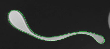
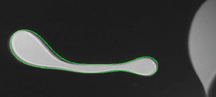
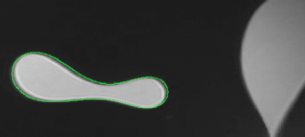
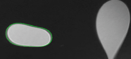
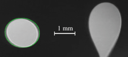
Figure 2: A series of snapshots (for data set B) showing the relaxation of a stretched domain to a circle. The snapshots are separated by 2.85 seconds $\approx$ 0.558 $T_{*}$. The first photo is superimposed with a curve marking the boundary determined by our edge-finding algorithm; this is the initial condition for the simulation of the domain relaxation. In subsequent photos the superimposed curve shows the simulated shape of the bola, based on that initial condition. The simulation accurately reproduces the observed dynamics even for complex, asymmetrical domains. The line tension of this domain is found to be $390\pm 3$ pN, where the uncertainty corresponds to the standard deviation of $T_{*}$. A movie of this relaxation is available from http://www.math.hmc.edu/~ajb/bola/simulation.mpeg.

IV Determining $\lambda$ via Experiment/Simulation Comparison

Our equation of motion (2) is written in time units of the characteristic relaxation time, defined by $T_{*}=\frac{\eta^{\prime}A_{*}}{\lambda}$. We calculate the line tension, $\lambda$, given these other values. The domain’s area, $A_{*}$, is determined from the photograph once the boundary curve is found, and the subfluid viscosity, $\eta^{\prime}$, is estimated from tabulated values (adjusting for temperature). We determine $T_{*}$ by simulating the evolution and matching timescales between the observed relaxation (snapshot times are recorded in seconds) and the simulated relaxation (done in units of $T_{*}$).

We choose an initial condition taken from one of the snapshots and simulate the subsequent relaxation. For each photograph after this first one, we match timescales by finding the time in the simulation when the shape of the simulated domain most closely matches the domain shape in the photo. We search through the discrete time-steps of the simulation and compare the shape at each step to the shape taken from the photo. Each snapshot gives us a value for $T_{*}$, computed as

$$T_{*}=\frac{t_{j}-t_{0}}{T_{best}-0}$$ (4)

where $t_{j}$ and $t_{0}$ are the observed times of the comparison snapshot and initial-condition snapshot, respectively, and $T_{best}$ is the time which elapses in the simulation between $T=0$ (the initial condition) and the time at which the best-matching shape occurs.

To measure how closely two domains (i.e. image-processed experiment and numerical simulation) match we use the Symmetric Difference Metric (SDM), which is determined by overlaying the domains and computing the total area which lies in one or the other but not both. For each photo, we search through the time-steps of the simulation to find the step at which the SDM between simulation domain and the experimental domain is minimized; Figure 3 provides a visual illustration of this process. The minimum SDM over the simulation provides a measure of how well each photo matches some shape which occurs in the simulation; we expect the same value for $T_{*}$ from every photo. We compute the mean value of the set of $T_{*}$’s from all the photos to determine the line tension, and the standard deviation of these $T_{*}$’s provides an estimate for the precision in the resulting measurement of $\lambda$.

To simulate the relaxation we must know the component of the subfluid velocity which exists independent of (i.e. is not directly produced by) the relaxation. Unfortunately, we cannot directly measure the subfluid velocity. Instead, we choose an initial snapshot when the subfluid is relatively quiescent and run the simulation under the approximation that the “independent” subfluid velocity is zero. We find, however, that the violation of this approximation is one of the largest sources of systematic error contributing to mismatch between observed and simulated domain shapes. We could choose a later initial condition, waiting until remnant subfluid velocity is negligible; however, this means throwing out a large portion of the data (often all of it).

The type of motion which persists in the subfluid for the longest time is solid-body motion; other types of motion are viscously damped. We therefore correct for solid-body motion in the post-simulation timescale fitting. Whenever we compare two shapes, we do not directly compute the SDM between them, but instead determine the minimum SDM which can be achieved by positioning one on top of the other using a solid-body motion. This greatly reduces the SDM and allows us to achieve excellent fits for data which would otherwise be rendered worthless by remnant subfluid velocity.

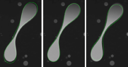
Figure 3: Three images showing the same photo overlayed with simulated boundary curves from three different times in the simulation. The center image shows the simulated curve at the time, $T_{best}$, when it most closely matches the photo; the left and right images show the simulated curve at $T=T_{best}-0.1T_{*}$ and $T=T_{best}+0.1T_{*}$, respectively.

Following (Mann et al., 1995), we also measure the line tension by measuring the relaxation of small elliptical deformations of the boundary in the near circular limit, which we refer to as $\lambda_{\epsilon}$. The snapshots of the domain boundary are image processed, and FFT techniques are used to extract the amplitude of the elliptical ($n=2$) deformation. We then fit the exponential relaxation rate of this mode in the small amplitude limit.

Data Set	${\lambda_{avg}}$ [pN]	$\sigma_{\lambda}/{\lambda_{avg}}$	Average SDM	$\sigma_{A}/A_{avg}$	$\lambda_{\epsilon}$ [pN]
A	538	3.4%	3.9%	1.0%	468
B	390	0.8%	2.9%	0.7%	375
C	357	1.7%	3.0%	0.3%	362
D	570	2.0%	1.5%	0.1%	606
E	479	4.0%	1.5%	1.0%	485
F	191	0.4%	3.4%	0.5%	217

Table 1: Line tension values and error estimates for six data sets. Here $\lambda_{avg}$ is the line tension values averaged over snapshots from large aspect ratio of bolas through the relaxation to nearly circular domains. The percentage error in this measurement is estimated by normalizing the standard deviation of these measurements by the average line tension, $\sigma_{\lambda}/{\lambda_{avg}}$. The average of the SDM (Symmetric Difference Metric) normalized by the domain area in these snapshots reflects how closely the numerical simulation reproduces the experimental results. The standard deviation of the domain area, $\sigma_{A}$ divided by the average area, $A_{avg}$, is a proxy for the error in the image processing of the boundary. Finally, $\lambda_{\epsilon}$ is the line tension estimated from small amplitude perturbations from the final circular domain shape.

Comparison data for six separate relaxations is presented in Table 1. In six time series of different domains, the mean SDM between the experimental and simulated domains was 1.5-4% of the domain’s area, indicating that the proposed hydrodynamical model of domain evolution reproduces the shapes quite well; this is clear from the comparison snapshots in the evolution in Figure 2. The areas of the domains were constant across the time series to 0.1-1%, well within the uncertainties of the measurement due to diffraction at the domain edges. By matching time scales between the experiment and simulation, each photo after the first yields a value for $T_{*}$ in seconds; we deduce $\lambda_{avg}$ from these values. The percentage deviation of the values for $T_{*}$ from a set of photos ranges from 0.4%-4%, which also provide an error estimate on the line tension.

The greatest variances in $T_{*}$ and the largest SDM values (i.e. shape mismatches) occurred in those data sets where either (1) other domains nearly touched the domain of interest or (2) remnant subfluid shearing was particularly problematic. Provided that reasonably isolated domains can be produced and the subfluid flow can be well-controlled, it is possible to determine the line tension to a precision of $\sim\!\!1\%$.

Finally, we note that the line tension estimates, $\lambda_{\epsilon}$, from small perturbations of the final circular shape are off by up to 13 % – this is comforting, in that it is consistent with our results and variations observed in previous work (Mann et al., 1995). It suggests that our new methodology is both accurate and precise.

V Conclusions

In this paper we have described a method for determining the line tension driving the evolution of Langmuir layers. We are able to verify that our hydrodynamic model is consistent with the experiments and to determine the line tension with errors as small as 1%, more than an order of magnitude better than previous efforts.

While we believe our measurement are accurate, it is striking that we have observed a wide variation in line tensions (191-570 pN) for the 8CB system. One factor that contributes significantly to this variation is the thickness of both the compact domain and its surroundings. Experiments reported elsewhere Zou et al. (2007), using the relaxation of small deformations generated with a different deformation technique, systematically explore the dependence on the thickness of a compact domain 1-15 bilayers thick (on top of an unpaired monolayer) in a trilayer background. These experiments lead to a line tension, reflecting the elastic energy of the dislocation at the domain boundary, proportional to the Burgers vector Zou et al. (2007). In the experiments reported here, we estimate, from the observed brightness of the domains, that the lighter compact domains range from 10-24 bilayers thick and that the darker surrounding region is either three or five layers thick. Because of light scattering from the four-roll mill in our study the thickness of the dark region, expected to contribute to the line tension Geminard et al. (1998), is particularly uncertain. Other possible factors influencing the line tension include contamination and splitting of the boundary into two dislocation lines for very thick films Geminard et al. (1998). Our expectation is that by quantifying this system and others more carefully we will be able to determine the dominant causes of line tension and generate reproducible results. This is a promising area for future investigation.

The present model assumes that bulk viscosity dominates the relaxation and that both slip between layers and electrostatic effects are negligible. These conditions must be evaluated on a case-to-case basis. However, the current method can determine the line tension with any technique exploiting domain hydrodynamic response, including relaxation after coalescence of two domains (Roberts et al., 1997) or after stretching a domain with lasers tweezers (Wurlitzer et al., 2000). It can also be generalized to more complex situations involving three-phase contacts.

The boundary integral formulation here can be extended to incorporate more general potential forces such as electrostatics (cf. (Lubensky and Goldstein, 1996; Heinig et al., 2004)) and as such we believe that we have developed a valuable tool for deducing and verifying the form of the intermolecular potential in systems that exhibit more complex morphology such as circle-to-dogbone transitions and labyrinth formation (DeKoker and McConnell, 1993; McConnell, 1991). This promises to be fertile ground for future research.

References

- Adamson and Gast (1998) A. W. Adamson and A. P. Gast, Physical Chemistry of Surfaces, 6th edition (John Wiley and Sons, New York, 1998).
- Stottrup et al. (2004) B. Stottrup, S. L. Veatch, and S. L. Keller, Biophysical Journal 86, 2942 (2004).
- Baumgart et al. (2003) T. Baumgart, S. T. Hess, and W. W. Webb, Nature 425, 821 (2003).
- Benvegnu and McConnell (1992) D. J. Benvegnu and H. M. McConnell, J. Phys. Chem. 96, 6820 (1992).
- Mann et al. (1995) E. K. Mann, S. Hénon, D. Langevin, J. Meunier, and L. Léger, Phys. Rev. E 51, 5708 (1995).
- Lauger et al. (1996) J. Lauger, C. R. Robertson, C. W. Frank, and G. G. Fuller, Langmuir 12, 5630 (1996).
- Stone and McConnell (1995) H. A. Stone and H. M. McConnell, Proc. R. Soc. London Ser. A-Math. Phys. Sci. 448, 97 (1995).
- Alexander et al. (2007) J. C. Alexander, A. J. Bernoff, E. K. Mann, J. A. Mann, Jr., J. R. Wintersmith, and L. Zou, J. Fluid Mech. 571, 191 (2007).
- de Mul and Mann Jr. (1994) M. N. G. de Mul and J. A. Mann Jr., Langmuir 10, 2311 (1994).
- de Mul and Mann Jr. (1998) M. N. G. de Mul and J. A. Mann Jr., Langmuir 14, 2455 (1998).
- DeKoker and McConnell (1993) R. DeKoker and H. M. McConnell, J. Phys. Chem. 97, 13419 (1993).
- McConnell (1991) H. M. McConnell, Annual Review Of Physical Chemistry 42, 171 (1991).
- Chen et al. (1991) S. M. Chen, T. C. Hsieh, and R. P. Pan, Physical Review A 43, 2848 (1991).
- Mukai et al. (1997) K. Mukai, N. Makino, H. Usui, and T. Amari, Progress In Organic Coatings 31 , 179 (1997).
- Hénon (1991) S. H. Hénon, S. Meunier, Rev. Sci. Instrum. 62, 936 (1991).
- Hönig and Möbius (1991) D. Hönig and D. Möbius, J. Phys. Chem. 95, 4590 (1991).
- Zou et al. (2004) L. Zou, J. Wang, V. J. Beleva, E. E. Kooijman, S. V. Primak, J. Risse, W. Weissflog, A. Jakli, and E. K. Mann, Langmuir 20, 2772 (2004).
- Higdon (1993) J. J. L. Higdon, Phys. Fluids A 5, 274 (1993).
- Fuller (1997) G. G. Fuller, Curr. Opin. Colloid Interface Sci. 2, 153 (1997).
- Kooijman (2000) E. E. Kooijman (2000), Master’s thesis, Dept. of Physics, Kent State University.
- Lagnado and Leal (1990) R. Lagnado and L. Leal, Experiments in Fluids 9, 25 (1990).
- Alexander et al. (2006) J. C. Alexander, A. J. Bernoff, E. K. Mann, J. A. Mann, and L. Zou, Physics of Fluids 18, 062103 (2006).
- Hou et al. (1994) T. Hou, J. Lowengrub, and M. Shelley, Journal of Computational Physics 114, 312 (1994).
- Lubensky and Goldstein (1996) D. K. Lubensky and R. E. Goldstein, Phys. Fluids 8, 843 (1996).
- Heinig et al. (2004) P. Heinig, L. E. Helseth, and T. M. Fischer, New Journal of Physics 6, 189 (2004).
- Gottlieb and Orszag (1977) D. Gottlieb and S. A. Orszag, Numerical analysis of spectral methods: theory and applications (SIAM, Philadelphia, 1977).
- Trefethen (2000) L. N. Trefethen, Spectral methods in MATLAB (SIAM, Philadelphia, 2000).
- Strang (1968) G. Strang, SIAM Numerical Analysis 5, 506 (1968).
- Pugh (2006) J. M. Pugh (2006), Senior Thesis, Department of Physics, Harvey Mudd College.
- Fischer et al. (2006) R. B. Fisher, S. Perkins, A. Walker, and E. Wolfart, “Canny edge detector” in Hypermedia Image Processing Reference (Wiley, Edinburgh, 2006), URL http://www.cee.hw.ac.uk/hipr/html/canny.html.
- Geminard et al. (1998) J. C. Geminard, C. Laroche, and P. Oswald, Physical Review E 58, 5923 (1998), part A.
- Zou et al. (2007) L. Zou, J. Wang, P. Basnet, and E. K. Mann, To appear in Phys. Rev. E (2007), See also arXiv:0705.0176v1.
- Roberts et al. (1997) M. J. Roberts, E. J. Teer, and R. S. Duran, Journal Of Physical Chemistry B 101, 699 (1997).
- Wurlitzer et al. (2000) S. Wurlitzer, P. Steffen, and T. M. Fischer, Journal Of Chemical Physics 112, 5915 (2000).