Von Neumann’s expanding model on random graphs

Abstract

Within the framework of Von Neumann’s expanding model, we study the maximum growth rate $\rho^{\star}$ achievable by an autocatalytic reaction network in which reactions involve a finite (fixed or fluctuating) number $D$ of reagents. $\rho^{\star}$ is calculated numerically using a variant of the Minover algorithm, and analytically via the cavity method for disordered systems. As the ratio between the number of reactions and that of reagents increases the system passes from a contracting ($\rho^{\star}<1$) to an expanding regime ($\rho^{\star}>1$). These results extend the scenario derived in the fully connected model ($D\to\infty$), with the important difference that, generically, larger growth rates are achievable in the expanding phase for finite $D$ and in more diluted networks. Moreover, the range of attainable values of $\rho^{\star}$ shrinks as the connectivity increases.

1 Introduction

Von Neumann’s expansion problem was initially formulated to describe growth in production economies as an autocatalytic process and has played a key role in the development of the theory of economic growth [1, 2, 3]. In a nutshell, it concerns the calculation of the maximum growth rate achievable by an autocatalytic system of $M$ reactants (labeled by Greek indices like $\mu,\nu,\dots$) interconnected by $N$ chemical reactions (labeled by Roman indices like $i,j,\ldots$) specified by a given stoichiometric matrix. The basic ingredients are however sufficiently simple to be applicable in different contexts ranging from economics to systems biology.

In order to state the optimization problem in mathematical terms (see however [4] for a more detailed description), it is convenient to separate the matrix of input stoichiometric coefficients $\boldsymbol{A}=\{a_{i}^{\mu}\geq 0\}$ (input matrix for brevity) from that of outputs $\boldsymbol{B}=\{b_{i}^{\mu}\geq 0\}$. The relevant microscopic variables are the reaction fluxes, denoted by $s_{i}$, which are assumed to be non-negative. The problem amounts to finding a vector $\boldsymbol{s}=\{s_{i}\geq 0\}$ of positive fluxes and a number $\rho>0$ such that $\rho$ is maximum subject to

$$\boldsymbol{B}\boldsymbol{s}\geq\rho\boldsymbol{A}\boldsymbol{s}$$ (1)

where the inequality is to be understood component-wise i.e. valid for each reactant $\mu$. The trivial null solution $\boldsymbol{s}=\boldsymbol{0}$, viz. $\{s_{i}=0~{}\forall i\}$, is not accepted: at least one component of $\boldsymbol{s}$ must be strictly positive.

Condition (1) requires that the total output of every reactant is at least $\rho$ times the total input. So the maximum feasible $\rho$, $\rho^{\star}$, measures the largest uniform growth rate achievable by the given set of reactions. If $\rho^{\star}<1$, the optimal state of the system is a contracting one. Otherwise for $\rho^{\star}>1$ it is expanding. The case $\rho^{\star}=1$ describes instead a system in which at optimality reaction fluxes are arranged so as to guarantee mass balance.

Von Neumann’s problem has been studied recently in a statistical mechanics perspective under the assumptions that $M$ scales linearly with $N$ (with $N\to\infty$) and that the stoichiometric matrices $\boldsymbol{A}$ and $\boldsymbol{B}$ have quenched random independent and identically distributed elements [4]. With a fully connected network of reactions (that is, one in which every reaction uses each reactant both as an input and as an output), one finds a transition from a contracting to an expanding regime when the parameter $n=N/M$ exceeds the critical value $n_{c}=1$.

In this work we extend the analysis of [4] to the finitely connected case where reactions use a finite number of inputs to produce a finite number of outputs. By analogy with integer programming problems (see e.g. [5]), we represent our autocatalytic network as a bipartite (factor) graph (see Fig. 1).

Figure 1: Factor graph representation of a network of reactions and reagents. Reactions are represented by circles, reagents by squares. Stoichiometric coefficients label the directed links.

We denote reagents as squares and reactions as circles. Each circle has a number of incoming (resp. outgoing) connections to squares, representing the inputs (resp. outputs) of the reaction, and each of these links carries the input (resp. output) stoichiometric coefficient. Similarly, each square has a number of incoming (resp. outgoing) connections to circles, denoting the reactions where that reagent enters as an output (resp. input). The notation $i\in\mu$ identifies a reaction $i$ in which a reactant $\mu$ is involved either as an input or as an output (and vice-versa for $\mu\in i$). To each reaction node a variable $s_{i}\geq 0$ is attached, representing the flux of reaction $i$. Each reactant node $\mu$ carries instead a function $c^{\mu}$ given by

$$c^{\mu}=\sum_{i\in\mu}s_{i}(b_{i}^{\mu}-\rho a_{i}^{\mu})$$ (2)

We are interested in finding non-null flux configurations satisfying (1), that is such that $c^{\mu}\geq 0$ for each $\mu$ and specifically in finding the largest value of $\rho$ for which a configuration of this type exists. Our approach is developed along two main lines. On the one hand (Section 2), we employ a suitably modified Minover algorithm to compute optimal growth rates numerically on any graph. Results thus derived will be theoretically validated in Section 3, where we use the cavity method to describe solutions analytically for locally tree-like instances. This approximation turns out to be in good qualitative agreement with numerical data. The connection of the latter approach with the fully connected theory developed in [4] is presented in two detailed Appendices.

2 Numerical analysis

2.1 Algorithm

Formula (1) is reminiscent of pattern storage conditions in the perceptron, a formal neural network model [6]. This analogy allowed us to devise an exact algorithm to solve Von Neumann’s problem on any graph in a time growing only polynomially with the number $N$ of nodes. The algorithm is an extension of the so-called Minover algorithm [7] enforcing the constraint of positivity for the fluxes, and hereafter referred to as Minover⁺.

The core part of the algorithm is a subroutine, Minover${}^{+}(\rho)$, we now describe. We assume that the matrices $\boldsymbol{A},\boldsymbol{B}$ are given, and $\rho$ denotes a real, non-negative number.

1. Step $\ell=0$: all fluxes are null, $s_{i}=0$.

2. Step $\ell+1$: Calculate the $M$ functions $c^{\mu}(\ell)$ defined in (2) from the values $s_{i}(\ell)$ of the fluxes at step $\ell$, and look for the reactant with least value,

   $$\mu_{0}(\ell)={\rm arg}~{}\min_{\mu}c^{\mu}(\ell)\ ;$$ (3)

   * if $c^{\mu_{0}(\ell)}\geq 0$ then OUTPUT $\boldsymbol{s}(\ell)$ and HALT (the null solution is not accepted);

   * otherwise, if $c^{\mu_{0}(\ell)}<0$, update the fluxes according to the rule

   $$s_{i}(\ell+1)=\max\{0,s_{i}(\ell)+b_{i}^{\mu_{0}(\ell)}-\rho\,a_{i}^{\mu_{0}(\ell)}\}\ ,$$ (4)

   increase $\ell$ by one, and GO TO (ii).

In case of ties, one may select $\mu_{0}$ at random uniformly among those with the same (and lowest) values of $c^{\mu}$.

We claim that, if $\rho<\rho^{\star}$, the largest growth rate associated to matrices $\boldsymbol{A}$ and $\boldsymbol{B}$, Minover${}^{+}(\rho)$ will halt after a finite number of steps, and output a set of non-negative fluxes guaranteeing a growth rate larger than $\rho$. The proof is simple and goes as follows. Assume $\rho<\rho^{\star}$. Then there exists a strictly positive number $\Delta$, hereafter called stability, and a vector $\boldsymbol{s}^{\star}\neq\boldsymbol{0}$ of fluxes such that

$$\boldsymbol{s}^{\star}\cdot(\boldsymbol{b}^{\mu}-\rho\boldsymbol{a}^{\mu})\geq\Delta\;|\boldsymbol{s}^{\star}|~{}~{}~{}~{}{\rm for~{}each~{}}\mu\ .$$ (5)

Let

$$A=\max_{\mu}\sum_{i}(b_{i}^{\mu}-\rho\,a_{i}^{\mu})^{2}>0\ .$$ (6)

and consider the functions $\mathcal{N}(\ell)=\boldsymbol{s}^{\star}\cdot\boldsymbol{s}(\ell)$ and $\mathcal{D}(\ell)=|\boldsymbol{s}(\ell)|^{2}$. We have, from (4),

$$\mathcal{N}(\ell+1) = \sum_{i}s_{i}^{\star}\;\max\{0,s_{i}(\ell)+b_{i}^{\mu_{0}(\ell)}-\rho\,a_{i}^{\mu_{0}(\ell)}\}$$

$$\geq \sum_{i}s_{i}^{\star}\;(s_{i}(\ell)+b_{i}^{\mu_{0}(\ell)}-\rho\,a_{i}^{\mu_{0}(\ell)})$$

$$\geq \mathcal{N}(\ell)+\Delta\;|\boldsymbol{s}^{\star}|$$

from the non-negativity of $s_{i}^{\star}$ and (5). We thus obtain $\mathcal{N}(\ell)\geq\ell\,\Delta\;|\boldsymbol{s}^{\star}|$ for any step $\ell$. Turning to function $\mathcal{D}(\ell)$ we get

$$\mathcal{D}(\ell+1) = \sum_{i}\max\{0,s_{i}(\ell)+b_{i}^{\mu_{0}(\ell)}-\rho\,a_{i}^{\mu_{0}(\ell)}\}^{2}$$

$$\leq \sum_{i}(s_{i}(\ell)+b_{i}^{\mu_{0}(\ell)}-\rho\,a_{i}^{\mu_{0}(\ell)})^{2}$$

$$= \mathcal{D}(\ell)+2\,c^{\mu_{0}(\ell)}+\sum_{i}(b_{i}^{\mu_{0}(\ell)}-\rho\,a_{i}^{\mu_{0}(\ell)})^{2}$$

$$\leq \mathcal{D}(\ell)+A$$

from definition (6) and the assumption that the algorithm has not halted at step $\ell$ i.e. $c^{\mu_{0}(\ell)}<0$. Hence $\mathcal{D}(\ell)\leq\ell\;A$. Now let

$$f(\ell)=\frac{\boldsymbol{s}(\ell)\cdot\boldsymbol{s}^{\star}}{|\boldsymbol{s}(\ell)|\;|\boldsymbol{s}^{\star}|}$$ (9)

By Cauchy-Schwarz inequality $f(\ell)\leq 1$. But according to the above calculations

$$f(\ell)=\frac{\mathcal{N}(\ell)}{|\boldsymbol{s}^{\star}|\sqrt{\mathcal{D}(\ell)}}\geq\frac{\Delta}{\sqrt{A}}\;\sqrt{\ell}\ .$$ (10)

Therefore the algorithm halts after

$$\ell_{0}=\frac{A}{\Delta^{2}}$$ (11)

steps at most. Now call $\ell_{s}$ the step at which the algorithm stops. The halting condition ensures that $c^{\mu_{0}(\ell_{s})}\geq 0$, i.e. condition (1) is satisfied, with a non-null vector of fluxes (by construction the fluxes are non-negative at any step). Hence $\boldsymbol{s}(\ell_{s})$ is a solution to Von Neumann’s problem with growth rate $\rho$.

Our complete algorithm, Minover⁺, is an iteration of Minover${}^{+}(\rho)$ for increasing values of $\rho$. Starting from $\rho=\epsilon$, a small positive value for which (1) surely admits a solution , one can measure the convergence time (number of steps prior to halting) $\ell_{s}$ for increasing values of $\rho$. The convergence time increases too. Now we expect $\Delta$ to vanish as $\rho^{\star}-\rho$ when $\rho$ gets closer and closer to its optimal value, thus $\ell_{s}\sim(\rho^{\star}-\rho)^{-2}$ from (11) (see Fig. 2).

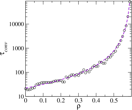
Figure 2: Convergence time (in individual steps) versus $\rho$ for a single network with $M=100$ reagents and $n=0.66$. The number of reagents per reaction is fixed at $D=5$, the number of reactions per reagent is a Poisson random variable with mean $Dn=3.3$. The dashed line represents the best fit with $\tau_{conv}\sim(\rho^{\star}-\rho)^{-2}$. For this network, $\rho^{\star}=0.5994$.

One may then estimate the maximal growth rate by extrapolating from the log-log plot of the convergence time versus $\rho$.

2.2 Survey of results

In what follows we restrict ourselves to purely autocatalytic systems, that is we assume that every reagent is produced and consumed by at least one reaction. Indeed a reagent that only serves as input gives rise to a constraint of the form

$$c^{\mu}=-\rho\sum_{i\in\mu}s_{i}a_{i}^{\mu}\geq 0$$ (12)

which is satisfied by taking $\rho=0$. Such a situation would immediately force the result $\rho^{\star}=0$. On the other hand, “sink” reagents (namely those that are not inputs of any reaction) provide constraints that are $\rho$-independent and trivially satisfied. Furthermore, for the sake of simplicity, we fix the number $M$ of reagents and assume that the quenched random stoichiometric matrix has Gaussian elements with mean $1$ and variance $1/2$.

For a start, we consider Von Neumann’s problem on factor graphs in which every reaction has $D$ inputs and $D$ outputs, while for reagents we assume that the in(out)-degree distribution is Poissonian, $P(k)=\lambda^{k}e^{-\lambda}/k!$ with mean degree $\lambda=Dn$. For short, we write Regular$(N)$/Poisson$(M)$ to denote this type of situation. Our analysis focuses on values of $n=N/M>1/D$, which ensure that the resulting factor graph is connected. Results for $\rho^{\star}$ in this case are displayed in the left panel of Fig. 3.

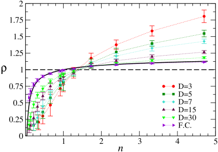
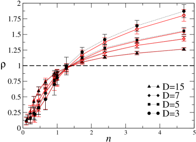
Figure 3: Left panel: $\rho^{\star}$ vs $n$ for Regular$(N)$/Poisson$(M)$ networks of 100 reagents for various $D$. The continuous line is the fully-connected limit for a system of the same size [4] while F.C. labels numerical results for a fully connected system. Right panel: $\rho^{\star}$ vs $n$ for Regular$(N)$/Poisson$(M)$ (open markers) and Regular$(N)$/SF$(M)$ (closed markers) networks for different values of $D$ (see text for details). Averages over 50 samples.

One sees that the overall qualitative behaviour reproduces the results obtained for the fully connected model. The system passes from an expanding ($\rho^{\star}>1$) to a contracting ($\rho^{\star}<1$) phase when $n$ is lowered below a critical value. Interestingly, the maximum growth rate achievable in the diluted system is larger than in the fully connected model in the expanding phase and higher growth rates can be achieved in more diluted systems. This conclusion turns out to be valid generically for all types of networks we studied.

In the right panel of Fig. 3 we compare these results with those obtained for the case in which the number of reactions per reagent is power-law distributed (SF or scale-free for short) rather than Poisson, which enables the coexistence of widely used and rarely used reagents in the reaction network (reactions still have a $\delta$-distributed connectivity). More precisely, the number of reactions per reagent is distributed as $P(k)\sim k^{-\gamma}$ with $2<\gamma<3$ (as in e.g. metabolic networks [9]). The particular value of the exponent does not affect results in a marked way. Note that a significant difference (which however lies inside the error bar) is observed only for the smallest values of $D$.

Next we compare networks with degree regular reactions, where, as said above, the in/out-degree of reactions is fixed equal to $D$, with Poisson$(N)$/Poisson$(M)$ networks where also reactions have fluctuating degree with mean $D$.

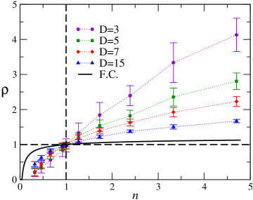
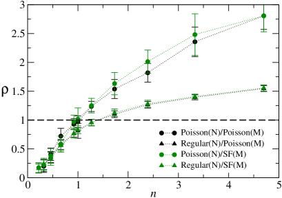
Figure 4: Left panel: $\rho^{\star}$ vs $n$ for Poisson$(N)$/Poisson$(M)$ networks. Right panel: $\rho^{\star}$ vs $n$ for different types of factor graphs with $D=5$. Averages over 50 samples; system of 100 reagents.

From Fig. 4 one sees that optimal growth rates for all values of $n$ are always larger in Poissonian networks than in regular ones, independently of the degree distribution of reagents (right panel). Moreover a fluctuating connectivity for reactions makes the expanding regime achievable with fewer reactions (left panel), and in particular the critical point where $\rho^{\star}$ becomes larger than 1 is $n_{c}\simeq 1$, similar to what is found in the fully connected case. In few words, we can say that topological regularity has a strong influence on the maximum growth rate achievable and that an asymmetric choice of degree distributions for reactions and reagents moves $n_{c}$ from its fully connected value. In the case above, it takes a larger repertoire of reactions to sustain an expanding regime.

It is possible to find a simple expression that allows to re-scale the data obtained for different $D$’s onto a single curve (which appears to be topology-dependent), at least for large $n$. It turns out that

$$\rho^{\star}(n,D)\simeq\rho^{\star}_{{\rm F.C.}}(n)+\frac{1}{D}f(n)$$ (13)

where $\rho^{\star}_{{\rm F.C.}}(n)$ is the optimal growth rate of the fully connected system (see Fig. 5).

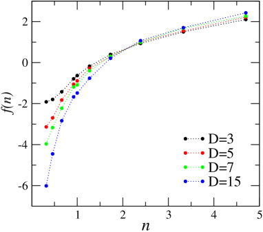
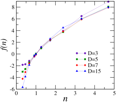
Figure 5: Scaling functions $f(n)$ for Regular$(N)$/Poisson$(M)$ networks (left) and Poisson$(N)$/Poisson$(M)$ networks (right). Error bars not reported.

This scaling form, which gives $\rho^{\star}$’s for diluted systems as $1/D$ corrections to the fully connected limit, implies that the range of achievable growth rates shrinks as $D$ increases.

In Fig. 6, we show the values of $\rho^{\star}$ for systems of different sizes and topologies (similar results hold for other types of networks).

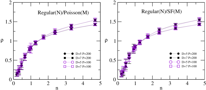
Figure 6: $\rho^{\star}$ vs $n$ for Regular$(N)$/Poisson$(M)$ and Regular($N$)/SF($M$) networks of 100 and 200 reagents for different $D$. Averages over 50 samples.

One sees that already for moderate system sizes finite size effect are negligible.

To conclude, we present (see Figures 7 and 8) the flux distribution at optimality for Regular$(N)$/Poisson$(M)$ and Poisson$(N)$/Poisson$(M)$ networks for values of $n$ below and above the critical point.

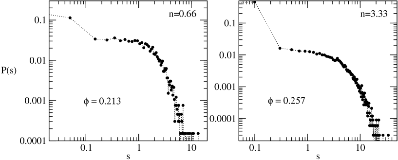
Figure 7: Flux distribution for a Regular$(N)$/Poisson$(M)$ network of reagents with $D=5$ inputs and outputs per reaction and different values of $n$ (average over 50 samples). System of 200 reagents. The $\delta$-peak at $s=0$ (carrying an intensive weight $\phi$ reported inside the panels) is not shown.

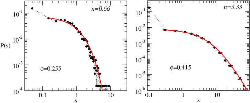
Figure 8: Flux distribution for a Poisson$(N)$/Poisson$(M)$ network of reagents with $D=5$ inputs and outputs per reaction and different values of $n$ (average over 50 samples). System of 200 reagents. The $\delta$-peak at $s=0$ (carrying an intensive weight $\phi$ reported inside the panels) is not shown. The red lines represent best fits with an exponential distribution of the form $p(x)=Ae^{-Bx}$ (left panel) and with an algebraic distribution of the form $p(x)=A(B+x)^{-C}$ (right panel).

In the former case, distributions are well fitted by an exponential form both for small and large $n$. In the latter case, an algebraic law provides the best fit in the expanding regime. Similar results are obtained for different connectivity distributions for reaction nodes. The particular value of the exponent appears to be topology dependent. However, it is interesting that such distributions arise in this context, specifically for their relevance in connection to metabolic networks [8, 9]. Note finally that as in the fully-connected model the weight of the mass at $s=0$ increases with $n$, though less drastically.

3 Cavity theory

Von Neumann’s problem possesses the natural cost function

$$E=\sum_{\mu=1}^{M}\Theta(-c^{\mu}),$$ (14)

that, given $\rho$, counts the number of reagents for which the condition (1) is violated. It is clear that $\rho^{\star}$ corresponds to the largest $\rho$ for which one can arrange fluxes in such a way that $E=0$. More generally, we can look for configurations that minimize $E$, so it is convenient to introduce the “partition function”

$$Z=\int\gamma(\boldsymbol{s})e^{-\beta E}d\boldsymbol{s}\equiv\Tr_{\boldsymbol{s}}e^{-\beta E}$$ (15)

with $\gamma(\boldsymbol{s})$ some constraint over the configuration space (e.g. a linear constraint). Minima of the cost function are selected in the limit $\beta\to\infty$.

Let us assume that the factor graph has a locally tree-like structure

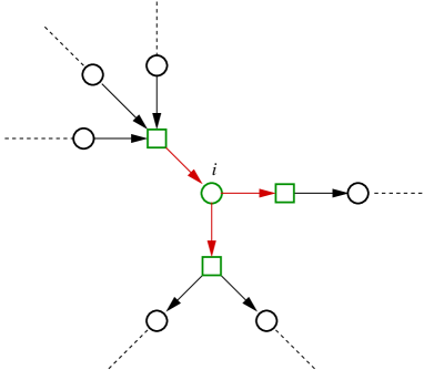
Figure 9: Left: reagents participating in reaction $i$ are correlated. Right: If reaction $i$ is removed those reagents become uncorrelated on a tree-like graph.

and consider, as in Figure 9, a reaction $i$ and the reagents involved in it. It is clear that the joint distribution of consumptions $\boldsymbol{c}^{\mu\in i}=\{c^{\mu}\}_{\mu\in i}$ does not factorize into single-reagent terms, i.e.

$$q(\boldsymbol{c}^{\mu\in i})\neq\prod_{\mu\in i}q^{\mu}(c^{\mu})$$ (16)

because the $\mu$’s share the common vertex $i$. However, if we remove the reaction $i$ (here and in what follows indexes enclosed in parentheses like $(x)$ denote quantities calculated removing the node $x$, while sums and products where $x$ is not considered carry the index $\backslash x$) the resulting joint distribution of consumptions $q_{(i)}(\boldsymbol{c}^{\mu\in i})$ does factorize:

$$q_{(i)}(\boldsymbol{c}^{\mu\in i})=\prod_{\mu\in i}q_{(i)}^{\mu}(c^{\mu})$$ (17)

Similarly, with $\boldsymbol{s}_{i\in\mu}=\{s_{i}\}_{i\in\mu}$, we have

$$p(\boldsymbol{s}_{i\in\mu})\neq\prod_{i\in\mu}p_{i}(s_{i})$$ (18)

but, removing reagent $\mu$,

$$p^{(\mu)}(\boldsymbol{s}_{i\in\mu})=\prod_{i\in\mu}p_{i}^{(\mu)}(s_{i})$$ (19)

The quantities $q_{(i)}^{\mu}(c^{\mu})$ and $p_{i}^{(\mu)}(s_{i})$ are known as cavity distributions. Now for all $i=1,\ldots,N$ and $\mu\in i$ it is possible to find equations for the cavity distributions by simply merging back all disconnected nodes but one (see Fig. 10). It is easily seen in particular that

$$p_{i}^{(\mu)}(s_{i}) = \frac{1}{Z_{i}^{(\mu)}}\int e^{-\beta\sum_{\nu\in i\backslash\mu}\Theta\left[-c_{(i)}^{\nu}-s_{i}(b_{i}^{\nu}-\rho a_{i}^{\nu})\right]}\prod_{\nu\in i\backslash\mu}q_{(i)}^{\nu}(c^{\nu})dc^{\nu}$$ (20)

$$\equiv \frac{1}{Z_{i}^{(\mu)}}\Tr_{\boldsymbol{c}^{\nu\in i\backslash\mu}}\left[\prod_{\nu\in i\backslash\mu}q_{(i)}^{\nu}(c^{\nu})\right]e^{-\beta\sum_{\nu\in i\backslash\mu}\Theta\left[-c_{(i)}^{\nu}-s_{i}(b_{i}^{\nu}-\rho a_{i}^{\nu})\right]}$$

(where $Z_{i}^{(\mu)}$ is a normalization factor ensuring that $\int p_{i}^{(\mu)}(s_{i})ds_{i}=1$) while for each $\mu=1,\ldots,M$ and $i\in\mu$ we have

$$q_{(i)}^{\mu}(c^{\mu})=\Tr_{\boldsymbol{s}_{j\in\mu\backslash i}}\left[\prod_{j\in\mu\backslash i}p_{j}^{(\mu)}(s_{j})\right]\delta\left[c^{\mu}-\sum_{j\in\mu\backslash i}s_{j}(b_{j}^{\mu}-\rho a_{j}^{\mu})\right]$$ (21)

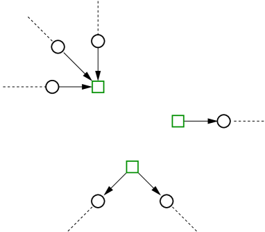
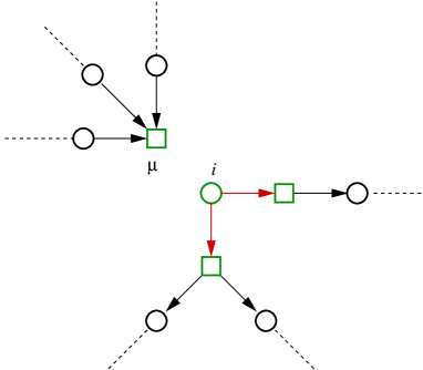
Figure 10: From the graph where reaction $i$ has been removed (left), one calculates easily the distribution $p_{i}^{(\mu)}(s_{i})$ in the absence of the reagent $\mu$ by merging back all reagents participating in reaction $i$ but reagent $\mu$.

Note that these in turn imply that

$$p_{i}(s_{i})=\frac{1}{Z_{i}}\Tr_{\boldsymbol{c}^{\nu\in i}}q_{(i)}(\boldsymbol{c}^{\nu\in i})e^{-\beta\sum_{\nu\in i}\Theta\left[-c_{(i)}^{\nu}-s_{i}(b_{i}^{\nu}-\rho a_{i}^{\nu})\right]}$$ (22)

$$q^{\mu}(c^{\mu})=\Tr_{\boldsymbol{s}_{j\in\mu}}p^{(\mu)}(\boldsymbol{s}_{j\in\mu})\delta\left[c^{\mu}-\sum_{j\in\mu}s_{j}(b_{j}^{\mu}-\rho a_{j}^{\mu})\right]$$ (23)

so that the whole probability distribution can be reconstructed from the set of cavity distributions. The statistical average cost function is finally given by

$$\left\langle{\frac{E}{N}}\right\rangle = \frac{1}{N}\sum_{\mu=1}^{M}{\rm Tr}_{c}\Theta(-c)\frac{q^{\mu}(c)\left[e^{-\beta}+(1-e^{-\beta})\Theta\left(c\right)\right]}{{\rm Tr}_{c}q^{\mu}(c)\left[e^{-\beta}+(1-e^{-\beta})\Theta\left(c\right)\right]}$$ (24)

The cavity theory developed here recovers the replica theory of [4] in the fully-connected limit. This is shown in detail in Appendices A, where a slightly revised replica theory is discussed, and B, where the fully connected limit is constructed explicitly.

Because the configurational variables $s_{i}$ and $c^{\mu}$ are continuous, solving equations (20) and (21), which in the zero temperature ($\beta\to\infty$) limit take the form

$$p_{i}^{(\mu)}(s_{i}) = \frac{1}{Z_{i}^{(\mu)}}\Tr_{\boldsymbol{c}^{\nu\in i\backslash\mu}}\left[\prod_{\nu\in i\backslash\mu}q_{(i)}^{\nu}(c^{\nu})\right]\prod_{\nu\in i\backslash\mu}\Theta\left[c_{(i)}^{\nu}+s_{i}(b_{i}^{\nu}-\rho a_{i}^{\nu})\right]$$ (25)

$$q_{(i)}^{\mu}(c^{\mu}) = \Tr_{\boldsymbol{s}_{j\in\mu\backslash i}}\left[\prod_{j\in\mu\backslash i}p_{j}^{(\mu)}(s_{j})\right]\delta\left[c^{\mu}-\sum_{j\in\mu\backslash i}s_{j}(b_{j}^{\mu}-\rho a_{j}^{\mu})\right],$$ (26)

by the standard method of population dynamics requires studying a population of populations, as e.g. in [10] (in other words, it is equivalent to a one-step RSB calculation already at the replica-symmetric level). We therefore decided to focus our analysis on the calculation of the optimal growth rate, for which it is possible to obtain good results at a modest computational cost.

We are thus interested in finding the critical line $\rho^{\star}(n)$. One may proceed as follows. Assume there is no linear constraint (the value of $\rho^{\star}$ is unaffected by the presence of a linear constraint). Then the equations always admit the trivial solution ($\boldsymbol{s}=\boldsymbol{0}$) for all values of $\rho$. In fact, for $\rho>\rho^{\star}$ this is the only zero-energy solution while below $\rho^{\star}$ other non-null solutions exist. Thus, starting from random initial conditions for the fluxes, we would expect the average flux to vanish (resp. remain different from zero) under the iteration of the cavity equations for values of $\rho$ above (resp. below) $\rho^{\star}$. This obviously assumes that the iteration of the cavity equations for $\rho<\rho^{\star}$ keeps the fluxes away from their trivial value, which turns out to be the case.

To check the validity of this assumption, we have first considered the cavity equations (25) and (26) in their fully connected limit (see Appendices for details), viz.

$$x_{(i)}^{\mu} = M_{0}\left(h^{\mu}_{(i)},\phi^{\mu}_{(i)}\right)$$ (27)

$$y_{(i)}^{\mu} = M_{1}\left(h^{\mu}_{(i)},\phi^{\mu}_{(i)}\right)$$ (28)

$$m_{\ell}^{(\mu)} = f_{1}\left(A^{(\mu)}_{\ell},B^{(\mu)}_{\ell}\right)$$ (29)

$$L_{\ell}^{(\mu)} = f_{2}\left(A^{(\mu)}_{\ell},B^{(\mu)}_{\ell}\right)$$ (30)

with

$$h^{\mu}_{(i)} = \frac{1}{\sqrt{K}}\sum_{\ell\in\mu\backslash i}\xi_{\ell}^{\mu}(\rho)m_{\ell}^{(\mu)}$$ (31)

$$\phi^{\mu}_{(i)} = \frac{1}{K}\sum_{\ell\in\mu\backslash i}[\xi_{\ell}^{\mu}(\rho)]^{2}[L_{\ell}^{(\mu)}-[m_{\ell}^{(\mu)}]^{2}]$$ (32)

$$A^{(\mu)}_{i} = \frac{1}{\sqrt{K}}\,\sum_{\nu\in i\backslash\mu}\xi_{i}^{\nu}(\rho)x_{(i)}^{\mu}$$ (33)

$$B^{(\mu)}_{i} = \frac{1}{2K}\sum_{\nu\in i\backslash\mu}[\xi_{i}^{\nu}(\rho)]^{2}\left(y_{(i)}^{\nu}+[x_{(i)}^{\nu}]^{2}\right)$$ (34)

$$\xi_{i}^{\mu}(\rho) = b_{i}^{\mu}-\rho a_{i}^{\mu}$$ (35)

and where $M_{s}(a,b)$ and $f_{k}(a,b)$ are defined as follows ($H(x)={\rm erfc}(x/\sqrt{2})/2$)

$$M_{s}(a,b) = \frac{\left(1-e^{-\beta}\right)\left(\frac{\partial}{\partial c}\right)^{s}\mathcal{G}_{c}(a,b)\Big{|}_{s=0}}{e^{-\beta}+(1-e^{-\beta})H\left(\frac{-a}{\sqrt{b}}\right)}~{}~{},~{}~{}~{}~{}~{}(\beta\to\infty)$$ (36)

$$f_{k}(a,b) = \frac{{\rm Tr}_{s}e^{as-bs^{2}}s^{k}}{{\rm Tr}_{s}e^{as-bs^{2}}}$$ (37)

with $\mathcal{G}_{c}(a,b)$ a Gaussian distribution for the variable $c$ with mean $a$ and variance $b$. For computational reasons, it is more convenient to iterate the corresponding TAP equations [11], namely

$$x^{\mu} = M_{0}\left(\frac{1}{\sqrt{K}}\sum_{\ell\in\mu}\xi_{\ell}^{\mu}(\rho)m_{\ell}-x^{\mu}\phi^{\mu},\phi^{\mu}\right)$$ (38)

$$y^{\mu} = M_{1}\left(\frac{1}{\sqrt{K}}\sum_{\ell\in\mu}\xi_{\ell}^{\mu}(\rho)m_{\ell}-x^{\mu}\phi^{\mu},\phi^{\mu}\right)$$ (39)

$$m_{i} = f_{1}\left(\frac{1}{\sqrt{K}}\,\sum_{\nu\in i}\xi_{i}^{\nu}(\rho)x^{\mu}+m_{i}B_{i},B_{i}\right)$$ (40)

$$L_{i} = f_{2}\left(\frac{1}{\sqrt{K}}\,\sum_{\nu\in i}\xi_{i}^{\nu}(\rho)x^{\mu}+m_{i}B_{i},B_{i}\right)$$ (41)

$$B_{i} = \frac{1}{2K}\sum_{\nu\in i}[\xi_{i}^{\nu}(\rho)]^{2}\left(y^{\nu}+(x^{\nu})^{2}\right)$$ (42)

$$\phi^{\mu} = \frac{1}{K}\sum_{i\in\mu}[\xi_{i}^{\mu}(\rho)]^{2}\left(L_{i}-m_{i}^{2}\right)$$ (43)

Given a matrix $\xi_{i}^{\mu}(\rho)$, we solve the preceding set of coupled equations by iteration: starting from a small value of $\rho$ we monitor the average flux and determine $\rho^{\star}$ when, under iteration of the equations, the average flux goes to zero. In Fig. 11 we compare the results for a system of $M=100$ reagents (average over 10 samples) with the theoretical prediction. The agreement is fairly good.

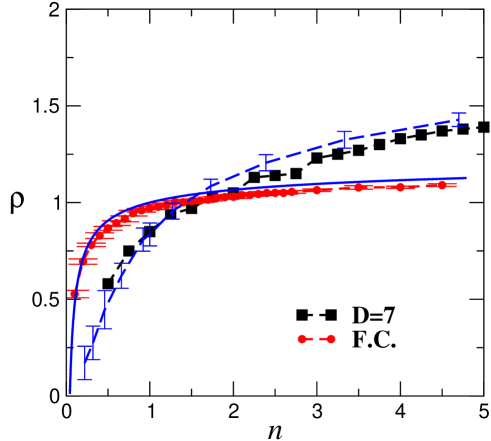
Figure 11: Results from cavity theory. The continuous (blue) line is the theoretical (replica) prediction in the fully connected limit. The dashed line represents Minover results for Regular($N$)/Poisson ($M$) graphs, with error bars. Markers correspond to iteration of the fully connected (circles, average over 10 samples, number of reagents $M=100$) and Regular($N$)/Poisson ($M$) cavity equations (squares).

We have then considered the same approach to calculate $\rho^{\star}$ for a Regular$(N)$/Poisson$(M)$ network with connectivity $D=7$ (see Fig. 11). To do so, we have considered the ensemble version of equations (25) and (26), which take the form (we suppress cavity indexes $(x)$ for simplicity)

$$p_{i}(s) = \frac{1}{Z_{i}}\prod_{\nu=1}^{2D-1}\Bigg{[}\Tr_{{c}^{\nu}}q^{\nu}(c^{\nu})\Theta\left[c^{\nu}+s(b_{i}^{\nu}-\rho a_{i}^{\nu})\right]\Big{]}$$ (44)

$$q^{\mu}(c) = \left[\prod_{j=1}^{k_{\mu}-1}\Tr_{{s}_{j}}p_{j}(s_{j})\right]\delta\left[c-\sum_{j=1}^{k_{\mu}-1}s_{j}(b_{j}^{\mu}-\rho a_{j}^{\mu})\right]$$ (45)

with $k_{\mu}$ a random Poisson number with average $nD$. In the ensemble, which is obtained after the limit $N\to\infty$ has been performed and where $n$ plays the role of an external parameter, the indexes $i$ and $\mu$ now take values $i,\mu=1,2,3,\ldots$ and describe an infinite population of probabilities $\{q^{\mu}(c)\}_{\mu=1,2,\ldots}$ and $\{p_{i}(s)\}_{i=1,2,\ldots}$. We have studied a finite population of probabilities, i.e. $i,\mu=1,\ldots,\mathcal{N}_{pop}$, which are initialised randomly. In order to find $\rho^{\star}$, we start from a small initial value for $\rho$. The population is iterated via equations (44) and (45). If after a certain (sufficiently large) number of iteration steps the average flux is different from zero, we increase the value of $\rho$ by a small value and restart the procedure. Eventually we can locate a value of $\rho$ at which the average flux vanishes. This defines $\rho^{\star}$. In Fig. 11 we display the resulting curve $\rho^{\star}(n)$ for a population of $\mathcal{N}_{pop}=50$ distributions and $D=7$, which qualitatively agrees with the results found by the Minover⁺ algorithm. (We remind that cavity equations are obtained for a tree-like topology and the network we considered in the numerical solution is relatively small.)

4 Summary

Despite evident quantitative differences, the overall picture obtained for the fully-connected Von Neumann’s model is roughly preserved in the case of finite connectivity, discussed here. The major difference appears to be that much larger growth rates can be achieved in diluted networks (reactions with few inputs/outputs are evidently more efficient) and, generically, when reactions have stochastic connectivities. The framework of Von Neumann’s problem, including its global optimization aspect, is sufficiently simple to ensure that the methods developed in this work can be applied in several different contexts, particularly in economics and biology. Work along both lines is in progress.

References

Appendix A The fully-connected model revisited

We shall briefly re-consider here the replica approach of [4] for the fully connected model in the Derrida-Gardner framework (as opposed to the Gardner one employed in [4]). This allows us to derive equations for the order parameters that are easily compared with those which shall be derived in the following section as the fully connected limit of the cavity theory.

Our starting point is the partition function, which we write in this case

$$Z=\Tr_{\boldsymbol{c}}\prod_{\mu=1}^{M}\left[e^{-\beta}+(1-e^{-\beta})\Theta(c^{\mu})\right]\Tr_{\boldsymbol{s}}\prod_{\mu=1}^{M}\delta\left(c^{\mu}-\frac{1}{\sqrt{N}}\sum_{i=1}^{N}s_{i}\xi_{i}^{\mu}(\rho)\right)$$ (46)

where

$$\xi_{i}^{\mu}(\rho)=b_{i}^{\mu}-\rho a_{i}^{\mu}$$ (47)

As in [4], we write $b_{i}^{\mu}=\overline{b}(1+\beta_{i}^{\mu})$ and $a_{i}^{\mu}=\overline{a}(1+\alpha_{i}^{\mu})$ with Gaussian $\alpha_{i}^{\mu}$ and $\beta_{i}^{\mu}$ and further set $\overline{a}=\overline{b}=1$. Moreover, we re-cast $\rho$ as $\rho=1+g/\sqrt{N}$ so that

$$\xi_{i}^{\mu}(\rho)=\beta_{i}^{\mu}-\alpha_{i}^{\mu}-\frac{g}{\sqrt{N}}(1+\alpha_{i}^{\mu})$$ (48)

The replicated and disorder-averaged partition function reads

$$\overline{Z^{r}}=\Tr_{\{\boldsymbol{c}_{1},\ldots,\boldsymbol{c}_{r}\}}\prod_{\ell=1}^{r}\prod_{\mu=1}^{M}\left[e^{-\beta}+(1-e^{-\beta})\Theta(c^{\mu}_{\ell})\right]$$

$$\hskip 28.45274pt\times\Tr_{\{\boldsymbol{s}_{1},\ldots,\boldsymbol{s}_{r}\}}\overline{\prod_{\ell=1}^{r}\prod_{\mu=1}^{M}\delta\left(c_{\ell}^{\mu}-\frac{1}{\sqrt{N}}\sum_{i=1}^{N}s_{i\ell}\xi_{i}^{\mu}(\rho)\right)}$$ (49)

If the $\delta$-distributions are written in their Fourier representation (with multipliers $\widehat{c}_{\ell}^{\mu}$) the disorder average can be carried out easily, generating the standard order parameters

$$q_{\ell\ell^{\prime}}=\frac{1}{N}\sum_{i}s_{i\ell}s_{i\ell^{\prime}}~{}~{}~{}~{}~{}~{}~{}m_{\ell}=\frac{1}{N}\sum_{i}s_{i\ell}$$ (50)

which can be forced into the partition function with proper Lagrange multipliers $\widehat{q}_{\ell\ell^{\prime}}$ and $\widehat{m}_{\ell}$. One finally finds

$$\overline{Z^{r}}=\int D\boldsymbol{q}D\widehat{\boldsymbol{q}}D\boldsymbol{m}D\widehat{\boldsymbol{m}}~{}e^{N[\sum_{\ell\leq\ell^{\prime}}\widehat{q}_{\ell\ell^{\prime}}q_{\ell\ell}+\sum_{\ell}\widehat{m}_{\ell}m_{\ell}+F(\boldsymbol{q},\boldsymbol{m})+S(\widehat{\boldsymbol{q}},\widehat{\boldsymbol{m}})]}$$ (51)

where ($\alpha=M/N,\kappa\equiv\overline{(\beta_{i}^{\mu}-\alpha_{i}^{\mu})^{2}}$)

$$F(\boldsymbol{q},\boldsymbol{m})=\alpha\log\int\left[\prod_{\ell=1}^{r}\frac{dc_{\ell}d\widehat{c}_{\ell}}{2\pi}\right]e^{i\sum_{\ell=1}^{r}\widehat{c}_{\ell}c_{\ell}+{\rm i}g\sum_{\ell=1}^{r}\widehat{c}_{\ell}m_{\ell}-\frac{\kappa}{2}\sum_{\ell,\ell^{\prime}}\widehat{c}_{\ell}\widehat{c}_{\ell^{\prime}}q_{\ell\ell^{\prime}}}$$

$$\hskip 56.9055pt\times\prod_{\ell=1}^{r}\left[e^{-\beta}+(1-e^{-\beta})\Theta(c_{\ell})\right]$$

$$S(\widehat{\boldsymbol{q}},\widehat{\boldsymbol{m}})=\frac{1}{N}\log\Tr_{\{\boldsymbol{s}_{\ell}\}}\,e^{-\sum_{\ell\leq\ell^{\prime}}\widehat{q}_{\ell\ell^{\prime}}\sum_{i=1}^{N}s_{i\ell}s_{i\ell^{\prime}}-\sum_{\ell}\widehat{m}_{\ell}\sum_{i=1}^{N}s_{i\ell}}$$

In the limit $N\to\infty$, the integral (51) is evaluated by a saddle-point method. Let us consider the saddle-point equation for the order parameter $\widehat{q}_{\ell\ell^{\prime}}$ ($\ell\neq\ell^{\prime}$):

$$\widehat{q}_{\ell\ell^{\prime}}=\kappa\alpha\frac{\int\prod_{\ell}\frac{dc_{\ell}d\widehat{c}_{\ell}}{2\pi}~{}\widehat{c}_{\ell}\widehat{c}_{\ell^{\prime}}~{}e^{i\sum_{\ell=1}^{r}\widehat{c}_{\ell}c_{\ell}+{\rm i}g\sum_{\ell}\widehat{c}_{\ell}m_{\ell}-\frac{\kappa}{2}\sum_{\ell,\ell^{\prime}}\widehat{c}_{\ell}\widehat{c}_{\ell^{\prime}}q_{\ell\ell^{\prime}}}\prod_{\ell=1}^{r}\left[e^{-\beta}+(1-e^{-\beta})\Theta(c_{\ell})\right]}{\int\prod_{\ell}\frac{dc_{\ell}d\widehat{c}_{\ell}}{2\pi}~{}e^{i\sum_{\ell=1}^{r}\widehat{c}_{\ell}c_{\ell}+{\rm i}g\sum_{\ell}\widehat{c}_{\ell}m_{\ell}-\frac{\kappa}{2}\sum_{\ell,\ell^{\prime}}\widehat{c}_{\ell}\widehat{c}_{\ell^{\prime}}q_{\ell\ell^{\prime}}}\prod_{\ell=1}^{r}\left[e^{-\beta}+(1-e^{-\beta})\Theta(c_{\ell})\right]}$$ (52)

The argument of the exponential in the denominator can be linearized by a Hubbard-Stratonovich transformation. Once this is done, it is clear that the remaining integrals over $c_{\ell}$ and $\widehat{c}_{\ell}$ factorize and one easily sees that in the replica limit $r\to 0$ the denominator tends to $1$ and we can neglect it. It then remains to evaluate the denominator with the replica-symmetric (RS) Ansatz

$$q_{\ell\ell^{\prime}}=(Q-q)\delta_{\ell\ell^{\prime}}+q~{}~{}~{}~{}~{}~{}~{}~{}~{}~{}~{}~{}m_{\ell}=m$$ (53)

$$\widehat{q}_{\ell\ell^{\prime}}=(\widehat{Q}-\widehat{q})\delta_{\ell\ell^{\prime}}+\widehat{q}~{}~{}~{}~{}~{}~{}~{}~{}~{}~{}~{}~{}\widehat{m}_{\ell}=\widehat{m}$$ (54)

in the replica limit $r\to 0$. With standard manipulations one finds

$$\widehat{q}=-\kappa\alpha\int dx~{}\mathcal{G}_{x}(0,\kappa q)\left(\frac{(1-e^{-\beta})\frac{1}{\sqrt{2\pi\kappa(Q-q)}}e^{-\frac{(gm+x)^{2}}{2\kappa(Q-q)}}}{e^{-\beta}+(1-e^{-\beta})H\left(\frac{gm+x}{\sqrt{\kappa(Q-q)}}\right)}\right)^{2}$$ (55)

where $\mathcal{G}_{x}(a,b)$ denotes a Gaussian distribution for the variable $x$ with mean $a$ and variance $b$. while $H(x)=\frac{1}{2}{\rm erfc}(x/\sqrt{2})$.

Along similar lines one can derive the corresponding equations for the remaining order parameters:

$$\widehat{Q}=-\frac{\kappa\alpha}{2}\int dx~{}\mathcal{G}_{x}(0,\kappa q)\frac{(1-e^{-\beta})\partial_{x}\mathcal{G}_{x}(-gm,\kappa(Q-q))}{e^{-\beta}+(1-e^{-\beta})H\left(\frac{gm+x}{\sqrt{\kappa(Q-q)}}\right)}$$ (56)

$$\widehat{m}=g\alpha\int dx~{}\mathcal{G}_{x}(0,\kappa q)\frac{(1-e^{-\beta})\frac{1}{\sqrt{2\pi\kappa(Q-q)}}e^{-\frac{(gm+x)^{2}}{2\kappa(Q-q)}}}{e^{-\beta}+(1-e^{-\beta})H\left(\frac{gm+x}{\sqrt{\kappa(Q-q)}}\right)}$$ (57)

$$q=\int dx\,\mathcal{G}_{x}(0,1)\left(\frac{\int ds\,e^{-\left(\widehat{Q}-\frac{\widehat{q}}{2}\right)s^{2}+(ix\sqrt{\widehat{q}}-\widehat{m})s}s}{\int ds\,e^{-\left(\widehat{Q}-\frac{\widehat{q}}{2}\right)s^{2}+(ix\sqrt{\widehat{q}}-\widehat{m})s}}\right)^{2}$$ (58)

$$Q=\int dx\,\mathcal{G}_{x}(0,1)\left(\frac{\int ds\,e^{-\left(\widehat{Q}-\frac{\widehat{q}}{2}\right)s^{2}+(ix\sqrt{\widehat{q}}-\widehat{m})s}s^{2}}{\int ds\,e^{-\left(\widehat{Q}-\frac{\widehat{q}}{2}\right)s^{2}+(ix\sqrt{\widehat{q}}-\widehat{m})s}}\right)$$ (59)

$$m=\int dx\,\mathcal{G}_{x}(0,1)\left(\frac{\int ds\,e^{-\left(\widehat{Q}-\frac{\widehat{q}}{2}\right)s^{2}+(ix\sqrt{\widehat{q}}-\widehat{m})s}s}{\int ds\,e^{-\left(\widehat{Q}-\frac{\widehat{q}}{2}\right)s^{2}+(ix\sqrt{\widehat{q}}-\widehat{m})s}}\right)$$ (60)

Appendix B The fully-connected limit of the cavity theory for the diluted model

In this Appendix we study the large connectivity limit of the cavity theory and derive equations for the relevant order parameters in this limit, in order to show that these equations are equivalent to those obtained in the revisited replica theory presented above. The first problem is to study the cavity distributions (20) and (21) in the fully connected limit for a fixed disorder realization. Next, we shall perform the disorder average.

Let us begin from (21), which we re-cast as

$$q_{(i)}^{\mu}(c) = \Tr_{\boldsymbol{s}_{j\in\mu\backslash i}}\left[\prod_{j\in\mu\backslash i}p_{j}^{(\mu)}(s_{j})\right]\delta\left[c-\frac{1}{\sqrt{K}}\sum_{j\in\mu\backslash i}s_{j}\xi_{j}^{\mu}(\rho)\right]$$ (61)

$$= \int\frac{d\widehat{c}}{2\pi}e^{{\rm i}c\widehat{c}}\prod_{j\in\mu\backslash i}\Tr_{s_{j}}p^{(\mu)}_{j}(s_{j})e^{-\frac{{\rm i}}{\sqrt{K}}\widehat{c}s_{j}\xi_{j}^{\mu}(\rho)}$$ (62)

where we introduced a re-scaling factor $1/\sqrt{K}$ for the fields ($K$ being the average connectivity). For $K\gg 1$ we can expand the exponential. Keeping terms up to the second order we find

$$\prod_{j\in\mu\backslash i}\Tr_{s_{j}}p^{(\mu)}_{j}(s_{j})e^{-\frac{{\rm i}}{\sqrt{K}}\widehat{c}s_{j}\xi_{j}^{\mu}(\rho)}=\exp\left[-\frac{{\rm i}}{\sqrt{K}}\widehat{c}\sum_{j\in\mu\backslash i}\xi_{j}^{\mu}(\rho)m_{j}^{(\mu)}-\frac{\widehat{c}^{2}}{2K}\sum_{j\in\mu\backslash i}[\xi_{j}^{\mu}(\rho)]^{2}\Delta_{j}^{(\mu)}\right]$$ (63)

where

$$m_{i}^{(\mu)}=\left\langle{s_{i}}\right\rangle_{(\mu)}$$ (64)

$$\Delta_{i}^{(\mu)}=\left\langle{s_{i}^{2}}\right\rangle_{(\mu)}-\left\langle{s_{i}}\right\rangle_{(\mu)}^{2}$$ (65)

$$\left\langle{f(s_{i})}\right\rangle_{(\mu)}=\Tr_{s}p_{i}^{(\mu)}(s)f(s_{i})$$ (66)

Inserting (63) into (62) and integrating over $\widehat{c}$ one sees that for $K\gg 1$

$$q_{(i)}^{\mu}(c)=\mathcal{G}_{c}\left[\frac{1}{\sqrt{K}}\sum_{j\in\mu\backslash i}\xi_{j}^{\mu}(\rho)m_{j}^{(\mu)},\frac{1}{K}\sum_{j\in\mu\backslash i}[\xi_{j}^{\mu}(\rho)]^{2}\Delta_{j}^{(\mu)}\right]$$ (67)

where as before $\mathcal{G}_{x}(a,b)$ denotes a Gaussian distribution for the variable $x$ with mean $a$ and variance $b$.

The limit of (20) is a bit more complicated. For a start, we re-write it by introducing the usual re-scaling:

$$p_{i}^{(\mu)}(s) = \frac{1}{Z_{s}}\Tr_{\boldsymbol{c}^{\nu\in i\backslash\mu}}\left[\prod_{\nu\in i\backslash\mu}q_{(i)}^{\nu}(c^{\nu})\right]e^{-\beta\sum_{\nu\in i\backslash\mu}\Theta\left[-c_{(i)}^{\nu}-\frac{1}{\sqrt{K}}s\xi_{i}^{\nu}(\rho)\right]}$$ (68)

$$= \frac{1}{Z_{s}}\prod_{\nu\in i\backslash\mu}\Tr_{c}q_{(i)}^{\nu}(c)e^{-\beta\Theta\left[-c-\frac{1}{\sqrt{K}}s\xi_{i}^{\nu}(\rho)\right]}$$ (69)

We focus on

$$\Tr_{c}q_{(i)}^{\nu}(c)e^{-\beta\Theta\left[-c-\frac{1}{\sqrt{K}}s\xi_{i}^{\nu}(\rho)\right]}=\Tr_{c}q_{(i)}^{\nu}(c)\left[e^{-\beta}+\left(1-e^{-\beta}\right)\Theta\left(c+\frac{1}{\sqrt{K}}s\xi_{i}^{\nu}(\rho)\right)\right]$$ (70)

Now for any $K$ the Heaviside function can be disposed of via

$$\Theta\left(c+\frac{1}{\sqrt{K}}s\xi^{\nu}_{i}(\rho)\right)=\Theta\left(c\right)+\varepsilon^{\nu}(c,s)$$ (71)

$$\varepsilon^{\nu}(c,s)=\sum_{n\geq 1}\frac{1}{n!}\left(\frac{1}{\sqrt{K}}s\,\xi_{i}^{\nu}(\rho)\right)^{n}\delta^{(n-1)}\left(c\right)$$ (72)

so that

$$\Tr_{c}q_{(i)}^{\nu}(c)e^{-\beta\Theta\left[-c-\frac{1}{\sqrt{K}}s\xi_{i}^{\nu}(\rho)\right]} = \Tr_{c}q_{(i)}^{\nu}(c)\left[e^{-\beta}+\left(1-e^{-\beta}\right)\Theta(c)\right]$$

$$+ \left(1-e^{-\beta}\right)\Tr_{c}q_{(i)}^{\nu}(c)\varepsilon^{\nu}(c,s)$$

Factoring out a term $\Tr_{c}q_{(i)}^{\nu}(c)\left[e^{-\beta}+\left(1-e^{-\beta}\right)\Theta(c)\right]$ one sees that (69) becomes

$$p_{i}^{(\mu)}(s)=\frac{1}{\widetilde{Z}_{s}}\prod_{\nu\in i\backslash\mu}\left[1+\left(1-e^{-\beta}\right)\Tr_{c}\mathcal{Q}_{(i)}^{\nu}(c)\varepsilon^{\nu}(c,s)\right]$$ (73)

where $\widetilde{Z}_{s}$ is a new normalization factor and

$$\mathcal{Q}_{(i)}^{\nu}(c)=\frac{q_{(i)}^{\nu}(c)}{\Tr_{c}q_{(i)}^{\nu}(c)\left[e^{-\beta}+\left(1-e^{-\beta}\right)\Theta(c)\right]}$$ (74)

With the expression given in (72), we have

$$\Tr_{c}\mathcal{Q}_{(i)}^{\nu}(c)\varepsilon^{\nu}(c,s)=\sum_{n\geq 1}\frac{1}{n!}\left(\frac{1}{\sqrt{K}}s\,\xi_{i}^{\nu}(\rho)\right)^{n}(-1)^{n-1}\mathcal{Q}_{(i)}^{\nu,(n-1)}(0)$$ (75)

For $K\gg 1$ we can truncate the above expansion after the first two terms and approximate the resulting expression with an exponential. This gives us

$$p_{i}^{(\mu)}(s)=\frac{e^{A^{(\mu)}_{i}s-B^{(\mu)}_{i}s^{2}}}{\Tr_{s}e^{A^{(\mu)}_{i}s-B^{(\mu)}_{i}s^{2}}}$$ (76)

with

$$A^{(\mu)}_{i}=\left(1-e^{-\beta}\right)\frac{1}{\sqrt{K}}\,\sum_{\nu\in i\backslash\mu}\xi_{i}^{\nu}(\rho)\mathcal{Q}_{(i)}^{\nu}(0)$$ (77)

$$B^{(\mu)}_{i}=\left(1-e^{-\beta}\right)\frac{1}{2K}\sum_{\nu\in i\backslash\mu}\left[\xi_{i}^{\nu}(\rho)\right]^{2}\left(\mathcal{Q}^{\nu,(1)}_{(i)}(0)+\left(1-e^{-\beta}\right)[\mathcal{Q}_{(i)}^{\nu}(0)]^{2}\right)$$ (78)

(67) and (76) represent the $K\gg 1$ limits of the cavity distributions for a fixed disorder sample.

Recalling (47) and (48), we can now evaluate averages over the quenched disorder. To this aim, we set $\rho=1+g/\sqrt{K}$ so that

$$\xi_{i}^{\mu}(\rho)=\beta_{i}^{\mu}-\alpha_{i}^{\mu}-\frac{g}{\sqrt{K}}(1+\alpha_{i}^{\mu})$$ (79)

Computing the statistics of the quantities $A^{(\mu)}_{i}$ and $B^{(\mu)}_{i}$ over disorder one obtains (with $\alpha=K/N$)

$$\overline{A^{(\mu)}_{i}}\equiv A=-g\alpha\left(1-e^{-\beta}\right)F$$ (80)

$$\overline{(A^{(\mu)}_{i}-A)^{2}}\equiv\sigma_{A}=\alpha\kappa\left(1-e^{-\beta}\right)^{2}D$$ (81)

$$\overline{B^{(\mu)}_{i}}\equiv B=\alpha\kappa\left(1-e^{-\beta}\right)\left[C+\left(1-e^{-\beta}\right)D\right]$$ (82)

($B^{(\mu)}_{i}$ is sample-independent in the fully connected limit $K\to\infty$, so we neglect its fluctuations) where we used the following shorthands:

$$C=\overline{\mathcal{Q}^{\nu,(1)}_{(i)}(0)}$$ (83)

$$D=\overline{[\mathcal{Q}^{\nu}_{(i)}(0)]^{2}}$$ (84)

$$F=\overline{\mathcal{Q}^{\nu}_{(i)}(0)}$$ (85)

$$\kappa\equiv\overline{(\beta_{i}^{\mu}-\alpha_{i}^{\mu})^{2}}$$ (86)

This implies that

$$\overline{[\left\langle{f(s_{i})}\right\rangle_{(\mu)}]^{k}}=\int dH~{}\mathcal{G}_{H}(A,\sigma_{A})\left[\frac{\Tr_{s}f(s)e^{Hs-Bs^{2}}}{\Tr_{s}e^{Hs-Bs^{2}}}\right]^{k}$$ (87)

We now must evaluate $C$, $D$ and $F$, recalling $\mathcal{Q}^{\nu}_{(i)}(c)$ as defined in Equations (74) and (67). The statistics of $h=\frac{1}{\sqrt{K}}\sum_{j\in\mu\backslash i}\xi_{j}^{\mu}(\rho)m_{j}^{(\mu)}$ is given by

$$\overline{h}=-gM,~{}~{}~{}~{}~{}~{}~{}~{}~{}~{}~{}~{}~{}~{}~{}~{}~{}~{}~{}M=\overline{m_{i}^{(\mu)}}$$ (88)

$$\overline{h^{2}}=g^{2}M^{2}+\kappa q,~{}~{}~{}~{}~{}~{}~{}~{}~{}~{}~{}q=\overline{\left\langle{s_{i}}\right\rangle_{(\mu)}^{2}}$$ (89)

$$\overline{(h-\overline{h})^{2}}=\kappa q$$ (90)

For the variance of $\mathcal{Q}^{\nu}_{(i)}(c)$ we obtain instead

$$\overline{\frac{1}{K}\sum_{j\in\mu\backslash i}[\xi_{j}^{\mu}(\rho)]^{2}\Delta_{j}^{(\mu)}}=\kappa(Q-q),~{}~{}~{}~{}~{}~{}~{}Q=\overline{\left\langle{s_{i}^{2}}\right\rangle_{(\mu)}}$$ (91)

We can therefore write

$$F=\int dh\,\mathcal{G}_{h}(-gM,\kappa q)\frac{\mathcal{G}_{c=0}\left[h,\kappa(Q-q)\right]}{\int dc\,\mathcal{G}_{c}\left[h,\kappa(Q-q)\right]\left[e^{-\beta}+\left(1-e^{-\beta}\right)\Theta\left(c\right)\right]}$$ (92)

$$D=\int dh\,\mathcal{G}_{h}(-gM,\kappa q)\left[\frac{\mathcal{G}_{c=0}\left[h,\kappa(Q-q)\right]}{\int dc\,\mathcal{G}_{c}\left[h,\kappa(Q-q)\right]\left[e^{-\beta}+\left(1-e^{-\beta}\right)\Theta\left(c\right)\right]}\right]^{2}$$ (93)

$$C=\int dh\,\mathcal{G}_{h}(-gM,\kappa q)\frac{\mathcal{G}^{(1)}_{c=0}\left[h,\kappa(Q-q)\right]}{\int dc\,\mathcal{G}_{c}\left[h,\kappa(Q-q)\right]\left[e^{-\beta}+\left(1-e^{-\beta}\right)\Theta\left(c\right)\right]}$$ (94)

These form a closed system together with the equations for $M$, $Q$ and $q$:

$$M=\overline{\left\langle{s_{i}}\right\rangle_{(\mu)}}=\int dH~{}\mathcal{G}_{H}(A,\sigma_{A})\left[\frac{\Tr_{s}s~{}e^{Hs-Bs^{2}}}{\Tr_{s}e^{Hs-Bs^{2}}}\right]$$ (95)

$$Q=\overline{\left\langle{s_{i}^{2}}\right\rangle_{(\mu)}}=\int dH~{}\mathcal{G}_{H}(A,\sigma_{A})\left[\frac{\Tr_{s}s^{2}~{}e^{Hs-Bs^{2}}}{\Tr_{s}e^{Hs-Bs^{2}}}\right]$$ (96)

$$q=\overline{\left\langle{s_{i}}\right\rangle_{(\mu)}^{2}}=\int dH~{}\mathcal{G}_{H}(A,\sigma_{A})\left[\frac{\Tr_{s}s~{}e^{Hs-Bs^{2}}}{\Tr_{s}e^{Hs-Bs^{2}}}\right]^{2}$$ (97)

With minor manipulations, these equations can be precisely identified with the equations obtained by the replica approach in RS approximation in the previous section.

References

[1]Von Neumann J 1937 Ergebn. eines Math. Kolloq. 8.
English translation: Von Neumann J 1945 Rev. Econ. Studies 13
1
[2]Gale D 1956 In Kuhn HW and Tucker AW (Eds), Linear
inequalities and related systems (Ann. Math. Studies 38,
Princeton, NJ)
[3]McKenzie LW 1986 “Optimal Economic Growth,
Turnpike Theorems and Comparative Dynamics”, in Arrow KJ and
Intriligator MD (eds), Handbook of Mathematical Economics,
Vol. III (North-Holland, Amsterdam)
[4]De Martino A and Marsili M 2005 JSTAT L09003
[5]Mézard M and Zecchina R 2002 Phys. Rev. E 66
056126
[6] Hertz J, Krogh A and Palmer RG 1991 Introduction
to the Theory of Neural Computation (Addison-Wesley, Redwood City,
CA)
[7] Krauth W and Mézard M 1987 J. Phys. A:
Math. Gen. 20 L745
[8]De Martino A, Marinari E, Marsili M, Martelli C and
Perez Castillo I 2006 in preparation
[9]Jeong H, Tombor B, Albert R, Oltvai ZN, Barabasi AL
2000 Nature 407 651
[10]Skantzos N, Perez Castillo I and Hatchett J 2005
Phys. Rev. E 72 066127
[11]Shamir M and Sompolinsky H 2000 Phys. Rev. E 61
1839