Creation of Entanglement between Two Electron Spins
Induced by Many Spin Ensemble Excitations

Abstract

We theoretically explore the possibility of creating spin entanglement by simultaneously coupling two electronic spins to a nuclear ensemble. By microscopically modeling the spin ensemble with a single mode boson field, we use the time-dependent Fröhlich transformation (TDFT) method developed most recently [Yong Li, C. Bruder, and C. P. Sun, Phys. Rev. A 75, 032302 (2007)] to calculate the effective coupling between the two spins. Our investigation shows that the total system realizes a solid state based architecture for cavity QED. Exchanging such kind effective boson in a virtual process can result in an effective interaction between two spins. It is discovered that a maximum entangled state can be obtained when the velocity of the electrons matches the initial distance between them in a suitable way. Moreover, we also study how the number of collective excitations influences the entanglement. It is shown that the larger the number of excitation is, the less the two spins entangle each other.

I Introduction

Since Shor and Grover algorithms Shor ; Grover were proposed with various following significant developments, e.g., long01 , quantum computing has been displaying its more and more amazing charm against classical computing. As more progress has been made in this area, it is urgent to discover various robust, controllable and scalable two-level systems - qubits as the basic elements for the future architecture of quantum computers. Generally speaking, electron spins are a natural qubit, especially the single electron spin confined in a quantum dot for its well separation and easy addressability. In Ref. Daniel-DiVincenzo , electron spins in quantum dots were employed as qubits and two-qubit operations were performed by pulsing the electrostatic barrier between neighboring spins. Thereafter, Kane’s model made use of the nuclear spins of ³¹P donor impurities in silicon as qubits Kane . It combined the long decoherence time of nuclear spins and the advantage of the well developed modern semiconductor industry.

In practice, it seems difficult to control the coupling between qubits because the coupling is based on the overlap of two adjacent spin wave functions Daniel-DiVincenzo ; Kane ; the coupling is given to be fixed once photolithography of the chip has been finished. Another feasible way to induce the controllable inter-spin interaction is to couple two spins by spin-orbit interaction Zhao . However, because of the weakness of spin-orbit coupling, it is very crucial to find a scheme to manipulate two spin coupling in the strong interaction regime. In the present paper, we consider the possibility of creating quantum entanglement of two electron spins by making them pass through a 2D quantum well containing many ”cooled” nuclear spins (see Fig. 1). It was discovered that the effective coupling intensity is increased by a factor of $\sqrt{N}$ when an electron spin is coupled with an ensemble of $N$ nuclear spins Taylor . Such an electron spin coupled to the nuclei has been considered for cooling the nuclear ensemble Taylor2 . Moreover, people have proposed a quantum computing scheme using a scanning tunneling microscopy with a moving tip as a commuter to perform the control-not gate between two qubits on the silicon surface long02 ; Berman . Here, the tip plays the role of the quantum data bus to coherently link the qubits.

Enlightened by these works, we suggest a new scheme to entangle two electron spins by a tip since it can be modeled as an ensemble of many spins Ai . Indeed, when the couplings of the spin to the nuclear ensemble are quasi-homogeneous, the interaction between the electron spin and the collective excitation of nuclear spins can be well described in terms of artificial cavity QED Song . Here, the collective excitation can behave as a single mode boson to realize a quantum data bus, while the electron spin acts as a two-level artificial atom. With the frequency selection due to the resonance effect, there is only one mode of collective excitations interacting with the two spins. Especially, when the Zeeman splits of all nuclear spins are the same, the single mode excitation can decouple with other modes Song . Then, the coupling system with two qubit spins and nuclear ensemble just acts as a typical cavity QED system or spin-boson system. To coherently manipulate the indirect interaction between the two spins, which is induced by the above mentioned collective excitation, we need to let two electrons go through the quantum well to realize a two qubit logical gate operation. Since the moving of electrons leads to a time-dependent coupling, we need to use some new method to derive the effective Hamiltonian for the inter-spin coupling. Fortunately, a recent paper suggested such a time-dependent approach Li .

The rest of our paper is organized as follows. In Sec.II, in the low excitation limit, we simplify the total system we considered above as two spins interacting with a single mode of the collective excitation of the nuclei, which forms a cavity-QED under the quasihomogeneous condition. In Sec. III, we derive the effective Hamiltonian between the two electron spins by the time-dependent Fröhlich transformation (TDFT) method developed recently in Ref.Li . We remark that the TDFT method can be used to derive an effective Hamiltonian for a class of cavity QED systems with time-dependent perturbations. Here, we use this transformation for the case with time-dependent couplings of two spins to a many spin ensemble. Section IV contains the discussion of entanglement induced by the effective Hamiltonian and collective excitation’s effect on the entanglement. In Sec. V we review most of the significant results. Finally, technical details are given in Appendices A-B.

II Model Description

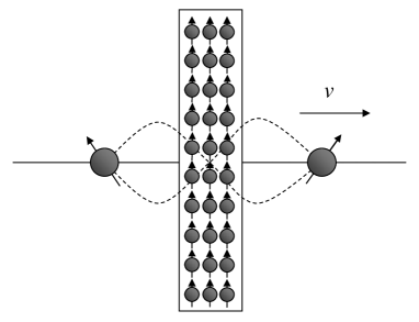
Figure 1: Schematic diagram of two electron spins going through a quantum well consisting of nuclear spins. Two electrons initially located at $z_{0}^{(1,2)}$ move with a uniform speed $v$.

We consider a system illustrated in Fig.1. Two electrons go through a quantum well one after the other. The electron spins described by Gaussian packets with width $a/2$ are initially located at $z_{0}^{(i)}$ ($i=1,2$) and move along the z-direction with a uniform speed $v$. The 2D quantum well consists of many polarized nuclear spins located in position $(x_{j},y_{j},z_{j})$ with $\left|x_{i}\right|\leq a$, $\left|y_{i}\right|\leq a$, $\left|z_{i}\right|\leq a/5$. When a static magnetic field is applied to the total system, the Hamiltonian reads as

$$H^{S}= \Omega_{z}(S_{z}^{(1)}+S_{z}^{(2)})+\omega_{z}\sum_{i}I_{z}^{(i)}$$

$$+S_{z}^{(1)}\sum_{i}g_{1}^{(i)}I_{z}^{(i)}+S_{z}^{(2)}\sum_{i}g_{2}^{(i)}I_{z}^{(i)}$$

$$+S_{+}^{(1)}\sum_{i}\frac{g_{1}^{(i)}}{2}I_{-}^{(i)}+S_{+}^{(2)}\sum_{i}\frac{g_{2}^{(i)}}{2}I_{-}^{(i)}+h.c.\text{,}$$ (1)

where $S_{z}^{(l)}$ and $S_{\pm}^{(l)}$ ($=S_{x}^{(l)}\pm iS_{y}^{(l)}$) ($l=1,2$) are the spin operators for the $l$’th electron spin, $I_{z}^{(j)}$ and $I_{\pm}^{(j)}$ ($=I_{x}^{(j)}\pm iI_{y}^{(j)}$) ($j=1,2,\cdots,N$) the spin operators for the $j$’th nuclear spin, $g_{l}^{(j)}$ ($l=1,2$, $j=1,2,\cdots,N$) the hyperfine coupling constants between $l$’th electron and $j$’th nuclear spin. The first and second terms of Hamiltonian (1) are the Zeeman energies for the electron spins and the nuclear spins respectively, and the terms besides them are the hyperfine interaction between the electrons and nuclear spins.

In our setup, the nuclear spins are restricted in a flat square box with $\left|x_{i}\right|\leq a$, $\left|y_{i}\right|\leq a$, $\left|z_{i}\right|\leq a/5$. We have (for the necessary details please refer to the Appendix A)

$$g_{1}^{(i)}\simeq g_{0}^{(i)}f_{1}(t)\text{, \ }g_{2}^{(i)}\simeq g_{0}^{(i)}f_{2}(t)\text{.}$$ (2)

In Ref. Song , the collective excitation of an ensemble of polarized nuclei fixed in a quantum dot was studied. Under the approximately homogeneous condition the many-particle system behaves as a single-mode boson interacting with the spin of a single conduction-band electron confined in this quantum dot. Likewise, we introduce a collective operator

$$B=\frac{\sum\nolimits_{i=1}^{N}g_{0}^{(i)}I_{-}^{(i)}}{\sqrt{2I_{0}\sum_{j}[g_{0}^{(i)}]^{2}}}$$

and its conjugate $B^{+}$ to depict the collective excitations in the ensemble of nuclei with spin $I_{0}$ from its polarized initial state

$$\left|G\right\rangle=\prod_{i=1}^{N}\left|-I_{0}\right\rangle_{i}$$

which is the saturated ferromagnetic state of nuclear ensemble. In our model, the nuclear spins are fixed in GaAs crystal lattice with $I_{0}=3/2$, $a=4nm$ and the density of nuclei $n_{0}=45.6nm^{-3}$. For simplicity, we assume the nuclei are located in a simple cubic lattice. Thus, we have the average distance between two neighboring nuclear spins $d=0.28nm$, $g_{max}^{2}/\overline{g^{2}}\simeq 11.7$, $N=5046$, where $g_{max}$ is the maximum of $g_{0}^{(i)}$ and $\overline{g^{2}}=\sum_{i}(g_{0}^{(i)})^{2}/N$. On condition that the number of excitations in the system $n\ll NI_{0}\overline{g^{2}}/g_{max}^{2}$, we have $[B,B^{+}]\rightarrow 1$. In other words, the collective excitation described by $B$ can behave as a boson mode in the large $N$ limit with an initial polarization of all spins in ground (spin down) state.

In addition to the basic mode denoted by $B$ and $B^{+}$, there exist auxiliary modes

$$C_{k}=\frac{\sum\nolimits_{i=1}^{N}h_{i}^{[k]}I_{-}^{(i)}}{\sqrt{2I_{0}(\vec{h}^{[k]})^{2}}}$$

for $k=1,2,\ldots,N$. Here,

$$\vec{h}^{[k]}=(h_{1}^{[k]},h_{2}^{[k]},\ldots,h_{N}^{[k]})$$

are $N$ orthogonal vectors in $N$-dimensional space $\mathbf{R^{N}}$, which can be systematically constructed by making use of the Gram-Schmidt orthogonalization method Gram-Schmidt starting from

$$\vec{h}^{[1]}=(g_{0}^{(1)},g_{0}^{(2)},\ldots,g_{0}^{(N)})\in\mathbf{R^{N}}.$$

Therefore, the Hamiltonian (1) is rewritten as

$$H^{S}\simeq (\Omega_{z}-f_{1}I_{0}\sum_{i}g_{0}^{(i)})S_{z}^{(1)}+(\Omega_{z}-f_{2}I_{0}\sum_{i}g_{0}^{(i)})S_{z}^{(2)}$$

$$+f_{1}\Omega(S_{+}^{(1)}B+S_{-}^{(1)}B^{+})+f_{2}\Omega(S_{+}^{(2)}B+S_{-}^{(2)}B^{+})$$

$$+\omega_{z}\sum_{k}C_{k}^{+}C_{k}+\omega_{z}B^{+}B+H_{p}^{S}$$ (3)

Here, the effective Rabi frequency

$$\Omega=\sqrt{\frac{1}{2}I_{0}\sum\nolimits_{i=1}^{N}\left[g_{0}^{(i)}\right]^{2}}\text{.}$$

describes the enhanced coupling of the electron spin to the collective excitations. And the single particle excitation term

$$H_{p}^{S}=(S_{z}^{(1)}f_{1}+S_{z}^{(2)}f_{2})\sum_{i}g_{0}^{(i)}(I_{z}^{(i)}+I_{0})$$ (4)

can be treated as a perturbation term in the low-excitation limit, which originates from the inhomogeneity of the couplings.

III Effective Inter-Spin Coupling Description

As shown in Hamiltonian (3), there are only couplings of two electron spins with the single mode boson respectively. By making use of the canonical transformation Li , we can eliminate the boson operator and obtain the effective interaction between the two electron spins. Former research mainly focused on the case where $f_{1}(t)\Omega$ and $f_{2}(t)\Omega$ are time independent Zheng . However,the time-independent approach may not work well in practice. Now, because of the motion of the electrons, we take the time-dependence of interaction into consideration, namely, $f_{1}(t)\Omega$ and $f_{2}(t)\Omega$ depend on time.

Let us first summarize the main idea of the time-dependent Fröhlich transformation Li so that our paper is self consistent for reading. Generally speaking, Fröhlich transformation Frohlich ; Nakajima is frequently used in condensed matter physics to obtain effective interaction between two electrons by exchanging virtual phonons. For a quantum system described by Hamiltonian $H(t)=H_{0}+H_{1}(t)$, where $H_{0}$ is time independent and $|H_{0}|\gg|H_{1}(t)|$, we can make a canonical transformation

$$|\psi(t)\rangle\rightarrow e^{-F(t)}|\psi(t)\rangle,\text{ \ }H(t)\rightarrow e^{-F(t)}H(t)e^{F(t)},$$ (5)

where $F(t)$ is an anti-Hermitian operator and $\psi(t)$ the state of the system. When $F(t)$ is appropriately chosen to make the first-order term of the effective Hamiltonian vanishing, i.e., $H_{1}+[H_{0},F]-i\partial_{t}F=0$, we obtain an effective Hamiltonian to the second order $H_{eff}=H_{0}+[H_{1},F]/2$ in principle, and the above equation explicitly determines $F=F(t)$.

In this section, the canonical transformations are made to obtain the effective Hamiltonian. In the interaction picture with respect to

$$H_{0}^{S}=\omega_{z}(S_{z}^{(1)}+S_{z}^{(2)})+\omega_{z}(B^{+}B+\sum_{k}C_{k}^{+}C_{k}),$$

the Hamiltonian $H^{I}=H_{0}^{I}+H_{1}^{I}+H_{p}^{I}$ contains three parts

$$H_{0}^{I}=\Delta_{1}S_{z}^{(1)}+\Delta_{2}S_{z}^{(2)}\text{,}$$ (6)

$$H_{1}^{I}=\sum_{i=1,2}f_{i}\Omega(S_{+}^{(i)}B+S_{-}^{(i)}B^{+})\text{,}$$ (7)

$$H_{p}^{I}=e^{itH_{0}^{S}}H_{p}^{S}e^{-itH_{0}^{S}}\equiv H_{p}^{S}$$ (8)

Here,

$$\Delta_{j}=\Omega_{z}-\omega_{z}+f_{j}I_{0}\sum_{i}g_{0}^{(i)}(j=1,2)$$

are the detunings of electron spin and nuclear spin and hyperfine interaction.

It can be observed from the Hamiltonian $H^{I}$ that the time-dependent term $H_{1}^{I}$ can be considered as first-order perturbation with respect to the zeroth-order term $H_{0}^{I}$ (disregarding $H_{p}^{I}$). Then, we perform a transformation $\exp(F(t))$ to the Hamiltonian $H^{I}$ to eliminate the time-dependent term $H_{1}^{I}$, that is, the condition

$$H_{1}^{I}+[H_{0}^{I},F]-i\partial_{t}F=0$$ (9)

should be fulfilled, where TDFT operator is

$$F(t)=(x_{1}(t)S_{+}^{(1)}+x_{2}(t)S_{+}^{(2)})B-h.c.$$

It follows from Eq. (9) that the corresponding coefficients of $S_{+}^{(1)}B$, $S_{-}^{(1)}B^{+}$, $S_{+}^{(2)}B$ and $S_{-}^{(2)}B^{+}$ at the left hand side of Eq. (9) vanish, i.e.,

$$f_{1}\Omega+\Delta_{1}x_{1}-i\dot{x}_{1} =0\text{,}$$ (10)

$$f_{2}\Omega+\Delta_{2}x_{2}-i\dot{x}_{2} =0\text{.}$$ (11)

In case that the electrons go through the nuclear spins with a uniform speed $v$, the solutions to the above equations are $x_{j}\simeq-f_{j}\Omega/\Delta$ ($j=1,2$), where $\Delta=\Omega_{z}-\omega_{z}$ is used to replace $\Delta_{1}$ and $\Delta_{2}$ since $\Delta\simeq\Delta_{1}\simeq\Delta_{2}$ in the realistic parameters (for the necessary details please refer to Appendix B). Then, the effective Hamiltonian is obtained approximately as follows

$$H^{F}\simeq H_{0}^{I}+\frac{1}{2}[H_{1}^{I},F]+H_{p}^{I}+[H_{p}^{I},F]$$

$$\simeq [\Delta_{1}-\frac{f_{1}^{2}\Omega^{2}}{\Delta}(2<B^{+}B>+1)]S_{z}^{(1)}$$

$$+[\Delta_{2}-\frac{f_{2}^{2}\Omega^{2}}{\Delta}(2<B^{+}B>+1)]S_{z}^{(2)}$$ (12)

$$-\frac{f_{1}f_{2}\Omega^{2}}{\Delta}[S_{+}^{(1)}S_{-}^{(2)}+S_{+}^{(2)}S_{-}^{(1)}]+H_{p}^{I}+[H_{p}^{I},F]\text{,}$$

where $\left\langle B^{+}B\right\rangle$ denotes the average number of nuclear excitation, and the fast-oscillating terms including the factor $exp(\pm i\Delta t)$ have been dropped off.

When almost all nuclear spins are in their ground state, the system is in the low collective excitation limit, i.e., $\left\langle B^{+}B\right\rangle\rightarrow 0$. By using

$$|\Delta_{1,2}|\simeq|\Delta|\gg f_{1,2}\Omega\text{,}$$

we have

$$\Delta_{j}-\frac{f_{j}^{2}\Omega^{2}}{\Delta}(2<B^{+}B>+1)\simeq\Delta_{j}\simeq\Delta\text{.}$$

Thus,

$$H^{F}\simeq \Delta(S_{z}^{(1)}+S_{z}^{(2)})-\frac{f_{1}f_{2}\Omega^{2}}{\Delta}(S_{+}^{(1)}S_{-}^{(2)}+h.c.)$$

$$+H_{p}^{I}+[H_{p}^{I},F]\text{.}$$ (13)

In the following calculation, it will be shown that the complex term $[H_{p}^{I},F]$ will be dropped in the interaction picture. With respect to $H_{0}=\Delta(S_{z}^{(1)}+S_{z}^{(2)})$, the effective interaction Hamiltonian is

$$H_{eff}=V_{1}+V_{2}\text{,}$$ (14)

where

$$V_{1} =-e^{iH_{0}t}[\frac{f_{1}f_{2}\Omega^{2}}{\Delta}(S_{+}^{(1)}S_{-}^{(2)}+S_{+}^{(2)}S_{-}^{(1)})]e^{-iH_{0}t}$$

$$=-\frac{f_{1}f_{2}\Omega^{2}}{\Delta}(S_{+}^{(1)}S_{-}^{(2)}+S_{+}^{(2)}S_{-}^{(1)})\text{,}$$ (15)

$$V_{2} =e^{itH_{0}}H_{p}^{I}e^{-itH_{0}}=H_{p}^{S}\text{.}$$ (16)

In the above calculation, we have dropped the high-frequency terms $\exp(iH_{0}t)[H_{p}^{I},F]\exp(-iH_{0}t)$ including the factors $\exp(\pm i\Delta t)$. It is a reasonable approximation which is frequently used in the Jaynes-Cummings model.

Now, we study the time evolution driven by the above effective Hamiltonian. First of all, we study a special case that the total system is initially prepared without the collective excitations of the bus spins. In this case, the effective interaction $V_{2}$ does not play a role. In a Hilbert space spanned by the two electron states $\left|ee\right\rangle$, $\left|eg\right\rangle$, $\left|ge\right\rangle$ and $\left|gg\right\rangle$, it is clear that there exists an invariant subspace spanned by $\left|eg\right\rangle$ and $\left|ge\right\rangle$. If the system starts from $\left|\Psi(0)\right\rangle=\left|eg\right\rangle$, at time $t$ it would definitely evolve into

$$\left|\psi(t)\right\rangle=\cos\theta(t)\left|eg\right\rangle-i\sin\theta(t)\left|ge\right\rangle,$$

where

$$\theta(t)=-\int_{0}^{t}\frac{f_{1}f_{2}\Omega^{2}}{\Delta}dt^{\prime}\text{.}$$ (17)

In comparison with the result in Ref. Song , where $H_{p}$ was considered as a perturbation in the low excitation approximation, we examine the system evolving under total Hamiltonian containing $V_{1}$ and $V_{2}$. Then we can get the equations for the coefficients as follow

$$i\dot{C}_{ge} =-\frac{f_{1}f_{2}\Omega^{2}}{\Delta}C_{eg}-(V_{2})_{eg}C_{ge}\text{,}$$ (18)

$$i\dot{C}_{eg} =(V_{2})_{eg}C_{eg}-\frac{f_{1}f_{2}\Omega^{2}}{\Delta}C_{ge}\text{,}$$ (19)

where $(V_{2})_{jk}=\langle jk|V_{2}\left|jk\right\rangle$ and $j,k=e,g$. Similarly, there’s an invariant subspace $\{\left|eg\right\rangle\text{,}\left|ge\right\rangle\}$.

IV Spin Entanglement

In the above sections, we have obtained a typical spin-spin coupling in the effective Hamiltonian, which is induced by the collective excitations. Driven by this Hamiltonian, two electron spins can be entangled dynamically. To characterize the extent of entanglement, we use concurrence to measure the induced entanglement. For an arbitrary state of two-qubit system described by the density operator $\rho$, a measure of entanglement can be defined as the concurrence Wootters ; Wang ,

$$C(\rho)=max\{0,\lambda_{1}-\lambda_{2}-\lambda_{3}-\lambda_{4}\}\text{,}$$ (20)

where the $\lambda_{i}$’s are the square roots of the eigenvalues of the non-Hermitian matrix $\rho\widetilde{\rho}$ in decreasing order. And

$$\widetilde{\rho}=(\sigma_{y}\otimes\sigma_{y})\rho^{\ast}(\sigma_{y}\otimes\sigma_{y}),$$

where $\rho^{\ast}$ is the complex conjugate of $\rho$, $\sigma_{y}$ the Pauli operator. Actually, even  from the original Hamiltonian (1) we can also prove that the corresponding reduced density matrix for two spin is of the form

$$\rho^{(12)}=\left(\begin{array}[]{cccc}u^{+}&0&0&0\\ 0&w^{1}&z^{\ast}&0\\ 0&z&w^{2}&0\\ 0&0&0&u^{-}\end{array}\right).$$ (21)

To prove the above result, we consider that, in the original Hamiltonian the interaction terms

$$H_{I}= S_{z}^{(1)}\sum_{j=1}^{N}g_{1}^{(j)}I_{z}^{(j)}+S_{z}^{(2)}\sum_{j=1}^{N}g_{2}^{(j)}I_{z}^{(j)}$$

$$+S_{+}^{(1)}\sum_{l=1}^{N}\frac{g_{1}^{(j)}}{2}I_{-}^{(j)}+S_{+}^{(2)}\sum_{j=1}^{N}\frac{g_{2}^{(j)}}{2}I_{-}^{(j)}+h.c.\text{,}$$ (22)

conserves the total spin z-component

$$\mathcal{S}_{z}=\sum_{j=1}^{N}I_{z}^{(j)}+S_{z}^{(1)}+S_{z}^{(2)}$$

i.e., $[H_{I},\mathcal{S}_{z}]=0$. For such conserved system we express the concurrence characterizing quantum entanglement in terms of observables, such as correlation functions.

The complete basis vectors of the total system are denoted by

$$|S_{1},S_{2},\{I_{j}\}\rangle = |S_{1},S_{2};I_{1},..,I_{N}\rangle$$ (23)

$$= \prod\limits_{j=1}^{N}|I_{j}\rangle\otimes|S_{1}\rangle\otimes|S_{2}\rangle$$

where $|I_{j}\rangle$ is nuclear spin state and $|S_{1,2}\rangle$ denote the electronic spins$\ \ (I_{j},S_{1,2}=0,1)$ respectively. The fact that $\mathcal{S}_{z}$ is conserved can be reflected by the vanishing of some matrix elements of the density operator $\rho=\rho(H)$ on the above basis for any state of the total system, that is,

$$\rho_{S_{1},S_{2};I_{1},..,I_{N}}^{S_{1}^{\prime},S_{2}^{\prime};I_{1}^{\prime},..,I_{N}^{\prime}}=\rho_{\{n_{j},s_{j}\}}^{\{n_{j},s_{j}\}}\delta(s,s^{\prime},I,I^{\prime}),$$ (24)

where

$$\delta(s,s^{\prime},I,I^{\prime})=\delta(S_{1}+S_{2}-S_{1}^{\prime}-S_{2}^{\prime}+\sum_{j=1}^{N}(I_{j}-I_{j}^{\prime}))$$

The functional $\rho(H)$ of the Hamiltonian may be a ground state or thermal equilibrium states. The reduced density matrix $\rho^{(12)}=Tr_{I}[\rho(H)]$ for two spins, e.g., $S_{1}$ and $S_{2}$ are obtained as

$$[\rho^{(12)}]_{S_{1},S_{2};}^{S_{1}^{\prime},S_{2}^{\prime};}=\delta(s,s^{\prime},0,0)\sum_{\{I_{j}\}}\rho_{S_{1},S_{2};I_{1},..,I_{N}}^{S_{1}^{\prime},S_{2}^{\prime};I_{1},..,I_{N}}$$ (25)

by tracing over all nuclear variables. The corresponding reduced density matrix for two spins $1$ and $2$ is of the form in Eq.(21). Using the observable quantities, the quantum correlation

$$z = \left\langle\psi\right|S_{1}^{+}S_{2}^{-}\left|\psi\right\rangle,$$ (26)

$$u^{\pm} = \left\langle\psi\right|\left(1/2\pm S_{1}^{z}\right)\left(1/2\pm S_{2}^{z}\right)\left|\psi\right\rangle,$$

the concurrence is rewritten as a computable form

$$C_{12}=2\max(0,\left|z\right|-\sqrt{u^{+}u^{-}}).$$ (27)

We note that this formula for the concurrence of two electron spins in the coupled system is the same as that for a spin-1/2 coupling system modeled by the effective Hamiltonian Wootters ; Wang . This general form is consistent with that obtained straightforwardly from the effective Hamiltonian given in the last section.

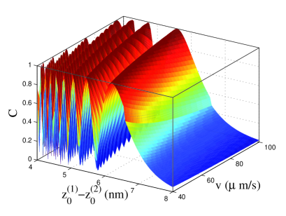
Figure 2: (Color Online) The relation between concurrence $C$ and velocity $v$, distance $z_{0}^{(1)}-z_{0}^{(2)}$, on condition that $a=4$ nm, $\Delta=8\times 10^{11}$ Hz, $I_{0}=3/2$, $n=0$.

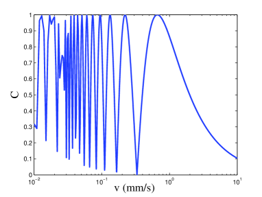
Figure 3: Cross section of Fig.2 with $z_{0}^{(1)}-z_{0}^{(2)}=4$ nm.

With the above general consideration, we now study quantitatively the concurrence for the quantum entanglement of the two electrons passing the nuclear spins at a uniform speed $v$. In Fig. 2, the concurrence is plotted while the speed $v$ and the initial distance between the two electrons $z_{0}^{(1)}-z_{0}^{(2)}$ are varied. It is obvious that the concurrence fluctuates from $0$ to $1$ in the low speed region (see also Fig. 3). When the electrons move with a relative low speed, the concurrence oscillates rapidly since a lower speed means more time for evolution from a direct product state towards an entangled state. As the speed increases, the concurrence falls monotonously if it is bigger than a certain value. According to Eq. (17), the maximum entangled state can be obtained when

$$\theta=(n+1)\frac{\pi}{4}\text{.}$$ (28)

However, the general relation between the concurrence and $z_{0}^{(1)}-z_{0}^{(2)}$ is a little more complicated. The further the two electrons separate from each other, the longer time both of them need to pass through the nuclear ensemble. On the other hand, the matrix elements of the effective interaction $V_{1}$ in Eq. (15), i.e., $\langle\uparrow\downarrow|V_{1}|\downarrow\uparrow\rangle$, h.c., drop dramatically as the inter-spin distance increases. This observation is obviously correct from an intuitively physical consideration. For a longer inter-spin distance, the spatial wave function of two spins has a smaller overlap, and then the effective coupling is weak.

In the last section, we have only taken $V_{1}$ into consideration. However, due to the nuclear excitation, i.e., $n>0$, $V_{2}$ will lead to decoherence. According to Ref. Song , under the quasihomogeneous condition, we have $\sum_{i}g_{0}^{(i)}(I_{z}^{(i)}+I_{0})=n\overline{g}$, where $\overline{g}=\sum_{i}g_{0}^{(i)}/N$, $n=\langle B^{+}B\rangle$ is the average number of collective excitation. Thus, the single particle perturbation can be approximated as

$$V_{2}=H_{p}^{S}\simeq n\overline{g}(f_{1}S_{z}^{(1)}+f_{2}S_{z}^{(2)})\text{.}$$ (29)

In Fig. 4, we plot the concurrence evolution under $H_{eff}=V_{1}+V_{2}$. As shown in the figure, the two spins evolve into a maximum entangled state with appropriate parameters when $n=0$. On the contrary, the concurrence is suppressed when there exists collective excitation in the nuclei. Moreover, as more nuclei are excited, the concurrence falls dramatically.

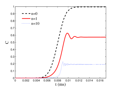
Figure 4: (Color Online) The evolution of concurrence $C$ on condition that $a=4$ nm, $\Delta=8\times 10^{11}$ Hz, $I_{0}=3/2$, $v=0.7$ mm/s.

V Conclusion

In summary, we have proposed a scheme to entangle two electron spins via an ensemble of nuclei. We also explore the influence of its collective excitation on the concurrence characterizing two spin entanglement. Theoretically, the maximum entangled state can be obtained if the electrons move in a suitable way. Furthermore, with the optimized experimental parameters, the operation time is within the relaxation time of electron spins in solid state systems, i.e., the order of ms Elzerman .

However, this scheme may encounter some difficulties in practice since it is based on the low excitation requirement of nuclear ensemble. In recent experiments, the number of excitation $n$ is of the order of $60\%N$ Bracker . Thus, further progress in experiment, i.e., lowering the temperature or optical excitation, are expected to prepare all nuclear spins in their ground states in order to put this scheme into practice. Actually, there are only the collective excitations considered as the quantum data bus to coherently link two spins so that the inter-spin entanglement is induced. If there exists noncollective excitations, then extra decoherence will be induced to break our scheme presented in this paper. Further investigations are needed for these questions. However, if we can cool the nuclear ensemble via some new mechanism, e.g., similar to Ref.Zhang ; Coolexpts , our scheme will probably work well.

Appendix A Derivation of $g_{1}^{(i)}$ and $g_{2}^{(i)}$

According to Ref.Schliemann , the hyperfine interaction constant is mainly proportional to the electron spin density located at the nucleus. Thus,

$$g_{1}^{(i)}=\frac{4\mu_{0}}{3I_{0}\hbar}\mu_{B}\mu_{I}\left|\psi_{1}^{(i)}\right|^{2}\text{,}$$ (30)

where $\mu_{0}$ is vacuum permeability, $I_{0}$ total nuclear spin quantum number, $\mu_{B}$ the Bohr magneton, $\mu_{I}$ the nuclear magnetic moment, $\psi_{1}^{(i)}$ the wavefunction for electron 1 located at the $i$’th nuclear spin. In a semiconductor crystal, the wavefunction is given by the product of the Bloch amplitude $u(\vec{r})$ and an envelope function $\Psi(\vec{r})$, i.e., $\psi(\vec{r})=u(\vec{r})\Psi(\vec{r})$. In a realistic crystal $\eta=\left|u(\vec{r})\right|^{2}$ reaches a climax at the lattice positions. It was discovered that $\eta_{As}=4.5\times 10^{3}$ and $\eta_{Ga}=2.7\times 10^{3}$ Paget . On account of isotope abundance and their different nuclear magnetic moment AIPH , $\overline{\mu_{I}\eta}=3.153\times 10^{-23}A\cdot m^{2}$. In our simulation, we assume that the wavefunction is Gaussian wave packet with initial location $z_{i}^{(1)}$ and a uniform speed $v$, that is

$$\left|\psi_{1}^{(i)}\right|^{2}=\left(\frac{4}{\pi a^{2}}\right)^{3/2}e^{-4[x_{i}^{2}+y_{i}^{2}+(z_{0}^{(1)}+vt-z_{i})^{2}]/a^{2}}\text{,}$$ (31)

where $\vec{r}_{i}=x_{i}\hat{x}+y_{i}\hat{y}+z_{i}\hat{z}$ is the position of the $i$’th nuclear spin with respect to the center of nuclei.

Since the nuclei are distributed in a flat box with $\left|x_{i}\right|\leq a$, $\left|y_{i}\right|\leq a$, $\left|z_{i}\right|\leq a/5$. Therefore,

$$g_{1}^{(i)} \simeq\frac{4\mu_{0}}{3I_{0}\hbar}\mu_{B}\mu_{I}\eta\left(\frac{4}{\pi a^{2}}\right)^{3/2}e^{-4r_{i}^{2}/a^{2}}e^{-4(z_{0}^{(1)}+vt)^{2}/a^{2}}$$

$$=g_{0}^{(i)}f_{1}(t)\text{,}$$ (32)

where

$$g_{0}^{(i)} =\frac{4\mu_{0}}{3I_{0}\hbar}\mu_{B}\mu_{I}\eta\left(\frac{4}{\pi a^{2}}\right)^{3/2}e^{-4r_{i}^{2}/a^{2}}\text{,}$$ (33)

$$f_{1}(t) =e^{-4(z_{0}^{(1)}+vt)^{2}/a^{2}}\text{.}$$ (34)

Here, we have neglected the term $e^{-8(z_{0}^{(1)}+vt)z_{i}/a^{2}}$ based on the following consideration. On the one hand, the above approximation tends to be exact as the quasi-2D quantum well becomes narrower in the z-direction, e.g., $\left|z_{i}\right|\rightarrow 0$. On the other hand, the effective coupling intensity is increased as more nuclear spins are included when $\left|z_{i}\right|$ get larger. Thus, optimal value is chosen for the valid approximation. Similarly, we have

$$g_{2}^{(i)}\simeq g_{0}^{(i)}f_{2}(t)\text{,}$$ (35)

where

$$f_{2}(t)=e^{-4(z_{0}^{(2)}+vt)^{2}/a^{2}}\text{.}$$ (36)

Appendix B Derivation of $x_{i}$

According to Eq.(10), one has

$$x_{1} =-i\Omega e^{-i\int_{0}^{t}\Delta_{1}dt^{\prime}}\int_{0}^{t}f_{1}e^{i\int_{0}^{t^{\prime}}\Delta_{1}dt^{\prime\prime}}dt^{\prime}$$

$$\simeq-i\Omega e^{-i\Delta t}\int_{-\infty}^{t}f_{1}e^{i\Delta t^{\prime}}dt^{\prime}$$

$$=\frac{-\Omega}{\Delta}e^{-i\Delta t}[f_{1}e^{i\Delta t}-\frac{8v}{a^{2}}\int_{-\infty}^{t}f_{1}e^{i\Delta t^{\prime}}(z_{0}^{(1)}+vt^{\prime})dt^{\prime}]$$

$$\simeq\frac{-\Omega}{\Delta}e^{-i\Delta t}(f_{1}e^{i\Delta t}-\frac{8v}{a}\int_{-\infty}^{t}f_{1}e^{i\Delta t^{\prime}}dt^{\prime})\text{.}$$

Here, we have replaced $\Delta_{1}$ by $\Delta=\Omega_{z}-\omega_{z}$ since

$$f_{1}I_{0}\sum_{i}g_{0}^{(i)}\lesssim 8.318\times 10^{10}\text{ Hz}\ll\Delta=8\times 10^{11}\text{ Hz.}$$

Furthermore, we have replaced

$$\frac{8v}{a^{2}}\int_{-\infty}^{t}f_{1}e^{i\Delta t^{\prime}}[z_{0}^{(1)}+vt^{\prime}]dt^{\prime}$$

by

$$\frac{8av}{a^{2}}\int_{-\infty}^{t}f_{1}e^{i\Delta t^{\prime}}dt^{\prime}\text{,}$$

since one notices the fact that $z_{0}^{(1)}+vt^{\prime}\sim a$ is the effective integration range and the change of $f_{1}(t^{\prime})$ (also change of $vt^{\prime}$) is much slower than that of $e^{i\Delta t^{\prime}}$. Thus,

$$x_{1} \simeq\frac{-\Omega}{\Delta}f_{1}-i\frac{8v}{\Delta a}x_{1}\text{,}$$

Generally speaking, $\Delta$ depends on the applied magnetic field. In case that $\Delta=8\times 10^{11}$ Hz and $a\thicksim 4$nm, we have $8v/a\Delta\ll 1$ for all $v\ll 400$ m/s. Thus, we have

$$x_{1} \simeq\frac{-\Omega}{\Delta}f_{1}\text{.}$$ (37)

Similarly,

$$x_{2} \simeq\frac{-\Omega}{\Delta}f_{2}\text{.}$$ (38)

References

• (1) P. W. Shor, in Proceedings of the Symposium on the Foundations of Computer Science, 1994, Los Alamitos, California (IEEE Computer Society Press, New York, 1994), pp. 124-134.
• (2) L. K. Grover, Phys. Rev. Lett. 79, 325-328 (1997).
• (3) G. L. Long, Phys. Rev. A 64, 022307 (2001).
• (4) D. Loss, and D. P. DiVincenzo, Phys. Rev. A 57, 120 (1998).
• (5) B. E. Kane, Nature 393, 133 (1998).
• (6) Nan Zhao, L. Zhong, Jia-Lin Zhu, and C. P. Sun, Phys. Rev. B. 74, 075307 (2006).
• (7) J. M. Taylor, C. M. Marcus, and M. D. Lukin, Phys. Rev. Lett. 90, 206803 (2003).
• (8) J. M. Taylor, A. Imamoglu,, and M. D. Lukin, Phys. Rev. Lett. 91, 246802 (2003).
• (9) G. L. Long, Y. J. Ma, and H. M. Chen, Chin. J. Semiconductor, 24, Suppl. May, 43 (2003).
• (10) G. P. Berman, G. W. Brown, M. E. Hawley, and V. I. Tsifrinovich, Phys. Rev. Lett. 87, 097902 (2001).
• (11) Qing Ai, Y. Li, G. L. Long, and C. P. Sun, (unpublished).
• (12) Z. Song, P. Zhang, T. Shi, and C. P. Sun, Phys. Rev. B 71, 205314 (2005).
• (13) Yong Li, C. Bruder, and C. P. Sun, Phys. Rev. A 75, 032302 (2007).
• (14) J. P. Gram, Journal. für die reine und angewandte Math., 94, 71 (1883); E. Schmidt, Math. Ann., 63, 433 (1907).
• (15) S.-B. Zheng and G.-C. Guo, Phys. Rev. Lett. 85, 2392 (2000).
• (16) H. Fröhlich, Phys. Rev. 79, 845 (1950); Proc. Roy. Soc. A 215, 291 (1952); Adv. Phys. 3, 325 (1954).
• (17) S. Nakajima, Adv. Phys. 4, 463 (1953).
• (18) W. K. Wootters, Phys. Rev. Lett. 80, 2245 (1998).
• (19) X. Wang and P. Zanardi, Phys. Lett. A 301, 1 (2002); X. Wang, Phys. Rev. A 66, 034302 (2002).
• (20) J. M. Elzerman, R. Hanson, L. H. Willems van Beveren, B. Witkamp, L. M. K. Vandersypen, and L. P. Kouwenhoven, Nature 430, 431 (2004).
• (21) Bracker, A. S., E. A. Stinaff, D. Gammon, M. E. Ware, J. G. Tischler, A. Shabaev, A. L. Efros, D. Park, D. Gershoni, V. L. Korenev, and I. A. Merkulov, Phys. Rev. Lett. 94, 47402 (2005).
• (22) P. Zhang, Y. D. Wang, and C. P. Sun, Phys. Rev. Lett. 95, 097204 (2005).
• (23) J. Schliemann, A. Khaetskii, and D. Loss, J. Phys.: Condens. Matter 15, R1809 (2003).
• (24) D. Paget, G. Lampel, B. Sapoval, and V. Safarov, Phys. Rev. B 15, 5780 (1977).
• (25) American Institue of Physics Handbook, 3rd edn, (McGraw-Hill, New York, 1972).
• (26) D. Kleckner and D. Bouwmeester, Nature 444, 75 (2006); A. Naik, O. Buu, M. D. LaHaye, A. D. Armour, A. A. Clerk, M. P. Blencowe, and K. C. Schwab, Nature 443, 193 (2006); S. Gigan, H. R. Böhm, M. Paternostro, F. Blaser, G. Langer, J. B. Hertzberg, K. C. Schwab, D. Bäuerle, M. Aspelmeyer, and A. Zeilinger, Nature 444, 67 (2006); O. Arcizet, P.-F. Cohadon, T. Briant, M. Pinard, and A. Heidmann, Nature 444, 71 (2006); M. Poggio, C. L. Degen, H. J. Mamin, and D. Rugar, cond-mat/0702446.