Statistics of Measurement of Non-commuting Quantum Variables:
Monitoring and Purification of a qubit

Abstract

We address continuous weak linear quantum measurement and argue that it is best understood in terms of statistics of the outcomes of the linear detectors measuring a quantum system, for example, a qubit. We mostly concentrate on a setup consisting of a qubit and three independent detectors that simultaneously monitor three non-commuting operator variables, those corresponding to three pseudo-spin components of the qubit. We address the joint probability distribution of the detector outcomes and the qubit variables. When analyzing the distribution in the limit of big values of the outcomes, we reveal a high degree of correspondence between the three outcomes and three components of the qubit pseudo-spin after the measurement. This enables a high-fidelity monitoring of all three components. We discuss the relation between the monitoring described and the algorithms of quantum information theory that use the results of the partial measurement.

We develop a proper formalism to evaluate the statistics of continuous weak linear measurement. The formalism is based on Feynman-Vernon approach, roots in the theory of full counting statistics, and boils down to a Bloch-Redfield equation augmented with counting fields.

I introduction

The theory of quantum measurement, being a foundation of quantum physics, is attracting more and more attention quantum-measure . Intrinsic paradoxes Leggett are definitely a main reason for studying quantum measurements. More motivation comes from the practical needs to understand the real solid-state based devices solid-state ; qubit-review developed for quantum computing quantum-computing . Measurements in solid-state setups may provide access to extra variables that facilitate the read out of the quantum information stored in the elementary two-level quantum systems (qubits). The concept of continuous weak linear measurement (CWLM), where the interaction between the detector and the measured system is explicit and sufficiently weak, has been recently elaborated in context of the solid state quantum computing Korotkov1 ; Averin ; Clerk ; Jordan ; Korotkov . CWLM provides a universal description of the measurement process and is based on general linear response theory point . It applies to a large class of linear detectors: From common amplifiers to more exotic on-chip detectors such as quantum point contact QPC , superconducting SET transistors SET , generic mesoscopic conductors MES , fluxons in a Josephson transmission line to measure a flux qubit ARS ; ARD .

It is an important feature of CWLM that the (quantum) information is transferred from a quantum system being measured — a qubit — to other degrees of freedom: those of the detector. The outcome of the measurement is thus represented by the detector degrees of freedom rather than those of the qubit. We will address both the statistics of the outcomes and joint statistics of the outcomes and the qubit degrees of freedom.

We stress the difference between the detector outcomes and the outcomes of a projective measurement of a qubit. In distinction from the result of a projective measurement, the detector outcome is not discrete, since the detector output (for instance, voltage or current) is a continuous variable. The outcomes do not even have to correlate with the state of the qubit if the detector is uncoupled. Further, the detector variables are subject to noise not related to the qubit. Owing to the feedback of the detector at the qubit, this noise affects the qubit too.

In comparison with the text-book projective measurement that instantly provides a result and projects the system onto the state corresponding to the result, the CWLM takes time both to accumulate the information and to distort the qubit. The time $\tau_{m}$ required to obtain a sufficiently accurate measurement result is called ”measurement time” and is a characteristic of a CWLM setup. It is not a duration of an individual measurement in this setup: the latter may vary. The distortion is due to the inevitable back action of the detector and is characterized by the dephasing rate $\Gamma_{d}$. It has been shown Korotkov1 ; Averin ; Clerk that for an optimized — quantum limited — detector $\tau_{m}\Gamma_{d}=1/2$ while the ”measurement time” $\tau_{m}$ greatly exceeds $1/2\Gamma_{d}$ for less optimal detectors.

In the context of quantum information theory, CWLM may be understood as an interaction of the qubit with infinitely many ancillary qubits representing the detector degrees of freedom. Each ancilla is brought to weakly interact with the qubit for a short time and is subsequently measured. Owing to the interaction, the quantum state of the ancillae is entangled with the state of the qubit. The detector output is proportional to the sum of the measurement results of a large set of ancillae. This allows to transfer quantum information from the qubit to the detector without formal projective measurement of the qubit. Therefore the peculiarities of the CWLM can be understood in the framework of a projective measurement, although a more complicated one involving the detector degrees of freedom. The CWLM can be thus seen as a build-up of an entanglement between the qubit and the detector. An outcome of an individual CWLM is the detector output accumulated during the time interval of a certain duration $\tau_{d}$. Any CWLM can be described as a generalized quantum measurement, that involves qubit and detector degrees of freedom.

The outcome randomly varies from measurement to measurement. We argue here that studying statistics of the measurement outcomes of a CWLM is the best way to understand and characterize such a measurement. This is especially important for the simultaneous measurement of non-commuting variables (say, $A$ and $B$) we concentrate on in this work. In this case, the text-book projective measurement can not help to predict the statistics of the results: it would depend on the order of measurements of $A$ and $B$. This property of the measurements in non-commuting bases enables most quantum cryptography crypt algorithms and has been extensively elucidated in Ref. Busch .

One can straightforwardly realize in experiment a CWLM of a quantum system where $A$ and $B$ are measured simultaneously. If $A$ and $B$ commute, the statistics of the outcomes of sufficiently long CWLM corresponds to the predictions of projective measurement scheme (see Sec. III). The projective measurement scheme loses its predictive power if $A$ and $B$ do not commute. The reason is that the order of measurement of $A$ and $B$ is not determined in the course of a continuous measurement. The statistics of CWLM outputs thus can not be straightforwardly conjectured and has to be evaluated from the quantum mechanical treatment of the whole system consisting of the qubit and the detectors.

In a sharp contrast to the case of commuting variables, the most probable outcome of a sufficiently long CWLM of non-commuting variables does not depend on the qubit state. Therefore it provides no information about the qubit. The information is however hidden in the statistics of random outcomes. Recently, the simultaneous acquisition of two non-communing observables was investigated in the framework of CWLM Jordan , and the correlation of the random output of two detectors was found to be informative. Not only noise, but the whole full counting statistics (FCS) of the non-commuting measurements has been recently addressed for an example of many spins traversing the detectors Lorenzo .

The structure of the article is as follows. We develop the necessary formalism in Sec. II. Our approach stems from the FCS theory of electron transfers Levitov in the extended Keldysh formalism Nazarov , which has been recently discussed Makhlin-Lesovik in the context of the quantum measurement. At first step, we obtain a Feynman-Vernon action to describe the fluctuations of the input and output variables of the detector(s). In the relevant limit, the action is local in time. So at the second step we reduce the path integral to the solution of a differential equation that appears to be a Bloch-Redfield equation augmented with the counting field. In Sec. III we exemplify the formalism addressing a relatively simple case of quantum non-demolition (QND) measurement QND . We evaluate the distribution of the outcomes for a single detector and understand the statistics of a recently proposed quantum un-demolition measurementKorotkov . The main results are presented in Sec. IV where we discuss statistics of measurement of non-commuting variables for the case of three independent detectors measuring the three components of the qubit pseudo-spin. We find the statistical correspondence between the three outcomes and three wavefunction components after the measurement. The correspondence is characterized by a fidelity that generally increases with the magnitude of the outcomes reaching the ideal value $1$ in the limit of large magnitudes. Since very large outcomes are statistically rare and require long waiting times, this result could be of a purely theoretical value. To prove the opposite, we have evaluated the fidelity at moderate magnitudes of outcomes and measurement durations $\tau_{d}$ and we were able to demonstrate the fidelity of $0.95$ for $\tau_{d}\simeq 7\tau_{m}$. We term this ”quantum monitoring”. Ideally, the result of the quantum monitoring is a pure state of the qubit and three numbers (detector outputs) giving the polarization of the state. The same result can be also achieved by preparing the qubit state of the known polarization, for instance, by a projective measurement along a certain axis. The difference is that in the case of preparation the polarization axis is known to the observer in advance, while in the case of monitoring it is not so: both the three numbers and the state emerge from dynamics of the quantum system that encompasses the qubit and the detectors.

We discuss the relation between the quantum monitoring proposed and the quantum algorithms that use the results of partial measurements that we summarize in Sec. V. We evaluate the detector action in the Appendix A. We prove in the Appendix B that our approach correspond to a Lindblad scheme for a system consisting of the detectors and the qubit.

II Method

We start the outline of the formalism with a simplest setup where a single detector measures a single component of the qubit pseudo-spin. In this case, the Hamiltonian reads as follows:

$$H = H_{q}+H_{int}+H_{d}\,,$$ (1a)

$$H_{q} = \sum\limits_{i=1}^{3}H_{i}\hat{\sigma}_{i};\;H_{int}=\hat{\sigma}_{3}\hat{Q}\,.$$ (1b)

Here, $H_{q}$ is the Hamiltonian of the qubit generally given by a linear combination of three Pauli matrices $\hat{\sigma}_{i}$ ($i=1$, $2$, $3$) corresponding to three components of the qubit pseudo-spin. $H_{int}$ gives the coupling between the detector and the third component of the pseudo-spin of the qubit, $\hat{Q}$ being the detector input variable. $H_{d}$ stands for the Hamiltonian of the detector. Since we assume linear dynamics of the detector variables, a general form of this Hamiltonian is that of a boson bath,

$$H_{d}=\sum_{k}\hbar\omega_{k}\hat{b}_{k}^{\dagger}\hat{b}_{k}.$$

This encompasses infinitely many boson degrees of freedom labeled by $k$, $\hat{b}_{k}$ being the corresponding annihilation operators. The output of the detector is given by the output variable $\hat{V}$. An arbitrary linear dynamics is reproduced if both variables $\hat{Q}$ and $\hat{V}$ are linear combinations of the boson creation/annihilation operators,

$$\hat{Q} = \sum_{k}\left(Q_{k}\hat{b}^{\dagger}_{k}+Q^{*}_{k}\hat{b}_{k}\right)\,,$$ (2)

$$\hat{V} = \sum_{k}\left(V_{k}\hat{b}^{\dagger}_{k}+V^{*}_{k}\hat{b}_{k}\right).$$ (3)

This is in the spirit of Caldeira-Leggett approachCaldeira . In contrast to the work Caldeira we do not assume thermal equilibrium in the boson bath. In fact, this assumption would be wrong for most practical detectors since a signal amplification can not take place in the state of thermal equilibrium. The only requirement we impose is that Wick’s theorem holds for the boson operators involved. This guarantees the linear dynamics of the detector variables. Besides, this conveniently allows us not to specify the coefficients $Q_{k},V_{k}$. All information about the coefficients and the non-equilibrium boson distribution is incorporated into the two-point correlators of the variables explicitly given below (Eqs. 7-8). By virtue of Wick’s theorem, the averages of all possible products of the detector variables can be expressed in terms of these two-point correlators.

We are interested in the statistics of the detector output variable $\hat{V}$. We note that this variable is distinct from those of the qubit and in principle even does not have to correlate with the qubit state (e.g. if $\hat{Q}=0$). However, since the detector is supposed to measure the qubit, there must be a (high) degree of correspondence between the detector output and the qubit state. This sets the goal of our calculation: to access the joint statistics of $\hat{V}$ and the qubit variables.

To achieve the goal, we introduce a counting field $\chi(t)$ coupled to the output variable $\hat{V}$ and use a modified Feynman-Vernon scheme Feynman-Vernon where the evolution of the ”bra” and ”ket” wave function is governed by different Hamiltonians $H^{-}$ and $H^{+}$: $H^{\pm}=H\pm\hbar\chi(t)\hat{V}/2$. $\pm$ corresponds to two branches of closed time contour respectively Keldysh ; Rammer-Smith . This scheme was first employed in the work Nazarov-2 . The counting field $\chi(t)$ plays a role of the parameter in the generating function of the probability distribution of the detector outcomes $V(t)$. This generating function is given by:

$$Z(\{\chi(t)\})=\mathrm{Tr}\bigl{(}\overrightarrow{\mathrm{T}}e^{\frac{-i}{\hbar}\int dtH^{-}}\hat{\mathrm{R}}(0)\,\overleftarrow{\mathrm{T}}e^{\frac{i}{\hbar}\int dtH^{+}}\bigr{)}\,.$$ (4)

$\mathrm{Tr}(\cdots)$ implying the trace over both detector and qubit variables. Here, $\overrightarrow{\mathrm{T}}$($\overleftarrow{\mathrm{T}}$) denotes time (reversed) ordering in evolution exponents and $\hat{\mathrm{R}}(0)=\hat{\rho}_{d}(0)\bigotimes\hat{\rho}(0)$ is the initial density matrix of whole system. It separates into $\hat{\rho}_{d}(0)$ and $\hat{\rho}(0)$, the initial density matrix of the detector and qubit respectively. This implies that the detector and the qubit do not interact before the initial time moment $t=0$.

Next, we employ the path integral representation for the probability-generating function Nazarov-2 . According to Feynman and Vernon Feynman-Vernon (see also Kindermann ):

$$Z(\{\chi(t)\}) = \int\mathcal{D}{\bar{X}}^{+}\mathcal{D}{\bar{X}}^{-}e^{A_{d}}Z_{Iq}(Q^{-},Q^{+})\,,$$ (5)

here $\bar{X}^{\pm}(t)$ are two-dimensional vectors of the detector variables $\bar{X}^{\pm}(t)=(Q^{\pm}(t),V^{\pm}(t))^{T}$, $\mathcal{D}{\bar{X}}^{\pm}\equiv\prod\limits_{t}dQ^{\pm}(t)dV^{\pm}(t)$. $Q^{\pm}(t),V^{\pm}(t)$ are the path-integral variables. $Z_{Iq}$ is called the ”influence functional” and is given by

$$Z_{Iq}(Q^{-},Q^{+}) = \mathrm{Tr}_{\rm q}\bigl{(}\overrightarrow{\mathrm{T}}e^{-\frac{i}{\hbar}\int dt\,(H_{q}+\hat{\sigma}_{3}Q^{+}(t))}\hat{\mathrm{\rho}}(0)$$ (6)

$$\times\overleftarrow{\mathrm{T}}e^{\frac{i}{\hbar}\int dt\,(H_{q}+\hat{\sigma}_{3}Q^{-}(t))}\bigr{)}\,,$$

where $\mathrm{Tr}_{q}$ means the trace over qubit space. The action $A_{d}$ in Eq. (5) is bilinear in $\bar{X}^{\pm}$ and $\chi$ to conform to linear dynamics of the detector and will be specified below. The advantage of this representation is that the dynamics of infinitely many detector degrees of freedom have been reduced to the dynamics of only two relevant fields: $\hat{Q}$ and $\hat{V}$. The influence functional describes a non-linear response of the qubit on the fields.

Let us turn to a specific model of linear dynamics of the detector. Following common assumptions about CWLM, Averin ; Clerk we assume instant detector responses and white (frequency-independent) noises. Under these assumptions, a detector is characterized by seven independent parameters: four response functions and three noises. It is convenient to use an index $i$ taking values $1$ and $2$ for input and output variables respectively. With this index, we present $4$ response functions $a_{ij}$ as a single $2\times 2$ matrix. The noises $S_{ij}$ form a similar matrix. By virtue of Kubo formula, the response functions are expressed in terms of expectation values of the operator commutators

$$-\frac{i}{\hbar}\langle[\hat{Q}(t),\hat{Q}(t^{\prime})]\rangle = a_{11}\delta(t-t^{\prime}-0^{+})\,,$$ (7a)

$$-\frac{i}{\hbar}\langle[\hat{Q}(t),\hat{V}(t^{\prime})]\rangle = a_{12}\delta(t-t^{\prime}-0^{+})\,,$$ (7b)

$$-\frac{i}{\hbar}\langle[\hat{V}(t),\hat{Q}(t^{\prime})]\rangle = a_{21}\delta(t-t^{\prime}-0^{+})\,,$$ (7c)

$$-\frac{i}{\hbar}\langle[\hat{V}(t),\hat{V}(t^{\prime})]\rangle = a_{22}\delta(t-t^{\prime}-0^{+})\,,$$ (7d)

where an infinitesimal small positive number $0^{+}$ in the $\delta$-function represents small but finite response time.

The noises correspond to the expectation values of symmetrized operator products,

$$\langle\langle\frac{\hat{Q}(t)\hat{Q}(t^{\prime})+\hat{Q}(t^{\prime})\hat{Q}(t)}{2}\rangle\rangle = S_{11}\delta(t-t^{\prime})\,,$$ (8a)

$$\langle\langle\frac{\hat{V}(t)\hat{V}(t^{\prime})+\hat{V}(t^{\prime})\hat{V}(t)}{2}\rangle\rangle = S_{22}\delta(t-t^{\prime})\,,$$ (8b)

$$\langle\langle\frac{\hat{Q}(t)\hat{V}(t^{\prime})+\hat{V}(t^{\prime})\hat{Q}(t)}{2}\rangle\rangle = S_{12}\delta(t-t^{\prime})\,,$$ (8c)

$$\langle\langle\frac{\hat{V}(t)\hat{Q}(t^{\prime})+\hat{Q}(t^{\prime})\hat{V}(t)}{2}\rangle\rangle = S_{21}\delta(t-t^{\prime})\,,$$ (8d)

here, $\langle\langle\hat{A}\hat{B}\rangle\rangle\equiv\langle(\hat{A}-\langle\hat{A}\rangle)(\hat{B}-\langle\hat{B}\rangle)\rangle$ for any operators $\hat{A}$ and $\hat{B}$.

Let us discuss the physical meaning of the parameters involved. $S_{11}$ is the noise of the input variable responsible for the back action of the detector and decoherence of the qubit; $S_{22}$ is the output noise that prevents a fast measurement of the detector outcome. The cross-term $S_{12}=S_{21}$ presents the correlation of these two noises. The response function $a_{21}$ determines the detector gain: The proportionality coefficient between the detector output and the third component of the qubit pseudo-spin, $\langle\hat{V}\rangle=a_{21}\langle\hat{\sigma}_{3}\rangle$. Other response functions $a_{12},a_{22},a_{11}$ are respectively related to reverse gain, output and input impedances of the detector and are not of immediate interest for us. The detector is characterized with the dephasing rate $\Gamma_{d}=2S_{11}/\hbar^{2}$ and the ”measurement time” $\tau_{m}=S_{22}/a_{21}^{2}$ Makhlin-2 ; Averin . The Cauchy-Schwartz inequality

$$S_{11}S_{22}-S_{12}^{2}\geq\frac{\hbar^{2}}{4}(a_{21}-a_{12})^{2}$$

imposes an important restrictions on the possible values of the parameters Averin ; Clerk . Following the common assumption, we assume that the reverse gain $a_{12}$ is much less than the direct gain $a_{21}$: $a_{21}\gg a_{12}$. This condition is commonly required from a good amplifier. Under these assumptions, $\tau_{m}\Gamma_{d}\geq 1/2$: one cannot measure a qubit without dephasing it.

The action $A_{d}$ corresponding to the model reads

$$A_{d}=\int dt[-\frac{1}{2}\bar{x}^{T}(t)(\check{a}^{-1})^{T}\check{S}\check{a}^{-1}\bar{x}(t)+i\bar{X}^{T}(t)\check{a}^{-1}\bar{x}(t)+i\bar{\chi}^{T}(t)\bar{X}(t)]\,,$$ (9)

the derivation is outlined in the appendix A. Here we switch to the ”quantum” $\bar{x}$ and ”classical” $\bar{X}$ variables defined as follows: ${\bar{x}}=({\bar{X}}^{+}-{\bar{X}}^{-})/\hbar$, ${\bar{X}}=({\bar{X}}^{+}+{\bar{X}}^{-})/2$. $\bar{\chi}=(0,\,\chi)^{T}$. The $2\times 2$ matrices $\check{a}$ and $\check{S}$ are respectively:

$$\check{a} = \left(\begin{array}[]{cc}a_{11}&a_{12}\\ a_{21}&a_{22}\\ \end{array}\right)\,,$$ (10c)

$$\check{S} = \left(\begin{array}[]{cc}S_{11}&S_{12}\\ S_{21}&S_{22}\\ \end{array}\right)\,.$$ (10f)

It is important for further advance that the action (9) is local in time. This allows for reducing the path integral to a differential equation. The procedure is completely similar to the standard reduction of the corresponding path integrals to either Schrödinger or Fokker-Planck equationsKleinert . One slices time axis into intervals $(t_{k},\,t_{k+1})$ ($t_{k}=k\Delta t$. $k$ is an integer), and takes the path integral in (5) without tracing over the qubit indexes slice by slice. The result of the integration at $t_{k}$ is a matrix in qubit indexes, $\hat{\rho}(t_{k})$. Integrating over $x,X$ in the next slice, one finds a linear relation between $\hat{\rho}_{t_{k+1}}$ and $\hat{\rho}_{t_{k}}$:

$$\hat{\rho}(\chi;t_{k+1})=\int\prod\limits_{t_{k}<t<t_{k+1}}\mathcal{D}\bar{x}(t)\mathcal{D}{\bar{X}}(t)e^{A_{d}}\hat{S}_{+}\hat{\rho}(\chi;t_{k})\hat{S}_{-};$$ (11)

$$\hat{S}_{\mp}=\exp\left(\pm\frac{i}{\hbar}\left(H_{q}\Delta t+\hat{\sigma}_{3}\int\limits_{t_{k}}^{t_{k+1}}dtQ^{\mp}(t)\right)\right)\,.$$ (12)

Since the slice is thin, the exponents may be expanded,

$$\hat{S}_{\mp}\approx\hat{1}\mp\frac{i}{\hbar}\left(H_{q}\Delta t+\hat{\sigma}_{3}\int\limits_{t_{k}}^{t_{k+1}}dtQ^{\mp}(t)\right)-\frac{1}{2\hbar^{2}}\int\limits_{t_{k}}^{t_{k+1}}dtdt^{\prime}Q^{\mp}(t)Q^{\mp}(t^{\prime})+\dots$$

and the integration is reduced to evaluation of the averages and the correlators of the fields $Q^{\pm}$ with the action $A_{d}$. Collecting terms $\propto\Delta t$ and taking the limit $\Delta t\to 0$, we obtain a differential equation for $\rho(t)$ that resembles a familiar Bloch-Redfield equation but essentially depends on the counting field $\chi$ Romito . The resulting equation for $\rho(\chi;t)$ reads:

$$\frac{\partial{\hat{\rho}}}{\partial t} = -\frac{i}{\hbar}[H_{q},\hat{\rho}]-\frac{\chi^{2}(t)}{2}S_{22}\hat{\rho}+\frac{ia_{21}\chi(t)}{2}(\hat{\rho}\hat{\sigma}_{3}+\hat{\sigma}_{3}\hat{\rho})$$ (13)

$$-\frac{S_{12}}{\hbar}\chi(t)(\hat{\rho}\hat{\sigma}_{3}-\hat{\sigma}_{3}\hat{\rho})-\frac{S_{11}}{\hbar^{2}}(\hat{\rho}-\hat{\sigma}_{3}\hat{\rho}\hat{\sigma}_{3})\,.$$

How to apply the equation? Let us consider a single measurement first. Let $\tau_{d}$ be the duration of the measurement. We collect the detector output during the time interval $(0,\tau_{d})$ and normalize it by $\tau_{d}$

$$V_{o}=\frac{1}{\tau_{d}}\int_{0}^{\tau_{d}}V(t)\,dt\,.$$ (14)

To get the statistics of $V_{o}$, we should assume that $\chi$ is a constant in the interval $(0,\tau_{d})$. Indeed, expanding of the generating function in terms of $\chi$ gives the averages of products of $V_{o}$. Let us suppose that the initial density matrix of the qubit is $\hat{\rho}(0)$. We solve the Eq. (13) with the initial conditions $\hat{\rho}(\chi,0)=\hat{\rho}(0)$. The output is a $\chi$-dependent matrix $\hat{\rho}(\chi)\equiv\hat{\rho}(\chi,t=\tau_{d})$ after the measurement.

We stress that $\rho(\chi)$ appearing in the equation is not the reduced qubit density matrix. It is a more interesting and complicated quantity that reflects the joint probability distribution of the qubit pseudo-spin components after the measurement and the detector outcome collected. To see this, let us define the reduced density matrix of the qubit and the outcome $V_{o}$, $\hat{R}(V_{o},V^{\prime}_{o})$. It is a matrix in qubit indices and in the outcome values $V_{o},V^{\prime}_{o}$ (see Appendix B for the details). Its diagonal elements give the statistics in question. The reduced qubit density matrix (with no regard for the value of the outcome) is given by

$$\hat{\rho}(t)=\int dV_{o}\hat{R}(V_{o},V_{o}),$$

the probability distribution of the outcomes (with no regard for the qubit state) reads

$$P(V_{o})={\rm Tr}_{q}\hat{R}(V_{o},V_{o}),$$

and the joint statistics is expressed in terms of the qubit density matrix conditioned to a certain value of the output,

$$\hat{\rho}(V_{o})=\hat{R}(V_{o},V_{o})/P(V_{o}).$$

The quantity in use, $\hat{\rho}(\chi)$, is related to the diagonal elements of thus introduced density matrix $\hat{R}$ by means of Fourier transform Nazarov-2 ,

$$\hat{R}(V_{o},V_{o})=\frac{t}{2\pi}\int d\chi\,\hat{\rho}(\chi)e^{-i\chi V_{o}t}$$ (15)

presenting a generating function for the quasi-distribution $\hat{R}(V_{o},V_{o})$. Comparing this with the above definitions, we find convenient relations

$$\hat{\rho}(t)=\hat{\rho}(\chi=0),\ P(V_{0})=t\int\frac{d\chi}{2\pi}\,e^{-i\chi V_{o}t}{\rm Tr}_{q}\hat{\rho}(\chi),$$

$$\hat{\rho}(V_{o})=\frac{\int d\chi e^{-i\chi V_{o}t}\hat{\rho}(\chi)}{\int d\chi\,\mathrm{Tr_{q}\hat{\rho}(\chi)e^{-i\chi V_{o}t}}}.$$

It is the main technical advantage of our work that Eq. 13 is similar in form to an elementary Bloch-Redfield equation for the qubit density matrix and not much complicated than that one. However, in its augmented form it solves a much more challenging task of finding the joint probability distribution of the detector outcome and the qubit state.

It is important to note that Eq. (13), as well as Eq. (17) for multi-detector setup, complies with a Lindblad scheme Lindblad ; Presilla . We will show this explicitly in the appendix B. This guarantees the positivity of the ”big” density matrix $\hat{R}(V_{o},V_{o})$.

The locality in time is a relevant but strong assumption which in fact corresponds to a classical detector (indeed, the action (9) does not contain any $\hbar$). This is why we do not have to worry about possible quantum uncertainties of the detector output that could complicate the interpretation of the statistics Nazarov-2 .

The scheme can be easily extended to many repetitive (that is, being constantly repeated) measurements to comply with the concept of CWLM. Let us consider (infinitely) many subsequent measurements. For $i$-th measurement, the detector output is collected during the time interval $(t_{i},t_{i+1})$. This gives a series of outcomes $V^{(i)}_{o}$. To describe the joint statistics, one solves Eq. (13) with a piece-wise constant $\chi(t)$, $\chi(t)=\chi_{i}$ in the interval $(t_{i},t_{i+1})$. The solution of the equation at the time moment $t_{M+1}$ depends on $M$ counting fields: $\hat{\rho}=\hat{\rho}(\chi_{1},\dots,\chi_{M})$. The Fourier transform with respect to all $\chi_{i}$ defines the qubit density matrix conditioned on the outcomes $V^{(i)}_{o}$ of all $M$ preceding measurements. We illustrate two subsequent measurements in the next Section.

Importantly, the scheme described can also be easily extended to more qubits and/or detectors: One just adds extra (counting) fields for detectors and extra Pauli matrices for qubits. The case of interest for us is the simultaneous CWLM of three pseudo-spin projections of a qubit. The coupling term becomes

$$H_{int}=\hat{\sigma}_{1}\hat{Q}_{1}+\hat{\sigma}_{2}\hat{Q}_{2}+\hat{\sigma}_{3}\hat{Q}_{3}\,.$$ (16)

$\hat{Q}_{k}$ ($k=1$, $2$, $3$) being the input fields of the three detectors. Three counting fields $\chi_{k}$ are coupled to the corresponding output variables $\hat{V}_{k}$ of the three detectors.

While it is straightforward to write down the equation for general situation, we employ a specific model at this point. Namely, we assume for simplicity that the detectors are identical and independent. ”Identical” implies that the noises and response functions of all three detectors are the same. ”Independent” implies that no response function relates inputs/outputs of two different detectors, neither the noises correlate. Each detector is described by the action in corresponding variables. Under these assumptions, the setup is conveniently $SU(2)$ covariant.

The resulting $\chi$-augmented Bloch-Redfield equation reads

$$\frac{\partial{\hat{\rho}}}{\partial t} = -\frac{i}{\hbar}[H_{q},\hat{\rho}]-(\sum_{k=1}^{3}\frac{\chi_{k}^{2}}{2})S_{22}\hat{\rho}+\frac{ia_{21}}{2}\sum_{k=1}^{3}\chi_{k}[\hat{\sigma}_{k},\hat{\rho}]_{+}$$ (17)

$$+\frac{S_{12}}{\hbar}\sum_{k=1}^{3}\chi_{k}[\hat{\sigma}_{k},\hat{\rho}]-\frac{S_{11}}{\hbar^{2}}(3\hat{\rho}-\sum_{k=1}^{3}\hat{\sigma}_{k}\hat{\rho}\hat{\sigma}_{k})\,.$$

Comparing this with Eq. 13, we see that each detector contributes a term to the equation. Each term comes with the corresponding counting field and $\sigma$-matrix.

III Statistics of QND measurement

Before turning to the measurements of non-commutative variables, let us first illustrate the formalism with a single-detector setup. Only a single component $\hat{\sigma}_{3}$ will be measured. We will be interested in a quantum QND setup where successive measurements are performed. Such QND measurements have been recently realized for superconducting qubits QNM-hans . To satisfy the non-demolishing condition QND , we set $\hat{H}_{q}=\epsilon\hat{\sigma}_{3}$ in (1a) so that $H_{q}$ and $H_{int}$ commute. In this case, $H_{q}$ can be canceled by transformation to the rotating frame, $\hat{\rho}\to e^{i\hat{H}_{q}t/\hbar}\hat{\rho}e^{-i\hat{H}_{q}t/\hbar}$ and will be disregarded from now on.

Let us perform two measurements that immediately follow each other. During the first measurement of duration $t_{1}$, the detector output is collected in the time interval $(0,t_{1})$ so the measurement outcome is $V_{1}=\int_{0}^{t_{1}}dtV(t)/t_{1}$. Similarly, for the second measurement $V_{2}=\int_{t_{1}}^{t_{1}+t_{2}}dtV(t)/t_{2}$. The statistics of the two outcomes is computed from (13) by setting $\chi(t)$ to a piece-wise constant $\chi(t)=\chi_{1}(\chi_{2})$ during the first(second) time interval and $\chi(t)=0$ otherwise. To solve the equation, we parameterize $\hat{\rho}(\chi;t)$ as follows:

$$\hat{\rho}(\chi;t) = \frac{\hat{1}+\hat{\sigma}_{3}}{2}\rho_{+}(\chi;t)+\frac{\hat{1}-\hat{\sigma}_{3}}{2}\rho_{-}(\chi;t)$$ (18)

$$+\hat{\sigma}_{1}\rho_{1}(\chi;t)+\hat{\sigma}_{2}\rho_{2}(\chi;t)\,,$$

where $\hat{1}$ is the unit $2\times 2$ matrix in the qubit space, $\rho_{\pm}$ give diagonal elements of the matrix and $\rho_{1,2}$ give the non-diagonal ones. Eqs. (18) and (13) yield two pairs of separating equations:

$$\frac{\partial\rho_{+}}{\partial t} = i\chi a_{21}\rho_{+}-\frac{\chi^{2}}{2}S_{22}\rho_{+}\,,$$ (19a)

$$\frac{\partial\rho_{-}}{\partial t} = -i\chi a_{21}\rho_{-}-\frac{\chi^{2}}{2}S_{22}\rho_{-}\,,$$ (19b)

and

$$\frac{\partial\rho_{1}}{\partial t} = -\frac{2iS_{21}\chi}{\hbar}\rho_{2}-(\Gamma_{d}+\frac{\chi^{2}}{2}S_{22})\rho_{1}\,,$$ (20a)

$$\frac{\partial\rho_{2}}{\partial t} = \frac{2iS_{21}\chi}{\hbar}\rho_{1}-(\Gamma_{d}+\frac{\chi^{2}}{2}S_{22})\rho_{2}\,.$$ (20b)

We first assume that the initial density matrix of the qubit is diagonal. We solve $\rho_{\pm}(\chi;t)$ with initial conditions $\rho_{\pm}(0)$ at $t=0$. We note that at the initial time $t=0$, $\hat{\rho}$ does not depend on $\chi$ or $V_{o}$ and thus we do not write them explicitly for the initial conditions. Solving the equations and Fourier-transforming the generating function yields a very simple probability distribution of both outcomes:

$$P(v_{1},v_{2})=\sum\limits_{\pm}\frac{\sqrt{\tau_{1}\tau_{2}}}{2\pi}\rho_{\pm}(0)e^{-\frac{(v_{1}\mp 1)^{2}\tau_{1}}{2}}e^{-\frac{(v_{2}\mp 1)^{2}\tau_{2}}{2}}\,.$$ (21)

To keep it simple, we have switched here to the dimensionless durations $\tau=\tau_{d}/\tau_{m}$, and outcomes $v=V_{o}/a_{21}$. The result is in fact classical: it does not depend on the dephasing rate. In allows for an elementary interpretation: initially, the qubit appears to be either in the state $+$ or $-$, with probabilities $\rho_{+}(0)$ and $\rho_{-}(0)$ respectively. The state persists during the measurements. The outcome of each measurement is distributed normally around $\pm 1$ with the standard deviation $\sqrt{\tau_{1,2}}$ set by the duration of the measurement. We note that the persistence of a state is specific for QND measurements, and, as we see in the next Section, does not apply to the CWLM of non-commuting variables.

In Fig. 1, the solid lines show the distribution of outcome $P$ versus $v$ for two different durations $\tau_{1}$=2 (long, lower curve) and $\tau_{1}=0.3$ (short, upper curve). Two obvious peaks located at $v=\pm 1$ for the line $\tau_{1}=2$ are due to the two states of the qubit that can be distinguished in the course of the long measurement. For the short measurement $\tau_{1}=0.3$, the detector can not resolve the difference between two eigenstates of the qubit. Thus we see a single peak at $v=0$ broadened by the noise of the output variable. The dotted lines show the probability distribution $P$ of the outcome of the second measurement of the same duration under condition that the outcome of the first measurement $v_{1}=-1$. For long measurement ($\tau_{2}=2$), the probability distribution is concentrated near $v=-1$. For the short measurement ($\tau_{2}=0.3$), the distribution is similar to that of the first measurement, its average being close to $v=0$. This makes a comprehensive illustration of the fact that the sufficiently long measurements are repeatable, that is, the result of the second measurement is close to the result of the second one. This is not the case for the short measurement.

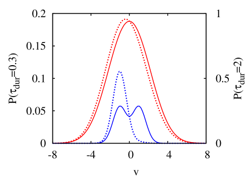
Figure 1: (color online) Quantum non-demolition setup: Two successive measurements. In each pair of the curves, the solid one gives the distribution of outcome of the first measurement while the dashed one gives the distribution for the second measurement provided the first measurement gave $v_{1}=-1$. Lower (upper) pair of curves corresponds to long, $\tau_{1,2}=2$ (short, $\tau_{1,2}=0.3$) duration of measurement. The long measurement is thus repeatable, the short one is not.

To illustrate the quantum aspect, let us set the initial density matrix to correspond to a pure state with the wave function that is an equal superposition of the base states $\pm$: $\hat{\rho}(0)=\hat{\sigma}_{1}$. We are interested in the average value of the corresponding pseudo-spin projection $\hat{\sigma}_{1}$ after the measurement provided the measurement gives the outcome $v$. We evaluate this average if we know the qubit density matrix $\hat{\rho}(v)$ conditioned on the outcome $v$,

$$\sigma_{1}(v)\equiv\mathrm{Tr}(\hat{\sigma}_{1}{\hat{\rho}}(v)).$$ (22)

As discussed in the previous Section, this qubit density matrix is computed from the normalized Fourier transform of $\hat{\rho}(\chi)$, the latter is obtained by solving Eqs. (20a) and (20b) on time interval $(0,\tau)$, $\tau$ being duration of the measurement.

Since Eqs. (20b) do contain the dephasing rate, the result will depend on actual depahsing. The answer reads

$$\sigma_{1}(v;\tau) = \frac{\cos(C_{12}v\tau)}{\cosh(v\tau)}e^{-\frac{C}{2}\tau}\,.$$ (23)

Here, we introduce dimensionless constants $C\equiv 4(S_{11}S_{22}-S_{12}^{2})/(\hbar a_{21})^{2}-1$ and $C_{12}=2S_{12}/\hbar a_{21}$. $C>0$ characterizes the quality of the detector, $C=0$ for a quantum-limited one. $C_{12}$ characterizes the correlations of the noises, for a quantum-limited detector $C_{12}=0$ as well.

Generally, $\sigma_{1}(v,\tau)$ quickly decays with increasing $\tau$. This manifests the dephasing of the superposition by the measurement. Remarkably enough, for a quantum-limited detector ($C=C_{12}=0$) and for a special value of the measurement outcome $v=0$ the dephasing is absent. The wave function retains its initial value for this particular value of output. This fact has been noted in the work Korotkov and termed ”quantum un-demolition measurement”. Let us note that the phase shift between the states $\pm$, acquired from the detector, $2\int_{0}^{\tau}\,dtQ(t)/\hbar$, is zero at this (rather improbable Korotkov ) value of the outcome. We stress that the strict correspondence between the phase shift and outcome does not hold for a general detector, so that $\sigma_{1}(v=0,\tau)=\exp(-C\tau/2)$ decreases with the measurement duration $\tau$ indicating the non-vanishing dephasing of the superposition. We plot $\sigma_{1}(v;\tau=1)$ versus the detector outcome $v$ for the duration of measurement $\tau=1$ in Fig. 2. The solid line is for the quantum-limited detector ($C=C_{12}=0$), and the dotted line is for the a worse detector ($C=C_{12}=1$).

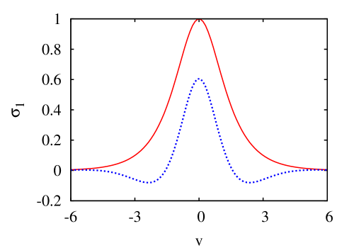
Figure 2: (color online) ”Un-demolition” measurement. The average value of pseudo-spin component $\sigma_{1}(v;\tau)$ conditioned on the detector outcome $v$ characterizes the dephasing of the superposition after a QND measurement of duration $\tau$($\tau=1$ for the plots). A quantum-limited detector ($C=C_{12}=0$, upper curve) allows for the quantum ”un-demolition” measurement ($\sigma_{1}=1$ at $v=0$). This does not work for a worse detector ($C=C_{12}=1$, lower curve).

IV The statistics of the CWLM of non-commuting variables

In the previous Section we provided simple examples to prove the use of the statistical approach. Thus encouraged, we turn to the statistics of the CWLM of non-commuting variables. The interaction Hamiltonian is now given by Eq. (16). We do not want to deal with the qubit Hamiltonian $H_{q}=\epsilon\sigma_{3}$ and shall assume that it is removed by transforming to the rotating frame. The same transform makes $\sigma_{1,2}$ to rotate with angular velocity $\epsilon/\hbar$. To compensate for this, let us presume that the signal from $\sigma_{1,2}$ is collected at frequencies $\epsilon/\hbar$ rather than at zero frequency as the signal from $\sigma_{3}$ is. Mathematically, we define the outcomes of the detectors $1,2$ as

$$\tau_{d}V_{1,2}=\int_{0}^{\tau_{d}}\,dt\bigl{[}\cos(\frac{\epsilon t}{\hbar})V_{1,2}(t)\mp\sin(\frac{\epsilon t}{\hbar})V_{2,1}(t)\bigr{]}\,.$$ (24)

This can be practically realized in a very same way as it is done in a radio set. One has to mix a high frequency signal with a reference signal of the same frequency and detect the low-frequency component of the product.

Let us evaluate $\hat{\rho}(\chi_{1},\chi_{2},\chi_{3})$. Without the term $H_{q}$, the Eq. (17) is readily solved in a proper basis in the pseudo-spin space. In this basis, one of the Pauli matrices is defined as $\hat{\sigma}_{\chi}=(\chi_{1}\hat{\sigma}_{1}+\chi_{2}\hat{\sigma}_{2}+\chi_{3}\hat{\sigma}_{3})/\chi_{s}$, while two others, $\hat{\sigma}_{\mu}$ and $\hat{\sigma}_{\nu}$, are chosen to be orthogonal to it. We have introduced $\chi_{s}$ as follows: $\chi_{s}\equiv\sqrt{\chi_{1}^{2}+\chi_{2}^{2}+\chi_{3}^{2}}$. We parameterize $\hat{\rho}$ as follows:

$$\hat{\rho}=\rho_{0}\hat{1}+\rho_{\chi}\hat{\sigma}_{\chi}+\rho_{\mu}\hat{\sigma}_{\mu}+\rho_{\nu}\hat{\sigma}_{\nu}\,.$$ (25)

From Eqs. (17) and (25) we obtain two equations involving $\rho_{0}$ and $\rho_{\chi}$:

$$\frac{\partial\rho_{0}}{\partial t} = ia_{21}\chi_{s}\rho_{\chi}-\frac{\chi_{s}^{2}}{2}S_{22}\rho_{0}\,,$$ (26a)

$$\frac{\partial\rho_{\chi}}{\partial t} = ia_{21}\chi_{s}\rho_{0}-(2\Gamma_{d}+\frac{\chi_{s}^{2}}{2}S_{22})\rho_{\chi}\,.$$ (26b)

We stress that the CWLM we are about to describe is hardly a measurement of the initial state of the qubit. In contrast to QND where the dephasing is limited to $1,2$ components, the input variables $\hat{Q}_{1,2,3}$ of the detectors randomly rotate the pseudo-spin in all three directions. The quantum information about initial state is lost rather quickly: at the time scale of $1/\Gamma_{d}$. That is, it is lost before a statistically reliable measurement result can be accumulated. This motivates us to choose the unpolarized density matrix as initial condition for the state of the qubit before the measurement,

$$\hat{\rho}(0)=\frac{1}{2}\hat{1}\,.$$ (27)

We will see however that despite the memory lost the CWLM of non-commutative variables can be rather informative.

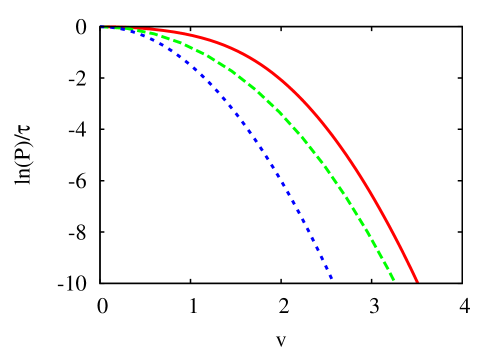
Figure 3: (color online) Logarithm of the outcome distribution. The curves from the top to the bottom: quantum-limited detector ($C_{d}=1/2$), worse detector ($C_{d}=2$), detector not connected to the qubit.

Let us first discuss the distribution of the detector outputs. We first solve Eqs. (26a) and (26b) with the initial condition (27), and then recall Eq. (5). In the limit of long durations $\tau\gg 1$, the log of the generating function reads:

$$-\log Z=\tau\left(C_{d}-\sqrt{C^{2}_{d}-\chi_{s}^{2}}+\frac{\chi_{s}^{2}}{2}\right)\,,$$ (28)

where $\chi_{i}$ has been made dimensionless $\chi_{i}S_{22}/a_{21}\to\chi_{i}$ as to give the cumulants of dimensionless outputs $v_{i}$. Here, $C_{d}\equiv\Gamma_{d}\tau_{m}=(C+1+C_{12}^{2})/2\geq 1/2$.

The cumulants of the outcomes can be evaluated by taking the derivatives of the $\log Z$ with respect to $\chi_{i}$. The presence of the qubit enhances output noises of each detector by the factor $1+1/C_{d}$:

$$\langle\langle v_{i}v_{j}\rangle\rangle = -\frac{\partial^{2}\log Z}{\partial\chi_{i}\partial\chi_{j}}|_{\chi_{i,j}=0}=\frac{1}{\tau}(1+\frac{1}{C_{d}})\delta_{ij}\,.$$ (29)

There is no correlation of noises between different detectors. Such correlation arise for fourth cumulants

$$\langle\langle v^{2}_{i}v^{2}_{j}\rangle\rangle=-\frac{\partial^{4}\log Z}{\partial\chi_{i}^{2}\partial\chi_{j}^{2}}|_{\chi_{i,j}=0}=-\frac{1+2\delta_{ij}}{(C_{d}\tau)^{3}}\,.$$ (30)

The distribution is isotropic in three outputs depending on $v\equiv\sqrt{v_{1}^{2}+v_{2}^{2}+v_{3}^{2}}$ only and in the limit of long durations we can calculate it by the saddle-point method, determining an optimal $\chi^{*}$ corresponding to a given outcome $v$. We obtain

$$\log P(v)=\log Z(\chi^{*}(v))\,;\,\,\,\frac{\partial\log Z}{\partial\chi_{s}}|_{\chi_{s}=\chi^{*}}=iv\tau\,.$$ (31)

$\chi^{*}$ is purely imaginary. We plot ${\log(P)}/\tau$ vs. $v$ for three different values of $C_{d}$ in Fig. 3. The solid line is for the quantum-limited detector ($C_{d}=1/2$), the dashed line is for the worse detector ($C_{d}=2$). The dotted line is for the detectors not connected to the qubit ($C_{d}=\infty$). So it is a parabola corresponding to the Gaussian distribution of outcomes in this case. We see that the distribution is concentrated at zero. Typical values of outcomes $v\sim 1/\sqrt{\tau}$ and for these typical values the distribution can be approximated estimated by a Gaussian one $P\sim\exp{(-v^{2}/2(1+1/C_{d}))}$. At larger (and thus atypical) values of outcomes ($v\simeq 1$) the distribution is essentially non-Gaussian. We see from the plots that the presence of the qubit exponentially enhances probabilities of such outcomes.

Let us discuss the correlation of the detector outputs and the pseudo-spin after such measurement thus turning to the joint statistics of the measurement outcomes and the resulting qubit state.

We characterize the correlation with a fidelity $f(v)$, inner product of the normalized vector of the outcomes and averaged pseudo-spin at given outcome $v$:

$$f=\frac{\sum_{i}\langle\sigma_{i}\rangle v_{i}}{v}\,;\,\,\,\,\langle\sigma_{i}\rangle=\mathrm{Tr}_{q}[\hat{\sigma}_{i}\hat{\rho}(v)]\,,$$ (32)

where $\hat{\rho}(v)$ is defined in Eq. (15) The fidelity is $1$ if the normalized values of the outputs precisely give all three pseudo-spin components. Analyzing the saddle-point solution for the $\hat{\rho}(v;\tau)$, we obtain that $f$ does not depend on $\tau$ in the limit $\tau\gg 1$. Importantly, at large values of the outcomes $v\gg 1$ the fidelity reaches the ideal value $f\approx 1-C_{d}/v$. This, quite unexpectedly, enables an efficient quantum monitoring of non-commuting variables.

The monitoring procedure is as follows. Starting from some initial state, one performs a series of repetitive measurements of duration $\tau$. The three outcomes $v_{i}$ of each measurement are written down. For most measurements, the values of the outcomes are typical, that is, do not exceed the results of such measurements correspond to low fidelity and are therefore discarded. One specifically waits for a measurement that gives sufficiently big values of outcomes. To decide if the outcomes are sufficiently big, one estimates the fidelity of each measurement given the values of outcomes and the relation $f(v)$. If one wants to achieve the desired accuracy $a_{des}$, one thus waits for the outcomes satisfying $f(v)>1-a_{des}$. The big values of outcomes guarantee that the fidelity $f(v)$ is sufficiently high. Sooner or later, a measurement gives the sufficiently big outcomes. The quantum monitoring takes place. At this moment, the state of the qubit is known with the accuracy desired and it is given by the values of outcomes $\hat{\rho}=\hat{\sigma_{i}}v_{i}/v$. Since $\hat{\rho}^{2}=\hat{1}$, this is a pure state.

We stress that the monitoring does not constitute a single-shot measurement of all components of the initial unknown quantum state. This would be forbidden by the basic laws of quantum mechanics. Indeed, the time required for an accurate monitoring exceeds by far the measurement time of the detectors. By this time, the initial state is completely forgotten. However, the monitoring gives the observer complete information about the final quantum state.

One also could argue that any pure state of the qubit can be obtained in a simpler fashion. One would just choose a proper $H_{q}$ and wait for dissipation to bring the qubit to the state of lowest energy. One could also try a projective measurement in a certain basis: after several tries, such measurement would give the state desired. We note however that for both approaches the resulting pure state is a priori known to the observer. This is not the case of quantum monitoring: here we let the quantum system to make ”its own choice” of the final pure state and do not enforce this choice by any means.

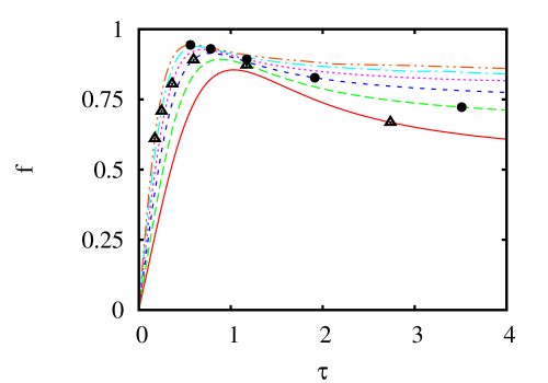
Figure 4: (color online) Fidelity of quantum monitoring $f$ vs. the measurement duration $\tau$ for quantum-limited detector. From upper to lower curve $v$ are respectively $4$, $3.5$, $3$, $2.5$, $2$, and $1.5$. Bullets at each curve indicate the value of $\tau$ at which the probability to get the outcome larger than the corresponding $v$ for each curve is $10\%$; triangles at each curve indicate the value of $\tau$ at which the probability to get the outcome larger than the corresponding $v$ for each curve is $50\%$.

The better the accuracy desired $a_{des}\equiv 1-f\ll 1$, the bigger outputs are required, $v>C_{d}/a_{des}$. The typical waiting time grows exponentially. To estimate it, we assume the duration of each measurement $\tau$ is in the order of $\tau_{m}$. This is because the longer durations are not favorable due to decoherence. The waiting time is inversely proportional to the probability to have sufficiently high outcomes $\tau_{w}\sim\tau/P(v;\tau)$. Since the success probability is exponentially small: $P(v;\tau)\sim\exp(-v^{2}\tau/2)$ from the saddle point solution, we then estimate $\tau_{w}\sim\exp(v^{2})$. Therefore, we shall expect

$$\mathrm{log}(\tau_{w})\sim a_{des}^{-2}.$$

This estimation of the waiting time of successful quantum monitoring sounds pessimistic or at least causes a doubt concerning the practical feasibility of the monitoring. To prove that the monitoring is practical, we are going to show that a reasonably high fidelity can be achieved in a reasonably short time.

The above arguments are based on the analytical saddle point solution valid at large $\tau$. Now we investigate the measurements of moderate duration, $\tau\sim 1$. This can only be done by numerical calculation. Solving Eqs. (26a) and (26b), and making the Fourier transformation according to Eq. (15), we evaluate and plot $f(v)$ of a single measurement of duration $\tau$ versus $\tau$ for the quantum-limited detector and the worse detector ($C_{d}=2$) in Fig. 4 and Fig. 5 respectively. Each curve gives $f(\tau)$ at a given outcome $v$. At each curve, we put a ”bullet” to indicate the duration of measurement $\tau$ at which the probability to obtain the outcomes larger than the given one is $10\%$. Similarly, we put a ”triangle” to indicate $\tau$ at which the probability is $50\%$. To find the positions of the symbols, for each $v$ we solve numerically for the values of $\tau$ that satisfy

$$\frac{\int_{v}^{+\infty}\mathrm{Tr}\hat{\rho}(v^{\prime},\tau)v^{\prime 2}dv^{\prime}}{\int_{0}^{+\infty}\mathrm{Tr}\hat{\rho}(v^{\prime},\tau)v^{\prime 2}dv^{\prime}}=10\%\,(50\%)$$ (33)

respectively. We see from the plots that $f=0.95$ is achieved for a quantum-limited detector at $v=4$ and $\tau=0.7$. At these parameters, $10\%$ of the measurements are successful, i.e. give the output $v>4$. To achieve a success, the measurement has to be repeated typically 10 times given the success probability of $10\%$. We conclude that the $5\%$ accuracy is typically achieved in a time interval $\simeq 10\times 0.7\tau_{m}=7\tau_{m}$. This is not much slower than the QND measurement of the same accuracy.

Let us explain the relation between the monitoring discussed and the quantum algorithms that use the results of partial measurement. These algorithms have been introduced in the context of two-qubit systems Bennett ; Deutsch but also may be applied to a general quantum state Nakazato . Speaking very generally, such algorithms start with a quantum state, pure or mixed, and aim at producing another state (pure and/or highly entangled). They proceed in steps. Each step involves interaction with ancilla qubits that results in an entanglement of the qubit and the ancillae. Importantly, the projective measurement of ancilla qubit(s) is performed at each step. The result of this measurement is used to decide upon next step: possible decisions include to re-request the initial state, to stop since the fidelity desired is reached, to apply a certain quantum gate.

The quantum monitoring proceeds similarly. It starts with an almost isotropic initial state: $\hat{\rho}=\hat{1}$. The qubit is being measured by our three independent quantum limit detectors during a time interval $\tau$. The outcome of the detectors is used to make a decision. If the sum of the square of the three detectors output $v_{i}$ of are small: $\sqrt{v_{1}^{2}+v_{2}^{2}+v_{3}^{2}}<4$, the measurement is disregarded: this is an analog of re-requesting the initial state. The measurement is repeated until the values of the outputs are sufficiently high $v=\sqrt{v_{1}^{2}+v_{2}^{2}+v_{3}^{2}}>4$. In this case, the monitoring may stop since its goal is reached: the qubit is purified to a state given by the detector outputs $v_{1}$, $v_{2}$ and $v_{3}$. Since the $v_{i}$ ($i=1,2,3$) are random, the purified state of the qubit is also random. Thus one could say that the CWLM monitoring implements a quantum algorithm of the sort described, in the same sense as an analogous computer may implement discrete computer algorithms.

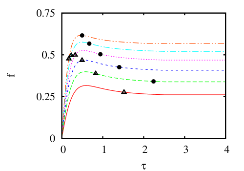
Figure 5: (color online) Fidelity of quantum monitoring $f$ versus the measurement duration $\tau$ for worse detector ($C_{d}=2$). From upper to lower curve $v$ are respectively $4$, $3.5$, $3$, $2.5$, $2$, and $1.5$. Bullets at each curve indicate the value of $\tau$ at which the probability to get the outcome larger than the corresponding $v$ for each curve is $10\%$; triangles at each curve indicate the value of $\tau$ at which the probability to get the outcome larger than the corresponding $v$ for each curve is $50\%$.

V Summary

In conclusion, we have shown how to evaluate the full statistics of the outcomes of a CWLM on a qubit. We are also able to evaluate joint probability distribution of the outcomes and the qubit variables after the measurement. For a single detector, we have illustrated the QND measurements and understood the recent proposal of quantum un-demolition measurement. Most interesting results concern the simultaneous CWLM of three non-commuting variables by three detectors. Such ”measurement” is obtrusive and typically scrambles the initial qubit wavefunction. However, we have demonstrated a high degree of correspondence between the wave function after the measurement and the outcomes of the three detectors. Therefore, such CWLM may be used for high-fidelity quantum monitoring of the qubit. The monitoring in fact amounts to a purification of the qubit state in a random direction $\vec{v}=(v_{1},v_{2},v_{3})/|v|$ at Bloch sphere, $v_{1-3}$ being random outputs of the detectors. We have drawn analogy with quantum algorithms that use the outputs of ancilla measurements to decide on the purification degree reached and the quantum gates to be applied.

The interpretation we give to the results is of course not the only possible one. The communications with several colleagues have convinced us that ”interesting” and ”important” defy an unambiguous definition as far as theory of quantum measurement is concerned. In any case, we have developed calculational tools to access the joint probability of the qubit degrees of freedom and the outcomes of linear detectors measuring the qubit. We have also derived the representative results. It is up to the reader to conclude.

Appendix A Derivation of the detector action

The derivation of the path-integral representation for a set of variables linear in boson creation/annihilation is a straightforward task. It is instrumental in dissipative quantum mechanics and therefore is to be found in basic literature on the subject. References Caldeira, are usually cited in this respect. Owing to the simplicity of the problem, there are many other derivations of the kind that are tailored to specific models (e.g. Kleinert ) and usually assume thermal equilibrium of the boson bath. To avoid any confusion, we present this part of the derivation here. We do the derivation in the most general terms possible and specify to the concrete model in use at the later stage of the calculation.

Let ${X}_{j}$ be a set of the variables linear in boson creation/annihilation operators, $\hat{X}_{j}(t)$ being the Heisenberg time-dependent operators of these variables. Let us first disregard the coupling with the qubit, so that the time dependence of $\hat{X}_{j}(t)$ is governed by the detector Hamiltonian $H_{d}$ only. Explicitly, the Heisenberg equation reads

$$\frac{d\hat{X}_{j}(t)}{dt}=\frac{i}{\hbar}[H_{d},\hat{X}_{j}(t)].$$

We are interested in the generating function of the variables which we present in the following form (c. f. Eq. 4)

$$Z(\{\chi_{j}(t)\})=\mathrm{Tr}\bigl{(}\overrightarrow{\mathrm{T}}e^{\frac{i}{2}\int dt\hat{X}_{j}(t)\chi_{j}(t)}\hat{\mathrm{\rho}_{d}}(0)\,\overleftarrow{\mathrm{T}}e^{\frac{i}{2}\int dt\hat{X}_{j}(t)\chi_{j}(t)}\bigr{)}\,.$$

We assume summation over repeating indexes $j$ and skip time indexes of $\hat{X}(t)$, $\chi(t)$ for brevity. Differentiating with respect to the parameters $\chi^{\pm}_{j}(t)$ of the generating function, one reproduces all possible products of the operators $\hat{X}_{j}(t)$.

Let us introduce a path integral over the variables $X^{\pm}_{j}(t)$ associated with the operators $\hat{X}_{j}(t)$ by means of the following identity:

$$Z(\{\chi_{j}(t)\})=\int\mathcal{D}{\bar{X}}^{+}\mathcal{D}{\bar{X}}^{-}{\rm Tr}\left[\overrightarrow{\mathrm{T}}\prod\limits_{t,j}\delta(X_{j}^{-}(t)-\hat{X}_{j}(t))e^{\frac{i}{2}\int dt({X}^{-}_{j}+{X}^{+}_{j})\chi_{j}}\hat{\mathrm{\rho}_{d}}(0)\right.$$

$$\left.\overleftarrow{\mathrm{T}}\prod\limits_{t,j}\delta(X_{j}^{+}(t)-\hat{X}_{j}(t))\right]\,.$$ (34)

Here we insert $\delta$-functions that replace the operators $\hat{X}_{j}(t)$ by the fluctuating fields $X_{j}^{\pm}(t)$, separately for two parts of the Keldysh contour.

The use of this representation is that we can treat the coupling between the detector and an arbitrary quantum system in the form of the influence functional. If the coupling between the detector and the system has the form

$$H_{int}=\sum_{j}\hat{X}_{j}(t)\hat{S}_{j};$$

$\hat{S}_{j}$ being operators defined in the subspace of the quantum system, we can formally substitute $\hat{X}_{j}(t)\to{X}^{\pm}_{j}(t)$. The resulting influence functional thus reads

$${\cal Z}_{Iq}(\{X^{-}_{j}(t)\},\{X^{+}_{j}(t)\})=\mathop{{\rm Tr}}\limits_{S}\bigl{(}\overrightarrow{\mathrm{T}}e^{-\frac{i}{\hbar}\int dt{X}^{-}_{j}\hat{S}_{j}}\hat{\mathrm{\rho}_{S}}(0)\,\overleftarrow{\mathrm{T}}e^{\frac{i}{\hbar}\int dt{X}^{+}_{j}\hat{S}_{j}}\bigr{)}\,,$$ (35)

where the trace is over the subspace of the quantum system, $\hat{\mathrm{\rho}_{S}}(0)$ is its initial density matrix and the time dependence of $\hat{S}_{j}$ is governed by the separate Hamiltonian on the subspace of the quantum system.

Let us turn to the evaluation of the representation (34). To facilitate the operations with $\delta$-functions, we represent them by means of extra integration over the auxiliary variables $k^{\pm}(t)/\hbar$. At each time moment,

$$\delta(X_{j}^{\pm}-\hat{X}_{j})=\int\frac{dk_{j}^{\pm}}{2\pi}e^{ik_{j}^{+}(X_{j}^{\pm}-\hat{X}_{j})}.$$

With these extra variables, the integral becomes

$$Z(\{\chi_{j}(t)\})=\int\mathcal{D}{\bar{X}}^{+}\mathcal{D}{\bar{X}}^{-}\mathcal{D}{\bar{k}}^{+}\mathcal{D}{\bar{k}}^{-}e^{{i}\int dt{X}^{-}_{j}(k^{-}_{j}+\chi_{j}/2)}e^{{i}\int dt{X}^{+}_{j}(k^{+}_{j}+\chi_{j}/2)}$$

$${\rm Tr}\left[\overrightarrow{\mathrm{T}}e^{-{i}\int dt{\hat{X}}_{j}k_{j}^{-}}\hat{\mathrm{\rho}_{d}}(0)\overleftarrow{\mathrm{T}}e^{-{i}\int dt{\hat{X}}_{j}k_{j}^{+}}\right].$$ (36)

Let us now take the trace over the boson degrees of freedom. To do this, we use the widely known relation

$$\langle e^{\hat{A}}e^{\hat{B}}\rangle=e^{\langle\frac{{\hat{A}^{2}+\hat{B}^{2}}}{2}+\hat{A}{\hat{B}}\rangle}$$

that holds for $\hat{A},\hat{B}$ that are linear in boson operators under condition of Wick’s theorem. This allows us to express the trace in terms of the two-point correlators of boson variables, $\langle\hat{X}_{i}(t)\hat{X}_{j}(t^{\prime})\rangle$. We may assume $\langle\hat{X}_{j}\rangle\equiv 0$ without compromising generality. The resulting expression reads

$$Z(\{\chi_{j}(t)\})=\int\mathcal{D}{\bar{X}}^{+}\mathcal{D}{\bar{X}}^{-}\mathcal{D}{\bar{k}}^{+}\mathcal{D}{\bar{k}}^{-}e^{{i}\int dt{X}^{-}_{j}(k^{-}_{j}+\chi_{j}/2)}e^{{i}\int dt{X}^{+}_{j}(k^{+}_{j}+\chi_{j}/2)}e^{\tilde{A}_{d}};$$

$$\tilde{A}_{d}=-\int dtdt^{\prime}\left[\frac{1}{2}k^{+}_{i}(t)k^{+}_{j}(t^{\prime})\langle\overleftarrow{\mathrm{T}}(\hat{X}_{i}(t)\hat{X}_{j}(t^{\prime}))\rangle+\frac{1}{2}k^{-}_{i}(t)k^{-}_{j}(t^{\prime})\langle\overrightarrow{\mathrm{T}}(\hat{X}_{i}(t)\hat{X}_{j}(t^{\prime}))\rangle\right.$$

$$\left.+k^{-}_{i}(t)k^{+}_{j}(t^{\prime})\langle\hat{X}_{i}(t)\hat{X}_{j}(t^{\prime})\rangle\right].$$ (37)

It is instructive to introduce at this stage ”classical” and ”quantum” variables defining $X^{\pm}_{j}=X_{j}\pm\hbar x_{j}/2$, $k^{\pm}_{j}=K_{j}\pm k_{j}/2\hbar$. In these variables, the two-point correlators are naturally collected to symmetrized noises $S_{ij}(t,t^{\prime})$ and Kubo-like response functions $A_{ij}(t,t^{\prime})$,

$$S_{ij}(t,t^{\prime})=\frac{1}{2}\langle\hat{X}_{i}(t)\hat{X}_{j}(t^{\prime})+\hat{X}_{j}(t^{\prime})\hat{X}_{i}(t)\rangle;\;A_{ij}(t,t^{\prime})=-\frac{i}{\hbar}\Theta(t-t^{\prime})\langle[\hat{X}_{i}(t),\hat{X}_{j}(t^{\prime})]\rangle.$$

and the action becomes

$$\tilde{A}_{d}=-\int dtdt^{\prime}\left[2K_{i}(t)K_{j}(t^{\prime})S_{ij}(t,t^{\prime})+{i}k_{i}(t)K_{j}(t^{\prime})A_{ij}(t,t^{\prime})\right].$$

and does not contain $\hbar$. One can now integrate over the auxiliary variables $K_{j}(t),k_{j}(t)$ to get the action in terms of $X_{j}(t),x_{j}(t)$. This Gaussian integral can be readily taken by the saddle-point method. For our model, it is convenient to make the time-local approximation first. We replace the kernels $S_{ij},A_{ij}$ with their time-local expressions Eqs.(7, 8) and perform integration over $K,k$ to arrive at Eq. 9.

Appendix B Augmented Bloch-Redfield equation and Lindblad form

In this appendix we cast the Eq. (13) to the Lindblad formLindblad to illustrate the entanglement of the qubit and detector and to prove the positivity of the density matrix encompassing the qubit and output variable of the detector.

To specify this underlying density matrix, it is useful to introduce a quantum variable $\hat{p}$ defined as

$$\hat{p}=\int_{0}^{t}\hat{V}(t^{\prime})\,dt^{\prime}\,.$$

This variable represents the integrated detector output over the interval $(0,t)$. It differs only by a factor $t$ from the outcome $V_{o}$ of the measurement at the same time interval $(0,t)$ as we have defined in the main text.

We denote by $p$ and $|p\rangle$ the eigenvalue and eigenvector of $\hat{p}$ respectively: $\hat{p}|p\rangle=p|p\rangle$. The subject of our interest is the time-dependent reduced density matrix in the space $|\mathrm{spin}\rangle\bigotimes|p\rangle$, $\hat{\rho}(p,p^{\prime};t)$, where ”hat” denotes the matrix in the pseudo-spin space. Since $p$ is related to $V_{o}$ upon a factor, this matrix is equivalent to $\hat{R}(V_{o},V^{\prime}_{o})$ used in the main text. The quantity $\hat{\rho}(\chi)$ in the augmented Bloch-Redfield equation is related to the diagonal part of this density matrix by Fourier transform

$$\hat{\rho}(p,p;t)=\int d\chi e^{-ip\chi}\hat{\rho}(\chi,t)\,.$$ (38)

Making the inverse Fourier transform, we deduce from Eqs. (13) and (38) the equation for $\hat{\rho}(p,p;t)$:

$$\frac{\partial{\hat{\rho}}(p,p;t)}{\partial t} = -\frac{i}{\hbar}[H_{q},\hat{\rho}(p,p;t)]+\frac{S_{22}}{2}\frac{\partial^{2}\hat{\rho}(p,p;t)}{\partial p^{2}}$$ (39)

$$-\frac{a_{21}}{2}\bigl{(}\frac{\partial\hat{\rho}(p,p;t)}{\partial p}\hat{\sigma}_{3}+\hat{\sigma}_{3}\frac{\partial\hat{\rho}(p,p;t)}{\partial p}\bigr{)}$$

$$-\frac{iS_{12}}{\hbar}\bigl{(}\frac{\partial\hat{\rho}(p,p;t)}{\partial p}\hat{\sigma}_{3}-\hat{\sigma}_{3}\frac{\partial\hat{\rho}(p,p;t)}{\partial p}\bigr{)}$$

$$-\frac{S_{11}}{\hbar^{2}}\bigl{(}\hat{\rho}(p,p;t)-\hat{\sigma}_{3}\hat{\rho}(p,p;t)\hat{\sigma}_{3}\bigr{)}\,.$$

This is an evolution equation in partial derivatives.

Next, we demonstrate that Eq. (39) is indeed of a Lindblad type. This also proves that the density matrix satisfying the equation has positive diagonal elements. We work in the space $|\mathrm{spin}\rangle\bigotimes|p\rangle$. We can check that the operator $\hat{o}=i\frac{\partial}{\partial p}$ has the following properties:

$$\langle p|\hat{\rho}\hat{o}|p^{\prime}\rangle = -i\frac{\partial\hat{\rho}(p,p^{\prime};t)}{\partial p^{\prime}}\,,$$ (40a)

$$\langle p|\hat{o}\hat{\rho}|p^{\prime}\rangle = i\frac{\partial\hat{\rho}(p,p^{\prime};t)}{\partial p}\,.$$ (40b)

The Lindblad form of an evolution equation readsLindblad ; Presilla

$$\frac{\partial\hat{\rho}}{\partial t}=-\frac{i}{\hbar}\bigl{[}H,\hat{\rho}\bigr{]}+\frac{1}{2}\sum_{\nu}\bigl{(}[\hat{L}_{\nu}\hat{\rho},\hat{L}_{\nu}^{{\dagger}}]+[\hat{L}_{\nu},\hat{\rho}\hat{L}_{\nu}^{{\dagger}}]\bigr{)}\,,$$ (41)

where $H$ is a Hermitian operator, generally not coinciding with the qubit Hamiltonian, and $\hat{L}_{\nu}$ ($\nu=1,\cdots$) are arbitrary operators. We need to prove that a proper choice of the Lindblad operators $\hat{L}_{\nu}$ and the Hamiltonian $H$ reproduces Eq. 39.

To do so, we introduce $2$ Lindblad operators as follows:

$$\hat{L}_{1} = \sqrt{\frac{4S_{11}S_{22}-4S_{12}^{2}-\hbar^{2}a_{21}^{2}}{4\hbar^{2}S_{22}}}\,\hat{\sigma}_{3}\,,$$ (42a)

$$\hat{L}_{2} = \sqrt{S_{22}}\bigl{(}\hat{o}-\frac{S_{12}}{\hbar S_{22}}\hat{\sigma}_{3}-\frac{ia_{21}}{2S_{22}}\hat{\sigma}_{3}\bigr{)}\,,$$ (42b)

here $4S_{11}S_{22}-4S_{12}^{2}-\hbar^{2}a_{21}^{2}\geq 0$ is guaranteed by the Cauchy-Schwartz inequality (see Sec. II). The Hermitian operator reads:

$$H=H_{q}-\frac{\hbar a_{21}}{2}\hat{o}\hat{\sigma}_{3}\,.$$ (43)

where $H_{q}$ is the qubit Hamiltonian. We substitute the operators to Eq. (41) to obtain the following:

$$\frac{\partial\hat{\rho}(p,p^{\prime};t)}{\partial t} = -\frac{i}{\hbar}\bigl{[}H,\hat{\rho}(p,p^{\prime};t)\bigr{]}$$ (44)

$$+\frac{S_{22}}{2}\bigl{(}2\frac{\partial^{2}\hat{\rho}(p,p^{\prime};t)}{\partial p\partial p^{\prime}}+\frac{\partial^{2}\hat{\rho}(p,p^{\prime};t)}{\partial p^{2}}+\frac{\partial^{2}\hat{\rho}(p,p^{\prime};t)}{\partial p^{\prime 2}}\bigr{)}$$

$$-\frac{a_{21}}{2}\bigl{(}\frac{\partial\hat{\rho}(p,p^{\prime};t)}{\partial p^{\prime}}\hat{\sigma}_{3}+\frac{\partial\hat{\rho}(p,p^{\prime};t)}{\partial p}\hat{\sigma}_{3}+\hat{\sigma}_{3}\frac{\partial\hat{\rho}(p,p^{\prime};t)}{\partial p}+\hat{\sigma}_{3}\frac{\partial\hat{\rho}(p,p^{\prime};t)}{\partial p^{\prime}}\bigr{)}$$

$$-\frac{iS_{12}}{\hbar}\bigl{(}\frac{\partial\hat{\rho}(p,p^{\prime};t)}{\partial p}\hat{\sigma}_{3}+\frac{\partial\hat{\rho}(p,p^{\prime};t)}{\partial p^{\prime}}\hat{\sigma}_{3}-\hat{\sigma}_{3}\frac{\partial\hat{\rho}(p,p^{\prime};t)}{\partial p}-\hat{\sigma}_{3}\frac{\partial\hat{\rho}(p,p^{\prime};t)}{\partial p^{\prime}}\bigr{)}$$

$$+\frac{S_{11}}{\hbar^{2}}\bigl{(}\hat{\sigma}_{3}\hat{\rho}(p,p^{\prime};t)\hat{\sigma}_{3}-\hat{\rho}(p,p^{\prime};t)\bigr{)}\,.$$

We made use of the properties (40a) and (40b). We have not done yet, since the above equation is for a two-indexed density matrix $\hat{\rho}(p,p^{\prime})$ and not for its diagonal part. We still have to prove that the above equation does not mix the diagonal and non-diagonal elements. So that, to relate Eq. (39) with Eq. (44), we change variables as follows:

$$P_{s} = \frac{p+p^{\prime}}{2}\,,$$ (45a)

$$P_{d} = \frac{p-p^{\prime}}{2}\,.$$ (45b)

Thus,

$$\frac{\partial}{\partial p} = \frac{1}{2}(\frac{\partial}{\partial P_{s}}+\frac{\partial}{\partial P_{d}})\,,$$ (46a)

$$\frac{\partial}{\partial p^{\prime}} = \frac{1}{2}(\frac{\partial}{\partial P_{s}}-\frac{\partial}{\partial P_{d}})\,.$$ (46b)

From Eqs. (44), (46a) and (46b) we obtain:

$$\frac{\partial\hat{\rho}(P_{s},P_{d};t)}{\partial t} = -\frac{i}{\hbar}\bigl{[}H,\hat{\rho}(P_{s},P_{d};t)\bigr{]}+\frac{S_{22}}{2}\frac{\partial^{2}\hat{\rho}(P_{s},P_{d};t)}{\partial P_{s}^{2}}$$ (47)

$$-\frac{a_{21}}{2}\bigl{(}\frac{\partial\hat{\rho}(P_{s},P_{d};t)}{\partial P_{s}}\hat{\sigma}_{3}+\hat{\sigma}_{3}\frac{\partial\hat{\rho}(P_{s},P_{d};t)}{\partial P_{s}}\bigr{)}$$

$$-\frac{iS_{12}}{\hbar}(\frac{\partial\hat{\rho}(P_{s},P_{d};t)}{\partial P_{s}}\hat{\sigma}_{3}-\hat{\sigma}_{3}\frac{\partial\hat{\rho}(P_{s},P_{d};t)}{\partial P_{s}})$$

$$+\frac{S_{11}}{\hbar^{2}}\hat{\sigma}_{3}\hat{\rho}(P_{s},P_{d};t)\hat{\sigma}_{3}\,.$$

Eqs. (39) and (47) has the same form. Therefore, we have proved that $\hat{\rho}(p,p;t)$ satisfies the Lindblad equation in the $|\mathrm{spin}\rangle\bigotimes|p\rangle$ space matrix form and thus is positive.

We can straightforwardly extend the above scheme to Eq. (17) of Sec. II that is valid for the case of three detectors. In this case, we introduce $6$ Lindblad operators

$$\hat{L}_{1i} = \sqrt{\frac{4S_{11}S_{22}-4S_{12}^{2}-\hbar^{2}a_{21}^{2}}{4\hbar^{2}S_{22}}}\,\hat{\sigma}_{i}\,,$$ (48a)

$$\hat{L}_{2i} = \sqrt{S_{22}}\bigl{(}\hat{o}_{i}-\frac{S_{12}}{\hbar S_{22}}\hat{\sigma}_{i}-\frac{ia_{21}}{2S_{22}}\hat{\sigma}_{i}\bigr{)}\,,$$ (48b)

where $i=1,2,3$. The Hermitian operator reads:

$$H=H_{q}-\frac{\hbar a_{21}}{2}\sum_{i=1}^{3}\hat{o}_{i}\,,$$ (49)

where $\hat{o}_{i}=i\frac{\partial}{\partial p_{i}}$ and $p_{i}$ are the eigenvalues of the operator $\hat{p}_{i}=\int_{0}^{t}\hat{V}_{i}(t^{\prime})\,dt^{\prime}$ ($i=1,2,3$) corresponding to each detector.

To conclude, we have shown that the density matrix $\hat{\rho}(p,p^{\prime};t)$ in the space $|\mathrm{spin}\rangle\bigotimes|p\rangle$ satisfies the Lindblad equation and thus its diagonal part is positive. The diagonal part of the matrix is related to the quantity $\hat{\rho}(\chi,t)$ in the Sec. II by the Fourier transform. We note that Lindblad operators Eqs. (42a, 42b, 48a, 48b) include both the degree of qubit and the degree of the detector(s). This signals the entanglement of the qubit and detector(s) In this sense, we measure both the qubit and detector(s) in the context of FCS theory.

References

- (1) V. B. Braginsky and F. Y. Khalili, Quantum Measurement (Cambridge University Press, Cambridge, 1992).
- (2) A. J. Leggett, Science 307, 871 (2005).
- (3) V. Cerletti, W. A. Coish, O. Gywat, D. Loss, Nanotechnology 16, R27 (2005).
- (4) G. Wendin and V. Shumeiko, in Handbook of Theoretical and Computational Nanotechnology, edited by M. Riech and W. Schommers (ASP, Los Angeles, 2006).
- (5) M. A. Nielsen and I. L. Chuang, Quantum Computations and Quantum Information (Cambridge University Press, Cambridge, 2000).
- (6) A. N. Korotkov, Phys. Rev. B 60, 5737 (1999).
- (7) D. V. Averin, in Quantum Noise in Mesoscopic Physics, edited by Yu.V. Nazarov (Kluwer, Dordrecht, 2003).
- (8) A. A. Clerk, S. M. Girvin and A. D. Stone, Phys. Rev. B 67, 165324 (2003).
- (9) A. N. Jordan and M. Büttiker, Phys. Rev. Lett. 95, 220401 (2005).
- (10) A. N. Korotkov and A. N. Jordan, Phys. Rev. Lett. 97, 166805 (2006).
- (11) D. V. Averin, in ”Exploring the quantum/classical frontier: recent advances in macroscopic quantum phenomena”, Ed. by J. R. Frieman and S. Han, (Nova Publishes, Hauppauge, NY, 2002), p441.
- (12) S. A. Gurvitz, Phys. Rev. B 56, 15215 (1997).
- (13) A. B. Zorin Phys. Rev. Lett. 76, 4408 (1996).
- (14) S. Pilgram and M. Büttiker, Phys. Rev. Lett. 89, 200401 (2002).
- (15) D. V. Averin, K. Rabenstein and V. K. Semenov, Phys. Rev. B 73, 094504 (2006).
- (16) A. Fedorov, A. Shnirman, G. Schön and A. Kidiyarova-Shevchenko, Phys. Rev. B 75, 224504 (2007).
- (17) N. Gisin, G. Ribordy, W. Tittel and H. Zbinden, Rev. Mod. Phys. 74, 145 (2002).
- (18) P. Busch , T. Heinonen, and P. Lahti, Phys. Rep. 452, 155 (2007).
- (19) A. Di Lorenzo, G. Campagnano and Yu. V. Nazarov, Phys. Rev. B 73, 125311 (2006).
- (20) L. S. Levitov and G. B. Lesovik, JETP Lett. 55, 555 (1992). L. S. Levitov and G. B. Lesovik, JETP Lett. 58, 230 (1993). L. S. Levitov, H. Lee and G. B. Lesovik, J. Math. Phys. (N.Y.) 37, 4845 (1996).
- (21) Yu. V. Nazarov, Ann. Phys. (Leipzig) 8, Spec. Issue SI-193, 507 (1999).
- (22) Y. Makhlin, G. Schön and A. Shnirman, Phys. Rev. Lett. 85, 4578, (2000); G. B. Lesovik, F. Hassler and G. Blatter, Phys. Rev. Lett. 96, 106801 (2006).
- (23) V. B. Braginsky and F. Y. Khalili, Rev. Mod. Phys. 68, 1 (1996).
- (24) A. O. Caldeira and A. J. Leggett, Ann. Phys. 149, 374 (1983); A. O. Caldeira and A. J. Leggett, Physica A 121, 587 (1983).
- (25) R. P. Feynman and F. L. Vernon, Ann. Phys. (N.Y.) 24, 118, (1963).
- (26) L. V. Keldysh, Zh. Eksp. Teor. Fiz. 47, 1515 (1964); [Soviet Phys. JETP 20, 1018 (1965)].
- (27) J. Rammer and H. Smith, Rev. Mod. Phys. 58 323 (1986).
- (28) Yu. V. Nazarov, M. Kindermann, Eur. Phys. J. B. 35 413, 2003.
- (29) M. Kindermann, Yu. V. Nazarov and C. W. J. Beenakker, Phys. Rev. B 69, 035336, (2004), appendix A.
- (30) Y. Makhlin, G. Schön and A. Shnirman, Rev. Mod. Phys. 73 357, (2001).
- (31) H. Kleinert, Path Integrals in Quantum Mechanics, Statistics, Polymer Physics and Financial Markets, World Scientific (Singapore), 3rd edition, 2005.
- (32) A. Romito and Yu.V. Nazarov, Phys. Rev. B 70, 212509 (2004).
- (33) G. Lindblad, Comm. Math. Phys. 48, 119 (1976).
- (34) C. Presilla, R. Onofrio, U. Tambini, Ann. Phys. 248, 95 (1996).
- (35) A. Lupascu, S. Saito, T. Picot, P. C. de Groot, C. J. P. M. Harmans and J. E. Mooij, Nat. Phys. 3, 119 (2007).
- (36) C. H. Bennett, G. Brassard, S. Popescu, B. Schumacher, J. A. Smolin and W. K. Wootters, Phys. Rev. Lett. 76, 722 (1996).
- (37) D. Deutsch, A. Ekert, R. Jozsa, C. Macchiavello, S. Popescu and A. Sanpera, Phys. Rev. Lett. 77, 2818 (1996).
- (38) H. Nakazato, T. Takazawa and K. Yuasa, Phys. Rev. Lett. 90, 060401 (2003).