Low-temperature thermodynamics for a flat-band ferromagnet: Rigorous versus numerical results

Abstract

The repulsive Hubbard model on a sawtooth chain exhibits a lowest single-electron band which is completely dispersionless (flat) for a specific choice of the hopping parameters. We construct exact many-electron ground states for electron fillings up to 1/4. We map the low-energy degrees of freedom of the electron model to a model of classical hard dimers on a chain and, as a result, obtain the ground-state degeneracy as well as closed-form expressions for the low-temperature thermodynamic quantities around a particular value of the chemical potential. We compare our analytical findings with complementary numerical data. Although we consider a specific model, we believe that some of our results such as a low-temperature peak in the specific heat are generic for flat-band ferromagnets.

Introduction and motivation. The Hubbard model is the simplest model for strongly interacting electrons in a solid.thehubbard Nevertheless, the analysis of its properties is a difficult task. Only relatively few rigorous results are known, see e.g. Refs. thehubbard, ; lieb, ; tasaki_jpcm, . A special focus of rigorous studies is the search for ground state (GS) ferromagnetism (FM). vollhardt ; mielke ; tasaki ; tasaki_ptp In particular, different (nonbipartite) lattices supporting dispersionless (flat) single-electron bands were studied in some detail. The Hubbard model on such lattices may have ferromagnetic GS’s for certain electron concentrations (so-called flat-band FM).mielke ; tasaki ; tasaki_ptp An important aspect of these studies is the existence of eigenstates where electrons are localized on finite areas of the lattice. Recently, the concept of flat-band FM has been developed further, see e.g. Refs. ichimura, ; tanaka, ; sekizawa, ; nishino, ; tanaka_tasaki, , and relations to materials with (almost) flat bands have been pointed out. Another recent development is the discovery of a class of exact eigenstates for antiferromagnetic spin models on certain frustrated lattices. lm1 These states, called localized-magnon states, are GS’s of the $XXZ$ Heisenberg antiferromagnet (AFM) in strong magnetic fields, and lead to interesting low-temperature physics near the saturation field such as a macroscopic magnetization jump,lm1 a field-tuned lattice instability,lm5 a finite residual entropy,lm6a ; lm6 ; lm7 an enhanced magnetocaloric effect,lm6a or a finite-temperature order-disorder phase transition in 2D Heisenberg spin systems. lm7 On the one-particle level the localized eigenstates of the electronic system and the spin system are identical.honecker_richter However, for multi-particle states the different statistics and types of interaction clearly become relevant.

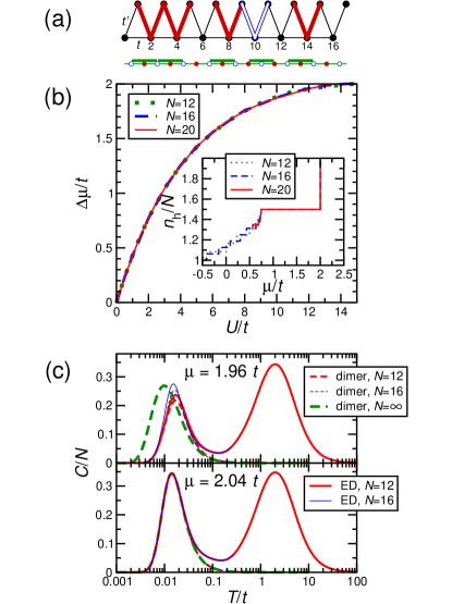
Figure 1: (Color online) (a) Sawtooth lattice with auxiliary lattice for dimer mapping indicated below. Each electron state localized in a valley of the sawtooth lattice corresponds to a dimer on a site of the auxiliary lattice. Filled (open) symbols denote spin-up (spin-down) electrons. The presence of a dimer on a site of the auxiliary lattice excludes the presence of dimers on the two adjacent sites. (b) Main panel: Charge gap $\Delta\mu=E(N/2+1)-2\,E(N/2)+E(N/2-1)$ at quarter filling versus $U$. Inset: Hole concentration $n_{\rm h}/N=2-n/N$ versus chemical potential $\mu$ for $U=4\,t$. (c) Specific heat $C$ per site $N$. ED results are for $U=4\,t$. Note that for $\mu=2.04\,t$ different system sizes are indistinguishable.

In the present Rapid Communication we apply the ideas elaborated for frustrated AFM’s having localized-magnon GS’s to the Hubbard model with a flat band. We focus on the sawtooth chain shown in Fig. 1a and characterize the complete manifold of highly degenerate GS’s for electron concentrations up to quarter filling. Using a grand-canonical description and a mapping to a classical hard-dimer problem, we derive explicit analytical expressions for the GS jump of the electron concentration, the residual entropy at a particular value of the chemical potential $\mu_{0}$, and the contribution of the GS manifold to thermodynamic quantities such as the specific heat. We believe that the Hubbard model on other highly frustrated lattices shows universal behavior as it has been demonstrated for spin systems.lm6 ; lm7 Therefore, we expect that similar considerations can be performed for other lattices with flat bands, too.

The sawtooth-chain Hubbard model attracts much attention since the 90s and was discussed earlier within different approaches.penc Moreover, a number of compounds are known to be described by the sawtooth-chain Heisenbergsawtooth or periodic Andersonpam models.

We consider the $N$-site Hubbard Hamiltonian

$$H = \sum_{\sigma=\uparrow,\downarrow}H_{0\sigma}+H_{U}\,,\quad H_{U}=U\sum_{i}n_{i,\uparrow}n_{i,\downarrow}\,,$$

$$H_{0\sigma} = \sum_{\langle i,j\rangle}t_{i,j}\left(c_{i,\sigma}^{\dagger}c_{j,\sigma}+c_{j,\sigma}^{\dagger}c_{i,\sigma}\right)+\mu\sum_{i}n_{i,\sigma}\,,$$ (1)

where $i$ denotes the lattice sites (see Fig. 1a), $\langle i,j\rangle$ denote pairs of nearest neighbors, the $c_{i,\sigma}^{\dagger}$ ($c_{i,\sigma}$) are the usual fermion operators, $n_{i,\sigma}=c_{i,\sigma}^{\dagger}c_{i,\sigma}$, and periodic boundary conditions are implied. We choose the relation $t^{\prime}=\sqrt{2}\,t>0$ between the hopping along the zig-zag path $t^{\prime}$ and the hopping along the base line $t$ in order to render the lowest single-electron band completely flat (see e.g. Refs. tasaki, ; tasaki_ptp, ; honecker_richter, ). $U\geq 0$ is the on-site Coulomb repulsion and $\mu$ is the chemical potential. The sawtooth Hubbard model (1) is a particular case of Tasaki’s model for which the GS exhibits saturated FM for a half-filled flat band, i.e. when the number of electrons is $n=N/2$.tasaki ; tasaki_ptp

Localized-electron states. Eigenstates which do not feel $U>0$. Localized-electron states are a standard tool in the field of flat-band FM (see, e.g., Refs. mielke, ; tasaki, ; tasaki_ptp, ; ichimura, ; nishino, ). As a basis for further discussion, we review the construction for the sawtooth chain in a formulation inspired by localized magnons in highly frustrated AFM’s lm1 (see also Ref. honecker_richter, ). Since the lowest single-electron band is completely flat, it is possible to localize the corresponding states in real space, namely on the three consecutive sites forming a ‘valley’ on the sawtooth chain. Let us introduce the operators $l_{2j,\sigma}^{\dagger}=c_{2j-1,\sigma}^{\dagger}-\sqrt{2}\,c_{2j,\sigma}^{\dagger}+c_{2j+1,\sigma}^{\dagger}$ which satisfy $[H_{0\sigma},l^{\dagger}_{2j,\sigma}]_{-}=\varepsilon_{-}\,l^{\dagger}_{2j,\sigma}$ where $\varepsilon_{-}=-2\,t+\mu$ is the energy of the flat band. Then the complete set of $N$ single-electron states belonging to the flat band can be written as $l_{2j,\sigma}^{\dagger}|0\rangle$ with $|0\rangle$ denoting the vacuum state. Application of $n$ distinct operators $l_{2j,\sigma}^{\dagger}$ to $|0\rangle$ yields $n$-electron states. If the valleys belonging to the $l_{2j,\sigma}^{\dagger}$ with different spin are disconnected these are exact eigenstates of the full Hamiltonian with energy $E_{n}=n\,\varepsilon_{-}$. However, these simple product states do not exhaust the exact $n$-electron eigenstates with energy $E_{n}$.

To construct all $n$-electron states with $U$-independent energy $E_{n}=n\,\varepsilon_{-}$ systematically we proceed as follows. We start with a fully spin-up-polarized state $l_{2j,\uparrow}^{\dagger}l_{2(j+1),\uparrow}^{\dagger}\ldots l_{2(j+L-1),\uparrow}^{\dagger}|0\rangle$, i.e. localized electrons occupying a cluster of $L$ consecutive valleys. Now we exploit the $SU(2)$-invariance of the model (1) to construct new eigenstates by acting with $S^{-}=\sum_{i}c_{i,\downarrow}^{\dagger}c_{i,\uparrow}$ on this state and using the relations $[S^{-},l_{2j,\uparrow}^{\dagger}]_{-}=l_{2j,\downarrow}^{\dagger}$ and $[S^{-},l_{2j,\downarrow}^{\dagger}]_{-}=0$. $L$-fold application of $S^{-}$ yields the fully spin-down-polarized state $l_{2j,\downarrow}^{\dagger}l_{2(j+1),\downarrow}^{\dagger}\ldots l_{2(j+L-1),\downarrow}^{\dagger}|0\rangle$. However, the action of $(S^{-})^{m},\;m=1,\ldots,L-1,$ yields $L-1$ further eigenstates with the same energy $L\,\varepsilon_{-}$ which cannot be expressed by applying only one product of $l_{2j,\sigma}^{\dagger}$ operators on $|0\rangle$ but rather are given by linear combinations. Evidently, the same states are obtained if we use $S_{{\rm cluster},L}^{-}=\sum_{i=2j-1}^{2(j+L)-1}c_{i,\downarrow}^{\dagger}c_{i,\uparrow}$ instead of $S^{-}$. Finally, we can use these cluster states as building blocks for product states containing more than one cluster of occupied valleys. As long as individual clusters are separated by empty valleys, such product states remain exact eigenstates. All these states are eigenstates of $H$ and have a definite value of total $S^{z}$, but they do not necessarily carry a definite total spin $S$.

Let us discuss some further important properties of the above constructed exact $n$-electron eigenstates with $n\leq N/2$. Firstly, they are GS’s for $U=0$. Note that their energy $E_{n}=n\,\varepsilon_{-}$ is independent of $U$. Since $H_{U}$ is a positive semidefinite operator for $U>0$ the on-site $H_{U}$ can only increase energies. Thus, the localized-electron states remain GS’s for $U>0$. Secondly, the localized $n$-electron states are linearly independent, which is connected with the fact (as in the case of spin systems, see Ref. schmidt, ) that the middle site is unique to each valley. Finally, we have to discuss whether these states are the only GS’s. It is known from spin systems lm6 ; lm7 that a finite separation of the flat one-particle band from the next dispersive band ensures completeness of the localized states. In accordance with this, the number of GS’s obtained by exact diagonalization (ED) of the Hubbard model for $n\leq N/2$ agrees precisely with the number of localized $n$-electron states $g_{N}(n)$ which we will compute next.

Mapping to hard dimers. We show now that methods for counting localized-magnon states in spin systems lm6a ; lm6 ; lm7 can be carried over to the Hubbard model. However, there is one major difference between spin systems and electrons, namely localized-magnon states of a spin system can be viewed as hard-core bosons with nearest-neighbor intersite repulsion whereas localized-electron states have to be considered as a two-component (spin up, spin down) fermionic system with on-site repulsion between different species. The localized-magnon states in the $XXZ$ Heisenberg AFM on the sawtooth chain can be mapped onto hard dimers on a simple chain with ${\cal N}=N/2$ sites. lm6a ; lm6 A central result of this Rapid Communication is that a similar mapping to hard dimers exists also for the Hubbard model, however, because of the presence of two components with twice as many sites in the effective model, i.e. ${\cal N}=N$.

Above, we have constructed exact GS’s as product states of localized-electron states living in clusters. We now construct a one-to-one correspondence of these localized-electron states and hard dimers. First, we introduce an auxiliary 1D lattice of $N/2$ cells (see Fig. 1a). Each cell of the auxiliary lattice corresponds to one valley of the sawtooth chain and contains two sites. Each site of the auxiliary lattice can be occupied by a dimer with a length which forbids simultaneous occupation of neighboring sites by dimers (see Fig. 1a). A dimer on the left (right) site in a cell of the auxiliary lattice corresponds to a spin-up (spin-down) electron state trapped in a valley of the sawtooth chain and is called a spin-up (spin-down) dimer. Next we assign dimer configurations to the product states, considering each cluster of $L$ consecutive valleys which are occupied by localized-electron states separately. We start from a cluster with only spin-up electrons where the correspondence to dimers is evident. Then we consider the states obtained by repeated operation of the cluster-operator $S_{{\rm cluster},L}^{-}$ on the spin-up-polarized state. When one arrives at the state with only spin-down electrons, the dimer description is again evident. At intermediate steps, application of $(S_{{\rm cluster},L}^{-})^{m},\;m=1,\ldots,L-1,$ yields linear combinations of all possible distributions (states) of $L-m$ spin-up and $m$ spin-down electrons on the cluster. Since the coefficients of all these states are non-zero, we can choose the state where all spin-down electrons are located at the right and all spin-up electrons at the left side of the cluster as a representative for the whole linear combination. For this choice of the representative the occupation of a right (spin-down) site of the auxiliary lattice excludes occupation of its right neighbor by a spin-up dimer. On the other hand, having a spin-down dimer as the right neighbor of a spin-up dimer would correspond to two electrons being localized in the same valley which is also excluded. We therefore arrive at the hard-dimer exclusion rule that no two adjacent sites of the auxiliary lattice may be occupied simultaneously.

Thus, we have established a one-to-one correspondence between product localized $n$-electron states and configurations of $n$ hard dimers. Fig. 1a illustrates the mapping for a localized-electron state with $n=5$ electrons. It is important to note that there is just one exception for periodic boundary conditions, namely the cluster occupying the entire system, i.e. $n=N/2$ electrons (dimers). In this case there are precisely two hard-dimer configurations corresponding to the two spin-polarized (up and down) GS’s. However, these two states belong to a spin-$N/4$ $SU(2)$-multiplet, i.e. the GS degeneracy is $g_{N}(N/2)=N/2+1$. The fact that $N/2-1$ states are missing in the hard-dimer description can be traced to a periodic cluster having no right boundary. Hence, we conclude that the degeneracy of the GS $g_{N}(n)$ in the subspaces $n=0,1,\ldots,N/2-1$ equals the canonical partition function of hard dimers ${\cal{Z}}(n,N)$, $g_{N}(n)={\cal{Z}}(n,N)$, and $g_{N}(N/2)={\cal{Z}}(N/2,N)+N/2-1$.

Thermodynamics. Due to their huge degeneracy, the GS’s in the sectors with $n\leq N/2$ will dominate the grand-canonical partition function of the Hubbard model (1) at low temperatures and for a chemical potential close to $\mu_{0}=2\,t$. We can use the mapping to hard dimers to calculate this contribution exactly. Noting that the energy of a localized $n$-electron state is $E_{n}=n\,\varepsilon_{-}$ we can write the grand-canonical partition function for localized-electron states as $\Xi(\beta,\mu,N)=\sum_{n=0}^{N/2}g_{N}(n)\exp(-\beta n\varepsilon_{-})$. The r.h.s. of this equation contains the grand-canonical partition function of hard dimers on a chain of $N$ sites, which can be computed using the transfer-matrix approach. This leads to $\Xi(\beta,\mu,N)=\lambda_{+}^{N}+\lambda_{-}^{N}+(N/2-1)\exp(N\,x/2)$, $\lambda_{\pm}=1/2\pm\sqrt{1/4+\exp x}$. Note that only the combination $x=\beta(2\,t-\mu)$ enters all thermodynamic quantities in the hard-dimer description. In the thermodynamic limit $\Xi(\beta,\mu,N)$ is identical to the behavior of 1D hard dimers, since the sector with $n=N/2$ (not described by hard dimers) becomes irrelevant. For $N\to\infty$, the thermodynamic potential becomes $-\beta\Omega(\beta,\mu,N)/N=\ln\lambda_{+}$ leading to simple expressions for thermodynamic quantities lm6a ; lm6 ; lm7 such as

$$\frac{C(\beta,\mu,N)}{N}=\frac{\left(\beta(2\,t-\mu)\right)^{2}\exp(\beta(2\,t-\mu))}{8\left(\frac{1}{4}+\exp(\beta(2\,t-\mu))\right)^{\frac{3}{2}}}$$ (2)

for the specific heat. In particular, at $\mu=\mu_{0}=2\,t$ we have $\varepsilon_{-}=0$ resulting in a finite residual entropy $S/N=\ln((1+\sqrt{5})/2)=0.48121\ldots$.

Numerical results. In order to estimate the range of validity of the hard-dimer description for the Hubbard model (1), we perform complementary numerical computations for finite systems: (i) GS properties are computed for the Hubbard model with $N\leq 20$ using the Lanczos method. (ii) Thermodynamic quantities are derived from full diagonalization of the Hubbard model with $N\leq 12$ using a custom shared memory parallelized Householder algorithm to diagonalize complex matrices of dimension up to 121 968.

The inset of Fig. 1b shows the hole concentration $n_{\rm h}/N=2-n/N$ versus $\mu$. Like for spin systems,lm1 the main characteristics are a size-independent jump of $n/N$ from $0$ to $1/2$ and a plateau at $n/N=1/2$. This plateau determines the range of validity of the hard-dimer picture at $T=0$. The main panel of Fig. 1b presents the plateau width, i.e. the charge gap, versus $U$ for $N=12$, $16$, and $20$ and one observes almost no finite-size dependence. Since the charge gap vanishes at $U=0$ we infer that its appearance is due to on-site repulsion.

As an example for thermodynamic properties we consider the specific heat $C$ shown in Fig. 1c for $\mu=2.04\,t$ and $1.96\,t$. For the Hubbard model (shown here by solid lines for $U=4\,t$) $C$ exhibits two maxima. First, there is a high-$T$ maximum around $T\approx 2\,t$, like for any system with a finite bandwidth. Second, there is a low-$T$ maximum which is located at $T$ of the order $t/100$ for $|\mu-\mu_{0}|=0.04\,t$. This low-$T$ maximum is due to the manifold of localized-electron GS’s. Indeed, the hard-dimer results (shown by dashed lines in Fig. 1c) are indistinguishable from the full Hubbard model in the region of the low-$T$ maximum at $\mu=2.04\,t$. For $\mu=1.96\,t$ we observe deviations for a fixed $N$ even at low $T$ which can be attributed to excited states in the Hubbard model. Nevertheless, also this low-$T$ maximum is qualitatively described by hard dimers and better agreement can be obtained by considering larger values of $U$. The low-$T$ maximum shifts to lower temperatures for $\mu\to\mu_{0}=2\,t$ and disappears at $\mu=\mu_{0}$ in favor of a macroscopic GS degeneracy. Note that in the hard-dimer picture the thermodynamic limit can be carried out explicitly, see (2) for the specific heat.

Conclusions. In summary, we have given an exact solution for the GS properties of a correlated many-electron system in a certain range of the chemical potential and studied the low-$T$ thermodynamics. Although we focus here on a specific lattice (the sawtooth chain), the Hubbard model on other highly frustrated lattices should exhibit qualitatively similar behavior: firstly, this has been demonstrated for spin systems;lm6 ; lm7 secondly, preliminary calculations (not shown here) for other one-dimensional lattices yield similar results; thirdly, a macroscopic GS degeneracy in a general flat-band Hubbard model can be derived from a trivial lower bound honecker_richter (for the kagome lattice, this also follows from early work mielke ). For the sawtooth chain, a mapping to hard dimers yields the degeneracy of the exact many-electron GS’s and their contribution to the thermodynamics. We have discussed the specific heat $C$ and observed the emergence of a low-$T$ maximum for $\mu\neq\mu_{0}$ (Fig. 1c) which is at least qualitatively described by hard dimers. Since this low-$T$ maximum in $C$ is related to the macroscopic GS degeneracy at $\mu=\mu_{0}$, such a low-$T$ maximum in $C$ should be a characteristic fingerprint of a flat-band FM which is also accessible experimentally. Note that the derivation of exact eigenstates is valid only for $t^{\prime}=\sqrt{2}\,t$. Deviations from this relation will lift the macroscopic GS degeneracy at $\mu=\mu_{0}$, but the ferromagnetic GS for $\mu<\mu_{0}$ is protected penc ; 24 by the presence of a charge gap (Fig. 1b). Preliminary calculations (not shown here) demonstrate that the low-$T$ thermodynamic behavior remains qualitatively unchanged for small deviations from the ideal geometry, like in previous studies of localized magnons in spin systems.lm6

The localized-electron picture can also be used to study magnetic properties of the corresponding Hubbard models. Indeed, the sawtooth model exhibits fully polarized GS’s for the sectors $n=N/2$ tasaki ; tasaki_ptp and $n=N/2-1$, whereas the average over all degenerate GS’s yields exactly $3/5$ of the maximal polarization in the sector with $n=N/2-2$ and for $N\to\infty$. However, we can show (details will be presented elsewhere) that there is no finite range of FM in the sawtooth Hubbard model for electron concentrations $n/N<1/2$ as $N\to\infty$.

Acknowledgments. The present study was supported by the DFG (Project HO 2325/4-1), the Rechenzentrum of the TU Braunschweig and the HLRN Hannover, as well as the MPIPKS-Dresden. The authors are indebted to H. Frahm and W. Brenig who brought flat-band FM to their attention.

References

- (1) The Hubbard Model — A Reprint Volume, edited by A. Montorsi (World Scientific, Singapore, 1992).
- (2) E. H. Lieb, arXiv:cond-mat/9311033.
- (3) H. Tasaki, J. Phys.: Condens. Matter 10, 4353 (1998).
- (4) D. Vollhardt, N. Blümer, K. Held, M. Kollar, J. Schlipf, and M. Ulmke, Z. Phys. B 103, 283 (1997).
- (5) A. Mielke, J. Phys. A 24, L73 (1991); ibid. 24, 3311 (1991); ibid. 25, 4335 (1992).
- (6) H. Tasaki, Phys. Rev. Lett. 69, 1608 (1992); A. Mielke and H. Tasaki, Commun. Math. Phys. 158, 341 (1993).
- (7) H. Tasaki, Prog. Theor. Phys. 99, 489 (1998).
- (8) M. Ichimura, K. Kusakabe, S. Watanabe, and T. Onogi, Phys. Rev. B 58, 9595 (1998).
- (9) A. Tanaka and H. Ueda, Phys. Rev. Lett. 90, 067204 (2003).
- (10) T. Sekizawa, J. Phys. A: Math. Gen. 36, 10451 (2003).
- (11) S. Nishino, M. Goda, and K. Kusakabe, J. Phys. Soc. Jpn. 72, 2015 (2003); S. Nishino and M. Goda, ibid. 74, 393 (2005).
- (12) A. Tanaka and H. Tasaki, Phys. Rev. Lett. 98, 116402 (2007).
- (13) J. Schnack, H.-J. Schmidt, J. Richter, and J. Schulenburg, Eur. Phys. J. B 24, 475 (2001); J. Schulenburg, A. Honecker, J. Schnack, J. Richter, and H.-J. Schmidt, Phys. Rev. Lett. 88, 167207 (2002); J. Richter, J. Schulenburg, A. Honecker, J. Schnack, and H.-J. Schmidt, J. Phys.: Condens. Matter 16, S779 (2004).
- (14) J. Richter, O. Derzhko, and J. Schulenburg, Phys. Rev. Lett. 93, 107206 (2004).
- (15) M. E. Zhitomirsky and A. Honecker, J. Stat. Mech.: Theor. Exp. P07012 (2004).
- (16) O. Derzhko and J. Richter, Phys. Rev. B 70, 104415 (2004); Eur. Phys. J. B 52, 23 (2006).
- (17) M. E. Zhitomirsky and H. Tsunetsugu, Phys. Rev. B 70, 100403(R) (2004); Prog. Theor. Phys. Suppl. 160, 361 (2005); J. Richter, O. Derzhko, and T. Krokhmalskii, Phys. Rev. B 74, 144430 (2006).
- (18) A. Honecker and J. Richter, Condensed Matter Physics (L’viv) 8, 813 (2005).
- (19) K. Penc, H. Shiba, F. Mila, and T. Tsukagoshi, Phys. Rev. B 54, 4056 (1996); H. Sakamoto and K. Kubo, J. Phys. Soc. Jpn. 65, 3732 (1996); Y. Watanabe and S. Miyashita, J. Phys. Soc. Jpn. 66, 2123 and 3981 (1997).
- (20) G. C. Lau, B. G. Ueland, R. S. Freitas, M. L. Dahlberg, P. Schiffer, and R. J. Cava, Phys. Rev. B 73, 012413 (2006).
- (21) H. N. Kono and Y. Kuramoto, J. Phys. Soc. Jpn. 75, 084706 (2006).
- (22) H.-J. Schmidt, J. Richter, and R. Moessner, J. Phys. A 39, 10673 (2006).
- (23) H. Tasaki, Phys. Rev. Lett. 75, 4678 (1995); A. Mielke, Phys. Rev. Lett. 82, 4312 (1999); J. Phys. A 32, 8411 (1999).