Ground state properties of a confined simple atom by C₆₀ fullerene

Abstract

We numerically study the ground state properties of endohedrally confined hydrogen (H) or helium (He) atom by a molecule of C₆₀. Our study is based on Diffusion Monte Carlo method. We calculate the effects of centered and small off-centered H- or He-atom on the ground state properties of the systems and describe the variation of ground state energies due to the C₆₀ parameters and the confined atomic nuclei positions. Finally, we calculate the electron distributions in $x-z$ plane in a wide range of C₆₀ parameters.

1 Introduction

The Properties of Carbon allotropes with closed cage structures have been an active subject of research since its first experimental discovery back in 1985 kroto . Accurate calculation of the structural properties of single shell- or tubes fullerenes have been performed by Häser et al.haser using the Hartree-Fock methods, by Dunlap et al.dunlap and Heggie et al.heggie using density functional theory. The later group considered fullerenes up to a large number of atoms. The unique spherically shaped cage of a C₆₀ fullerene contains empty space that is large enough to incorporate atoms of any kind of endohedral composite. The molecule is not very reactive since the carbon atoms are all completely saturated by taking part in an extended $\pi-$bonded electron system similar to graphite. The interior of C₆₀ is expected to have a good capacity for confining small molecules, ions and atoms shinohara ; dolmatov ; amusia1 ; connerade ; c60 . Physical properties of a confined simple atom by C₆₀ fullerene is a subject of significant interest in recent years, mostly because they exhibit properties that can lead to important applications in nanostructure science and technology nature . Furthermore, many researchers have been working on modeling the storage of various types of gases and metal atom in nanotubes and fullerenes Hcnt ; yufe . This type of research is also fundamental in the application of nano-technology to gas storage devices, used in such systems as fuel cells, construction of molecular sieves and filtration membranes.

In addition to the real atomic interaction approach, one can modeled the interaction between adsorbed atoms to C₆₀ molecule by an effective attractive potential which can hold electrons of atom near C₆₀ wall. This effective potential, in effect, replaces the C₆₀ walls and has been successful in explaining many experimental and computational results Puska ; Xu . It is physically expected to observe significant difference between the ground state properties of the confined atoms by C₆₀ fullerene, and their free states conn2 . Obviously, in this case the strength of the attractive potential is not so strong as to immobilize electrons. Recently, some authors sen2 ; conn3 used a similar model of C₆₀ molecule constructed by Xu et al. Xu to calculate the properties of the endohedrally confined atoms.

Researches using modeling studies in this field have employed various computational methods based on prescribed inter-atomic potential energy functions. The Schrödinger equation provides the accepted description for microscopic phenomena at non-relativistic energies. This equation can be solved analytically only in a few highly idealized models. Calculation of the ground state properties of a system with several atoms/molecules or with an arbitrary boundary conditions is a scientific efforts. A theory based on Quantum Monte Carlo (QMC) methods allows us to calculate the ground state properties more accurately. For the many body system, QMC has been very useful in providing exact results.

The main purpose of the present work is to calculate the effect of a centered or small off-centered Hydrogen (H) or Helium (He) atom on the ground state energy and describe also the variation of the ground state energies on the strength of attractive model potential within diffusion Monte Carlo (DMC) method. Although the simple spherical shell model for C₆₀ molecule does not completely describe the real endohedrally off-centered atoms, but we use it for considering the off-centered effects as a first approximation.

The contents of the paper are briefly as follows. In section II, we review the basic formalism, including our model to the system and in the next section we briefly discuss the DMC method with the appropriate steps ,as well as the employed trial wave function. Our numerical results for the atoms confined by C₆₀ fullerene are presented in Sec. IV. Finally, in Sec. V we summarize our main conclusion and discuss our further works.

2 Theory

Our approach is based on modeling an endohedral medium by a short-range spherical shell with an attractive potential $U_{0}$ in the range $a\leq r\leq ka$, where $a$ and $ka$ are the inner and outer radii of the shell with $\Delta=a(k-1)$ as the thickness of the shell. Fig. 1 depicts all the information on our selected model in the case of a H-atom confined endohedrally within a C₆₀ fullerene. In the case of He-atom we have a similar model and a figure with two electrons can be fancied.

When an electron associated with an atom enters the shell medium, it will be affected by further attractive potential, $U_{0}$, in addition to the Columbic potentials due to other electrons and nuclei. Therefore the potential energy is written as

$$V(\vec{r_{i}},\vec{x})=\left\{\begin{array}[]{l}\sum_{j\neq i}\frac{e^{2}}{\left|\vec{r_{i}}-\vec{r_{j}}\right|}-\frac{Ze^{2}}{\left|\vec{r_{i}}-\vec{x}\right|}+U_{0},\,\hskip 8.5359pt\mbox{for $a\leq r_{i}\leq ka$}\\ \sum_{j\neq i}\frac{e^{2}}{\left|\vec{r_{i}}-\vec{r_{j}}\right|}-\frac{Ze^{2}}{\left|\vec{r_{i}}-\vec{x}\right|}\,\,\,\,\hskip 31.86694pt\mbox{otherwise}~{},\end{array}\right.$$ (1)

where $\vec{x}$ is the position of nucleus, $\vec{r_{i}}$ represents the position of $i$th electron which is measured from geometrical center of the shell and $Z$ is the atomic number. Summation runs over the number of electrons. The atomic nucleus is always assumed to be fixed at position $\vec{x}$. Moreover, we calculated the effect of small off-centered nuclear position on ground state properties by moving the position of nucleus along a direction and assume it fixed in each simulation.

Xu et al.Xu found a semi-empirical function for the potential of C₆₀ fullerene and calculated the parameters $a$ and $b$ by fitting them to experimental data. Specifically, they found $a\approx 5.75$ au which is approximately equal to the radius of C₆₀ and $\Delta\approx 1.89$ au. The value of the shell thickness, $\Delta$, is assumed to be different by different authors Puska . We fixed $a$ and $\Delta$ by the above values in most parts of our calculations but in order to take the variation of $\Delta$ into account, we also calculate the ground state energy as a function of thickness by considering that for every simulation these parameters are fixed. Although the effective value of the attractive potential $U_{0}$ is used in Ref. Amusia1 from 0.3015 to 0.4228 au, we examined our results in a wide range of values for $U_{0}$. This is because of the number of carbon atoms which can be changed in different systems.

We have used the well-known DMC method anderson ; DMC ; thez to calculate the ground state energies, $E$ of simple endohedrally confined atoms such as H- or He-atom. The number of electrons for such a system are less than three and thus the ground state wave function has no node, consequently the Pauli exclusion principle does not play a role. Note that it is necessary to use the fixed-node QMC calculationDMC or Exact Cancelation method for a system with large number of fermions solidqmc . In what follows, we briefly discuss the DMC method used in our numerical calculations.

Through an analytic continuation of time $t$ to imaginary values $-i\tau$, the Schrödinger equation of the system is given by

$$\frac{\partial\psi({\bf R},\tau)}{\partial\tau}=D\nabla^{2}_{{\bf r}}\psi({\bf R},\tau)+(E_{T}-V({\bf R}))\psi({\bf R},\tau)~{},$$ (2)

where the constant $D=\hbar/2m$, $m$ is electron mass and $E_{T}$ is an offset energy which can be adjusted at the beginning from contributing an average potential for all the initial positions of particles. In the limit $\tau\rightarrow\infty$, $\psi({\bf R},\tau)$ tends to either a non-zero value or an infinite value provided by $E_{T}$.

To avoid the effect of singularity in the potential, it would be essential to use a guiding trial wave function. More specifically, at the positions where $V({\bf R})$ diverges, the creation or annihilation rate, $E_{T}-V({\bf R})$ becomes tremendously large and makes the numerical algorithm unstable. In this case, we used a time independent guide function $\psi_{T}({\bf R})$ by introducing a function $\rho({\bf R},\tau)$ giving by $\rho({\bf R},\tau)=\psi_{T}({\bf R})\psi({\bf R},\tau)$. By substituting $\rho({\bf R},\tau)$ in Eq. (2) we have

$$\frac{\partial\rho({\bf R},\tau)}{\partial\tau} = D\nabla_{{\bf R}}[\nabla_{{\bf R}}-F({\bf R})]\rho({\bf R},\tau)$$ (3)

$$- (E_{L}({\bf R})-E_{T})\rho({\bf R},\tau)~{},$$

where $F({\bf R})=2\nabla\psi_{T}({\bf R})/\psi_{T}({\bf R})$ is the so-called Fokker-Planck force and corresponds to a force function which drifts or walks away from regions where ${|\psi_{T}({\bf R})|}^{2}$ becomes small. Meanwhile, the local energy function is $E_{L}(\bf R)$$=-D\nabla_{{\bf R}}^{2}\psi_{T}({\bf R})/\psi_{T}({\bf R})+V({\bf R}).$ It is important to choose the guide function such that $E_{L}(\bf R)$ does not have any singularity. We used the Green function method to solve Eq. (3). We follow the standard way to decompose the Green function into two parts. The usual diffusive part is given by solidqmc

$$G_{D}({\bf R},{\bf R^{\prime}},\Delta\tau)=\frac{exp(-\frac{({\bf R^{\prime}}-{\bf R}-DF({\bf R})\Delta\tau)^{2}}{4D\Delta\tau})}{(4\pi~{}D~{}\Delta\tau)^{\frac{3N}{2}}}+o(\Delta\tau)^{2}~{},$$ (4)

and the branching term which is given by

$$G_{B}({\bf R},{\bf R^{\prime}},\Delta\tau)=\exp[-\Delta\tau(\frac{E_{L}({\bf R})+E_{L}({\bf R}^{\prime})}{2}-E_{T})]~{}.$$ (5)

In order to reduce numerical errors to order $(\Delta\tau)^{2}$, we have used the Metropolis procedure. After performing the diffusion and branching processes for all the particles, the final MC step lies in updating the value of $E_{T}$ on an ensemble average.

$$E_{T}=<E_{L}>-\frac{N-N_{0}}{N_{0}~{}\Delta\tau}~{},$$ (6)

where $N_{0}$ refers to the initial number of walkers and $N$ denotes number of walkers updated. This sort of adapting $E_{T}$ is essential to avoid large amount of fluctuations in the number of walkers. The ground state of the system is obtained by averaging $E_{T}$ over many MC steps. Prior to presenting our results, it would be illustrative to discuss the numerical errors in the DMC method. Principally, there are two types of errors which limits the accuracy of most DMC calculations: (a) Statistical or sampling errors associated with the limited number of independent sample energies used in determining the ground state energy. (b) The systematic errors associated with finite time-step $\Delta\tau$, round-off in computing, imperfectness of random number generators etc. The total errors in our numerical calculation is about $10^{-4}$ for more or less all cases.

3 Numerical Results

We started by focusing on the centered H-atom. Our choice of radial part of ground state wave function is the linear composition of an unperturbed H-atom wave function and outer well wave function. For having the unique function with respect to $U_{0}$, we calculated the radial ground state wave function by creating the same results as in Ref. conn2 for several values of $U_{0}$ and then we found the best fit with some constants depending to $U_{0}$ value. Our trial wave function for every $U_{0}$ value is

$$\psi_{H}(r)=A\exp(-Br)+C\exp(-E{(r-r_{0})}^{2})~{},$$ (7)

where $r_{0}$ is approximated by the shell’s mean point and is about $a+\Delta/2$.

When $U_{0}$ is close to zero, we have a free electron ground state properties and when $U_{0}$ is large enough, we have square cosine function for a wave function. By using the cusp condition which leads to $\psi_{H}^{\prime}(r)+\psi_{H}(r)=0$, we can determine parameter $B$ in terms of other parameters as

$$B=\frac{\psi_{H}(0)+2CEr_{0}\exp(-Er_{0}^{2})}{A}~{}.$$ (8)

This condition guarantees to cancel singularity at small $r-$ region. From the fitting process mentioned above, we obtained

$$\left\{\begin{array}[]{ll}A=3.06\exp(2.99~{}U_{0})\\ C=\frac{0.146~{}{U_{0}}^{2}-0.03~{}U_{0}}{{U_{0}}^{2}-0.58~{}U_{0}+0.33}\\ E=\frac{1.34~{}{U_{0}}^{2}-0.17~{}U_{0}}{{U_{0}}^{2}-2.02~{}U_{0}+0.81}\end{array}\right.$$ (12)

For the He case in our system, we build a suitable trial function which is a product of two simple H-atom trial wave function connected by a Pad$\acute{e}$-Jastrow function

$$\psi_{He}(r_{1},r_{2})=\psi_{H}(r_{1})\psi_{H}(r_{2})\varphi(r_{12}),$$ (13)

where $r_{12}=|\vec{r_{1}}-\vec{r_{2}}|$, $\varphi(r_{12})=\exp(r_{12}/2(1+\alpha r_{12}))$ and $\alpha=0.2$ is a well-known value for He systemjoslin . The parameter $B$ is fixed by using the cusp condition for the He case

$$B=\frac{2\psi_{H}(0)+2CEr_{0}\exp(-Er_{0}^{2})}{A}~{}.$$ (14)

Note that the pre-factor 2 in the first term of the nominator comes from the fact that there are two electrons in the system with respect to the H system.

To Consider small values of off-center( $\delta<a$) for both H and He cases, we have assumed that the wave function of the system is again given by Eq. (7) and Eq. (13) and one only needs to shift the $r$ parameter by a small amount so that $r\rightarrow\left|\vec{r}+\vec{\delta}\right|$ where $\delta$ is small. Furthermore we restrict our calculations to a range such that $\delta$ becomes less than $0.5a$ along the z-axis.

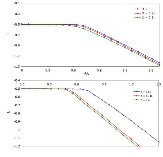
Figure 2: (Color online) Top: Ground state energy for H-atom located at position $\vec{x}=(0,0,Da)$ as a function of $U_{0}$ in units of Hartree. Bottom: Ground state energy of H-atom located at origin as a function of $U_{0}$ in units of Hartree for different thickness values. Here $a$ is $5.75$.

In our simulations we fixed $\Delta\tau\approx 0.05$. ( See the appendix for more details). Throughout the paper, we have implemented the following atomic units. Here and hereafter we use the Bohr radius, $\hbar^{2}/me^{2}=0.529$ Å as the length unit, the value of $\hbar^{3}/me^{4}=2.419\times 10^{-2}$ fs as time unit and the Hartree, $me^{4}/\hbar^{2}=27.25$ eV as the energy unit. The main results of our work are shown in Figures 2-7.

3.1 H-atom endohedrally confined in C₆₀ molecule

First of all we calculated the ground state energy of H-atom endohedrally confined within C₆₀ molecule as a function of $U_{0}$, the confining well strength for different small nuclei positions. The nucleus vector position is considered as $\vec{x}=(0,0,Da)$ where $D$ assumes different values of $0,0.25$ and $0.5$. For off-centered cases, H-atom obviously does not have any spherical symmetry and as expected from an analytical approach, it becomes either more difficult or undoable for such configurations. It is apparently obvious from Fig. 2a that for the small $U_{0}$-values, the ground state energy remains constant at the usual well-known value of -0.5 for ground state energy (-13.6 eV). It means that the electron is not influenced by the outer confining well. For the case of $D=0$, our results are in excellent agreement with recent exact results which were obtained by solving the Schrödinger equation directlyconn2 . From this figure, when the H-atom moves towards to the confining well region, the energy maintains it’s -0.5 value. It then starts to decrease, when it reaches the threshold point at $U_{0}\simeq-0.7$. The value of $U_{0}$ at the threshold point depends on the assumed values of $D$. As physically expected by moving the nucleus of the H-atom far from the shell, the threshold value of $U_{0}$ should move to the right because the atom approaches the free atom case. The effect of thickness for the ground state energy is shown in Fig. 1b with $a=5.75$. The electron of the confined H-atom becomes more immobile when the shell thickness increases. Consequently the electron becomes localized by increasing the shell thickness or the value of the attractive potential. For sake of clarification, the numerical data of the ground state energies are given in the Tables I and II.

The probability of finding the electron at a distance $r$ from its nucleus is proportional to $r^{2}\rho(r)$ where $\rho(r)=\phi(r)\psi_{H}(r)$ and $\phi(r)$ is the electron radial wave function assuming that the nucleus of the H-atom remains at the origin. Fig. 3 depicts the $r\phi(r)$ as a function of $r$ for different $U_{0}$-values. The electron does not feel the effect of the well for small $U_{0}$-values, however it is trapped in the shell region for large $U_{0}$-values. It is important to note that the $r\phi(r)$ does not have any tail for very large attractive potential.

When the H-atom is off-centered, we calculated two-dimensional electron distributions in the $x-z$ plane. Fig. 4 shows the effects of centered $(D=0)$ and off-centered $(D=0.25)$ H-atom on the electron distributions at threshold value of $U_{0}$. In the symmetrical case, electron distribution is uniformly distributed. Our results show that electron distribution has a peak around the nucleus in all directions for a weak attractive potential. However, the electron is localized in the vicinity of the shell region for a strong attractive potential. In this case, the atom becomes ionized depending on the large value of $U_{0}$ and $D$. As it is physically understandable, the electron distributions along $x-$ or $y$-axis holds its symmetry. However the electron distribution along $z$-axis has no symmetry.

3.2 He-atom endohedrally confined in C₆₀ molecule

To the best of our knowledge, there is no analytical solution for He-atom confined within C₆₀ molecules. Recently, some authors have intensively studied the two-electron photoionization cross section of He atom confined in C₆₀.amusia1 They calculated the regular and irregular solutions of the Schrödinger equation for the system. Here we present more accurate ground state energy as well as the associate wave function for the system which will be used to calculate other physical quantities.

We considered a He-atom bounded by fullerene and calculated the ground state properties. The He-atom with its two electrons and nucleus centered at $\vec{x}$ has an anti-symmetric excited state wave function. The method described in this paper allowed us to calculate the ground state energy as functions of attractive potential and the well thickness.

In Fig. 5 we show the ground state energies as a function of attractive energy, $U_{0}$ for different $D$ and thickness values. Similar to the H-atom results, electrons become more immobile with increasing the shell thickness. Note that in the limit of zero $U_{0}$, the ground state energy gets the well-known value of the He ground state energy which is $-2.903$ ($-78.96eV$). The ground state of energy decreases after the threshold $U_{0}\approx-1.9$ value for the centered case and the threshold value is difference from the H-atom problem. Numerical values of ground state energies are given in the Table IV.

Finally, in Fig. 6 we show electron distributions in the $x-z$ plane when nucleus remains at origin for a high value of $U_{0}$. Clearly, two electrons prefer to stay far from each other. Moreover by increasing the value of $U_{0}$, the probability of finding each electron near the shell increases.

4 Concluding remarks

In this work we have numerically calculated the ground state energies and electron distributions of a simple atom confined by C₆₀ fullerene within the diffusion Monte Carlo method. We modeled the C₆₀ fullerene with attractive confining well and obtained the physical quantities of one or two electrons of the atom endohedrally. Our results for a hydrogen atom located at the origin is in excellent agreement with exact calculations. Within the DMC method we obtained the ground state energy for off-centered H- and He-atoms for different confining well potentials. We described the electrons distributions for endohedral case as a function of nucleus positions and the confining well potential as well. Moreover, electron distributions are more influenced by changing the nucleus position. We believe that for an accurate quantitative calculations of off-centered effects, the real physical model for C₆₀ molecule should be deformed in the presence of endohedral atoms and deviation from spherical symmetry should be considered.

Appendix A Details on explicit calculation of the time step

The time step can be selected according to the criterion that the systematic error associated with the use of a finite $\Delta\tau$ is less than the statistical error. To achieve the desired variance in energy, the value of $N_{0}$ and run time are chosen sufficiently large. In these simulations we chose $N_{0}$ and the run time in the range of 4000-6000. In Fig 7. we show the energy and its standard deviation as a function of $\Delta\tau$ for free He-atom. As it is clear from the figure, the range $[0.05-0.1]$ should be the acceptable range of the time step, $\Delta\tau$.

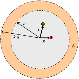
Figure 1: (Color online) The schematic representation of H-atom inside an attractive shell for modeling the H-atom endohedrally confined inside C₆₀ molecules.

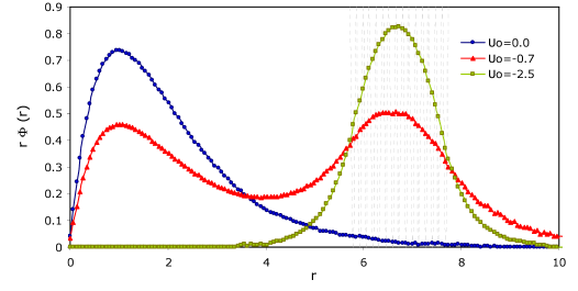
Figure 3: (Color online) Radial electron wave function multiply to position, $r\phi(r)$ as a function of $r$ for H-atom located at $D=0$ for different $U_{0}$ values. Dashed vertical lines refer to the shell region.

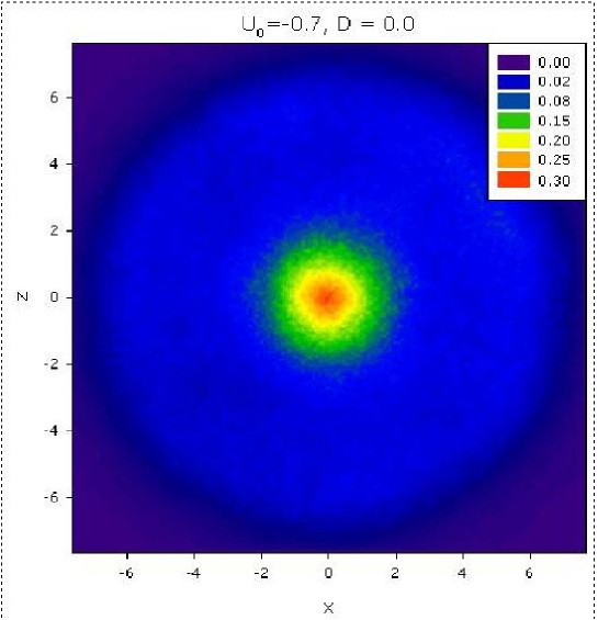
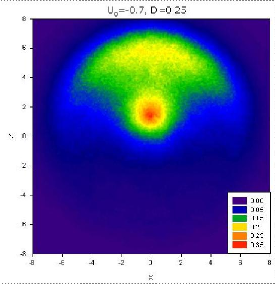
Figure 4: (Color online) Electron distributions of H-atom in $x-z$ plane for $U_{0}=-0.7$ where $D=0.0$ (top) and $D=0.25$ (bottom). Legends denote the number of normalized electron density.

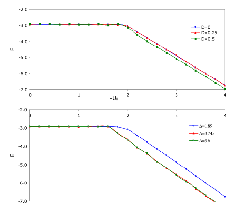
Figure 5: (Color online) Top: Ground state energy of He-atom as a function of $U_{0}$ in units of Hartree. The nuclear is located at $\vec{x}=(0,0,Da)$ for $D=0,0.25$ and $0.5$. Bottom: Ground state energy of He-atom as a function of $U_{0}$ in units of Hartree for different thickness values. Here $a$ is $5.75$.

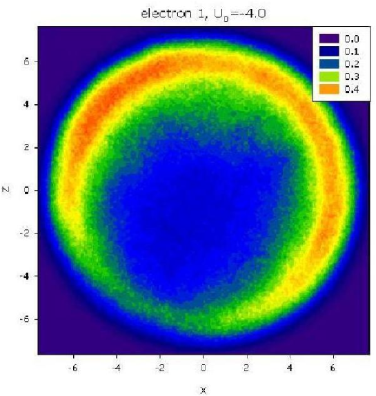
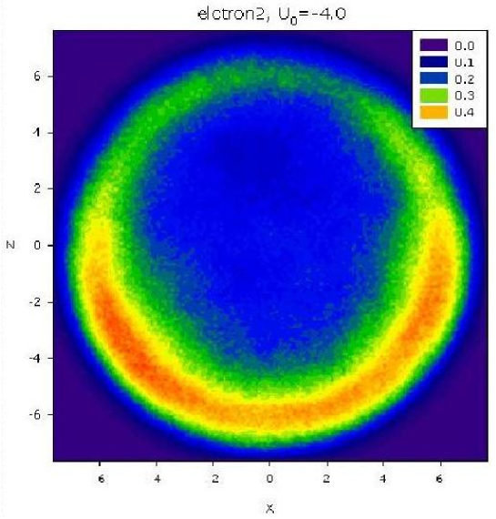
Figure 6: (Color online) Electron distributions in $x-z$ plane for $U_{0}=-4.0$ for two electrons of He-atom confined at $D=0.0$. Legends denote the number of normalized electron density.

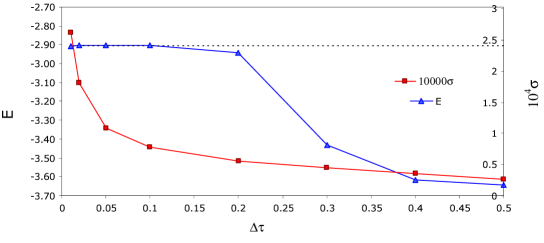
Figure 7: (Color online) Energy (triangle symbol) and standard deviation (square symbol) as a function of time step for free He-atom.

-$U_{0}$	D=0.0	D=0.25	D=0.5
$0.00$	$-0.5000$	$-0.5010$	$-0.5035$
$0.08$	$-0.5011$	$-0.5046$	$-0.5060$
$0.16$	$-0.5017$	$-0.5050$	$-0.5069$
$0.24$	$-0.5019$	$-0.5055$	$-0.5073$
$0.32$	$-0.5023$	$-0.5057$	$-0.5083$
$0.40$	$-0.5027$	$-0.5072$	$-0.5090$
$0.48$	$-0.5032$	$-0.5099$	$-0.5120$
$0.56$	$-0.5039$	$-0.5124$	$-0.5251$
$0.64$	$-0.5053$	$-0.5200$	$-0.5461$
$0.72$	$-0.5255$	$-0.5490$	$-0.5866$
$0.80$	$-0.5789$	$-0.6035$	$-0.6397$
$0.88$	$-0.6388$	$-0.6563$	$-0.6970$
$0.96$	$-0.6998$	$-0.7211$	$-0.7549$
$1.04$	$-0.7628$	$-0.7796$	$-0.8191$
$1.12$	$-0.8271$	$-0.8413$	$-0.8806$
$1.20$	$-0.8934$	$-0.9196$	$-0.9455$
$1.28$	$-0.9585$	$-0.9848$	$-1.0104$
$1.36$	$-1.0259$	$-1.0508$	$-1.0756$
$1.44$	$-1.0938$	$-1.1176$	$-1.1438$
$1.52$	$-1.1619$	$-1.1886$	$-1.2112$
$1.60$	$-1.2311$	$-1.2562$	$-1.2800$

Table 1: Ground state energy for H-atom for different $D$ values. The statistical error bar for GDMC is about $\pm 10^{-4}$.

-$U_{0}$	$\Delta=1.89$	$\Delta=3.745$	$\Delta=5.6$
$0.00$	$-0.5000$	$-0.5000$	$-0.5000$
$0.08$	$-0.5002$	$-0.5003$	$-0.5005$
$0.16$	$-0.5005$	$-0.5007$	$-0.5007$
$0.24$	$-0.5009$	$-0.5011$	$-0.5014$
$0.32$	$-0.5010$	$-0.5014$	$-0.5025$
$0.40$	$-0.5011$	$-0.5015$	$-0.5027$
$0.48$	$-0.5012$	$-0.5062$	$-0.5131$
$0.56$	$-0.5056$	$-0.5409$	$-0.5639$
$0.64$	$-0.5061$	$-0.6100$	$-0.6371$
$0.72$	$-0.5259$	$-0.6824$	$-0.7095$
$0.80$	$-0.5789$	$-0.7544$	$-0.7800$
$0.88$	$-0.6399$	$-0.8238$	$-0.8480$
$0.96$	$-0.7001$	$-0.8965$	$-0.9234$
$1.04$	$-0.7622$	$-0.9718$	$-0.9941$
$1.12$	$-0.8271$	$-1.0437$	$-1.0707$
$1.20$	$-0.8929$	$-1.1128$	$-1.1423$
$1.28$	$-0.9584$	$-1.1907$	$-1.2157$
$1.36$	$-1.0242$	$-1.2637$	$-1.2857$
$1.44$	$-1.0934$	$-1.3390$	$-1.3581$
$1.52$	$-1.1612$	$-1.4142$	$-1.4311$
$1.60$	$-1.2297$	$-1.4819$	$-1.5016$

Table 2: Ground state energy for H-atom for different thickness values.

-$U_{0}$	D=0.0	D=0.25	D=0.5
$0.00$	$-2.9031$	$-2.9036$	$-2.9038$
$0.20$	$-2.9033$	$-2.9045$	$-2.9103$
$0.40$	$-2.9040$	$-2.9057$	$-2.9116$
$0.60$	$-2.9044$	$-2.9063$	$-2.9138$
$0.80$	$-2.9055$	$-2.9077$	$-2.9144$
$1.00$	$-2.9061$	$-2.9088$	$-2.9152$
$1.20$	$-2.9064$	$-2.9145$	$-2.9169$
$1.40$	$-2.9073$	$-2.9188$	$-2.9176$
$1.60$	$-2.9081$	$-2.9231$	$-2.9276$
$1.80$	$-2.9087$	$-2.9424$	$-2.9445$
$2.00$	$-3.0523$	$-3.0560$	$-3.0653$
$2.20$	$-3.4101$	$-3.4148$	$-3.6131$
$2.40$	$-3.7751$	$-3.7756$	$-3.9799$
$2.60$	$-4.1364$	$-4.1441$	$-4.3421$
$2.80$	$-4.5043$	$-4.5053$	$-4.7079$
$3.00$	$-4.8758$	$-4.8705$	$-5.0756$
$3.20$	$-5.2496$	$-5.2502$	$-5.4505$
$3.40$	$-5.6228$	$-5.6228$	$-5.8193$
$3.60$	$-5.9986$	$-5.9976$	$-6.1959$
$3.80$	$-6.3742$	$-6.3767$	$-6.5741$
$4.00$	$-6.7538$	$-6.7494$	$-6.9580$

Table 3: Ground state energy for He-atom for different $D$ values.

-$U_{0}$	$\Delta=1.89$	$\Delta=3.745$	$\Delta=5.6$
$0.00$	$-2.9031$	$-2.9032$	$-2.9032$
$0.20$	$-2.9252$	$-2.9258$	$-2.9263$
$0.40$	$-2.9260$	$-2.9261$	$-2.9265$
$0.60$	$-2.9333$	$-2.9363$	$-2.9372$
$0.80$	$-2.9344$	$-2.9372$	$-2.9394$
$1.00$	$-2.9388$	$-2.9396$	$-2.9429$
$1.20$	$-2.9435$	$-2.9455$	$-2.9468$
$1.40$	$-2.9453$	$-2.9469$	$-2.9479$
$1.60$	$-2.9559$	$-2.9614$	$-2.9738$
$1.80$	$-2.9657$	$-3.2565$	$-3.2902$
$2.00$	$-3.0823$	$-3.6351$	$-3.6563$
$2.20$	$-3.4101$	$-4.0522$	$-4.0453$
$2.40$	$-3.7751$	$-4.4060$	$-4.3871$
$2.60$	$-4.1364$	$-4.8250$	$-4.8418$
$2.80$	$-4.5043$	$-5.1915$	$-5.1753$
$3.00$	$-4.8758$	$-5.5377$	$-5.5693$
$3.20$	$-5.2496$	$-5.8922$	$-5.9155$
$3.40$	$-5.6228$	$-6.3206$	$-6.2839$
$3.60$	$-5.9986$	$-6.6892$	$-6.6714$
$3.80$	$-6.3742$	$-7.0863$	$-7.0453$
$4.00$	$-6.7538$	$-7.4316$	$-7.4289$

Table 4: Ground state energy for He-atom for different thickness values.

References

- (1) H. W. Kroto, J. R. Heath, S. C. O’Brien, R. F. Smalley, Nature (London) 318 (1985) 162 .
- (2) M. Häser, J. Almlöf and G. E. Scuseria, Chem. Phys. Lett. 181 (1991) 497 .
- (3) B. I. Dunlap, D. W. Brenner, J. W. Mintmire, R. C. Mowrey and T. C. White, J. Phys. Chem. 95 (1991) 8737 .
- (4) H. Heggie, M. Terrones, B. R. Egger, G. Jungnickel, R. Jones, C. D. Latham, P. R. Briddon and H. Terrones, Phys. Rev. B 57 (1998) 13339 .
- (5) H. Shinohara, Rep. Prog. Phys. 63 (2000) 843; L. Forro’ and L. Miha’ly, Rep. Prog. Phys. 64 (2001) 649 .
- (6) V. K. Dolmatov and S. T. Manson, Phys. Rev. A 73 (2006) 013201 .
- (7) M. Ya. Amusia, E. Z. Liverts and V. B. Mandelzweing, Phys. Rev. A 74 (2006) 042712 .
- (8) J. P. Connerade and A. V. Solov’yov, J. Phys. B 38 (2005) 807; J. P. Connerade, V. K. Dolmatov and S. T. Manson, J. Phys. B 33 (2000) 2279 .
- (9) Jerzy Cioslowski and Eugene D. Fleischmann, J. Chem. Phys. 94 (1991) 3730 .
- (10) A. C. Dillon, K. M. Jones, T. A. Bekkedahl, C. H. Kiang, D. S. Bethune and M. J. Heben, Nature (London) 386 (1997) 377 .
- (11) W. Liang, M. Bockrath and H. Park, Phys. Rev. Lett. 88 (2002) 126801 .
- (12) Y. Zhao, Y-H. Kim, A. C. Dillon, M. J. Heben, and S. B. Zhang, Phys. Rev. Lett. 94 (2005) 155504 .
- (13) M. J. Puska , and R. M. Nieminen, Phys. Rev. A 47 (1993) 1181 .
- (14) Y. B. Xu, M. Q. Tan, and U. Becker, Phys. Rev. Lett. 76 (1996) 3538 .
- (15) J. P. Connerade , V. K. Dolmatov, P. A. Lakshmi and S. T. Mansonk, J. Phys. B 32 (1999) L239 .
- (16) K. D. Sen, J. Chem. Phys. 122 (2005) 194324 .
- (17) J. P Connerade and R. Semaoune, J. Phys. B 33 (2000) 869 .
- (18) M. Ya. Amusia, A. S. Baltenkov, and U. Becker, Phys. Rev. A. 62 (2000) 012701 .
- (19) J. B. Anderson, J. Chem. Phys. 63 (1975) 1499 .
- (20) P. J. Reynolds, D. M. Ceperely, B. J. Alder and W. A. Lester Jr., J. Chem. Phys. 77 (1982) 5593; J. Vrbik and S. M. Rohtstein, J. Comput. Phys. 63 (1986)130; I. Kosztin, B. Faber and K. Schulten, Am. J. Phys. 64 (1996) 633 .
- (21) P. R . Charles Kent, 1999, Ph.D. thesis, University of Cambridge.
- (22) W. M. C. Foulkes, L. Mitas, R. J. Needs and G. Rajagopal, Rev. Mod. Phys. 73 (2001) 33 .
- (23) C. Joslin and S. Goldman, J.Phys. B: At. Mol. Opt. Phys. 25 (1592) 1965-1975.