Inelastic scattering from quantum impurities

Abstract

We review the non-perturbative theoretical framework set up recently to compute the inelastic scattering cross section from quantum impurities [G. Zaránd et al., Phys. Rev. Lett. 93, 107204 (2004)] and show how it can be applied to a number of quantum impurity models. We first use this method for the $S=1/2$ single-channel Kondo model and the Anderson model. In both cases, a large plateau is found in the inelastic scattering rate for incoming energies above $T_{K}$, and a quasi-linear regime appears in the energy range $0.05\;T_{K}<\omega<0.5\;T_{K}$, in agreement with the experimental observations. We also present results for the 2-channel Kondo model, the prototype of all non-Fermi liquid models, and show that there half of the scattering remains inelastic even at the Fermi energy.

1 Introduction

One of the major ingredients of mesoscopic physics is quantum interference: it leads to phenomena such as weak localization, Aharonov-Bohm interference, universal conductance fluctuations, or mesoscopic local density of states fluctuations [1]. All these phenomena rely on the phase coherence of the conduction electrons. This phase coherence is, however, destroyed through inelastic scattering processes, where an excitation is created in the environment. These inelastic processes suppress quantum interference after the so-called dephasing time, $\tau_{\varphi}$, also called inelastic scattering time. The excitations created in course of an inelastic scattering process may be phonons, magnons, electromagnetic radiation, or simply electron-hole excitations.

A few years ago Mohanty and Webb measured the dephasing time $\tau_{\varphi}(T)$ carefully down to very low temperatures through weak localization experiments, and reported a surprising saturation of it at the lowest temperatures [2]. These experiments gave rise to many theoretical speculations: intrinsic dephasing due to electron-electron interaction [3] as well as scattering from two-level systems [4, 5] have been proposed to explain the observed saturation, and induced rather violent discussions [3, 6, 7]. Recently, it has been finally proposed that an apparent saturation could well be explained by inelastic scattering from magnetic impurities [8, 9].

Triggered by these results of Mohanty and Webb, a number of experimental groups also revisited the problem of inelastic scattering and dephasing in quantum wires and disordered metals: A series of experiments have been performed to study the non-equilibrium relaxation of the energy distribution function in short quantum wires [10]. These energy relaxation experiments could be well explained in terms of the orthodox theory of electron-electron interaction in one-dimensional wires [11], and/or inelastic scattering mediated by magnetic impurities [12, 13, 14, 15]. Parallel to, and partially triggered by these experiments, a systematic study of the inelastic scattering from magnetic impurities has also been carried out recently, where inelastic scattering from magnetic impurities at energies down to well below the Kondo scale has also been studied [16, 17, 18].

Theoretically, this strong coupling regime can be reached only through a non-perturbative approach. Such a method to compute the inelastic scattering cross-section has been proposed in Ref. [9] and further developed in Ref [19], where it has been shown that the finite temperature version of the formula introduced in Ref. [9] describes indeed the dephasing rate that appears in the expression of weak localization in the limit of small concentrations. Except for very low temperatures, where a small residual inelastic scattering is observed [17, 18], these calculations were in excellent agreement with the experiments, and they clearly showed that magnetic impurities in concentration as small as 1ppm can already induce substantial inelastic scattering. We have to emphasize though that experiments on very dirty metals, e.g., probably cannot be explained in terms of magnetic scattering, and possibly other mechanisms are needed to account for the dephasing observed at very low temperatures in these systems [20].

Here we review the theory of Ref. [9] and show how it can be applied to various quantum impurity problems. In Ref. [9] we formulated the problem of inelastic scattering in terms of the many-body $S$-matrix defined through the overlap of incoming and outgoing scattering states:

$$\phantom{a}{}_{\textrm{out}}\langle f|i\rangle_{\textrm{in}}\equiv\phantom{a}_{\textrm{in}}\langle f|\hat{S}|i\rangle_{\textrm{in}}\;.$$ (1)

The incoming and outgoing scattering states, $|i\rangle_{\textrm{in}}$ and $|f\rangle_{\textrm{out}}$, are asymptotically free, however, they may contain many excitations, i.e. they are true many-body states. The many-body $T$-matrix is defined as the ’scattering part’ of the $S$-matrix, $\hat{S}=\hat{I}+i\hat{T}$, with $\hat{I}$ the identity operator. By energy conservation

$${}_{\textrm{in}}\langle f|\hat{T}|i\rangle_{\textrm{in}}=2\pi\;\delta(E_{f}-E_{i})\;\langle f|{\cal T}|i\rangle\;,$$ (2)

where we introduced the on-shell $T$-matrix $\langle f|{\cal T}|i\rangle$. The results of Ref. [9] rely on the simple observation, that $\langle{\bf p}\sigma|{\cal T}|{\bf p^{\prime}}\sigma^{\prime}\rangle$ determine both the total ($\sigma_{\rm tot}$) and the elastic ($\sigma_{\rm el}$) scattering cross sections of the conduction electrons (or holes) at $T=0$ temperature. The total scattering cross section of an electron of momentum ${\bf p}$ and spin $\sigma$ is given by the optical theorem as

$$\sigma_{\rm total}^{\sigma}=\frac{2}{v_{F}}{\rm Im}\langle{\bf p}\sigma|{\cal T}|{\bf p}\sigma\rangle\;,$$ (3)

where $v_{F}$ denotes the Fermi velocity. This expression accounts also for processes where a single electron scatters into many excited electron states (see Fig. 1). In case of elastic scattering, on the other hand, an incoming single electron state is scattered into an outgoing single electron state, without inducing any spin or electron-hole excitation of the environment. The corresponding cross section can be expressed as

$$\sigma_{\rm el}^{\sigma}=\frac{1}{v_{F}}\int{\frac{d{\bf p}^{\prime}}{(2\pi)^{3}}}2\pi\;\delta(\xi^{\prime}-\xi)|\langle{\bf p}^{\prime}\sigma|{\cal T}|{\bf p}\sigma\rangle|^{2}\;,$$ (4)

with $\xi$ the energy of the electron measured from the Fermi surface. Inelastic scattering processes, schematically illustrated in Fig. 1, can be defined as scattering processes, which are not elastic. Accordingly, the inelastic scattering cross section associated with these processes is just the difference of these two cross-sections:

$$\sigma_{\rm inel}^{\sigma}=\sigma_{\rm total}^{\sigma}-\sigma_{\rm el}^{\sigma}\;.$$ (5)

This simple formula allows us to compute the inelastic scattering cross-section in detail.

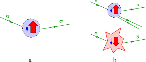
Figure 1: Sketch of (a) elastic and (b) inelastic scattering processes. In case of an inelastic scattering the outgoing electron leaves spin- and/or electron-hole excitations behind.

In a free electron gas it is convenient to introduce angular momentum channels, $L\equiv(l,m)$, and define the scattering states in terms of radially propagating states $|{\bf p},\sigma\rangle\to||{\bf p}|,L,\sigma\rangle$. In this basis the on-shell $S$ and $T$-matrices become matrices in the quantum numbers $L$, and they depend only on the energy $\omega$ of the incoming particle [21],

$${s}_{L,\sigma;\;L^{\prime}\sigma^{\prime}}(\omega)=\delta_{L,L^{\prime}}\delta_{\sigma,\sigma^{\prime}}+i\;{t}_{L,\sigma;\;L^{\prime}\sigma^{\prime}}(\omega)\;.$$ (6)

By unitarity, the eigenvalues $s_{\lambda}$ of the matrix $s_{L,\sigma;\;L^{\prime}\sigma^{\prime}}$ must all be within the complex unit circle for any $\omega$, and they are directly related to the inelastic scattering cross section. In case of $s$-scattering and spin-conservation, e.g., $s_{L,\sigma;\;L^{\prime}\sigma^{\prime}}$ becomes a simple number, $s(\omega)=1+i\;t(\omega)$, and the inelastic scattering cross section can be expressed as

$$\sigma_{\rm inel}(\omega)=\frac{\pi}{p_{F}^{2}}\;(1-|{s}(\omega)|^{2})=\frac{\pi}{p_{F}^{2}}\;(2\;{\rm Im}\;t(\omega)-|t(\omega)|^{2})\;,$$ (7)

where we assumed free electrons of dispersion $\xi={\bf p}^{2}/2m-\mu$ with a Fermi energy $\mu$ and a corresponding Fermi momentum $p_{F}$. Eq. (7) implies that the scattering becomes totally elastic whenever ${s}(\omega)$ is on the unit circle, and it is maximally inelastic if the corresponding single particle matrix element of the $S$-matrix vanishes. The former situation occurs at Fermi liquid fixed points, while the latter case is realized, e.g., in case of the two-channel or the two-impurity Kondo models. The total scattering cross section, on the other hand, is related to the real part of ${s}(\omega)$ as

$$\sigma_{\rm tot}(\omega)=\frac{2\pi}{p_{F}^{2}}\;(1-{\rm Re}\{{s}(\omega)\})=\frac{2\pi}{p_{F}^{2}}\;{\rm Im}\{{t}(\omega)\}\;.$$ (8)

It is easy to generalize this result to the case of many scattering channels, and one finds that inelastic scattering can take place only if some of the eigenvalues of $s_{L,\sigma;\;L^{\prime}\sigma^{\prime}}$ are not on the unit circle [31].

To determine $t_{L\sigma,L^{\prime}\sigma^{\prime}}$ we need to compute the matrix element $\langle{\bf p}\sigma|{\cal T}|{\bf p}^{\prime}\sigma^{\prime}\rangle$, that we first relate to the conduction electrons’ Green function through the so-called reduction formula [21, 22],

$$\langle{\bf p},\sigma|{\cal T}|{\bf p}^{\prime}\sigma^{\prime}\rangle=-\;[G^{0}]^{-1}_{\pm{\bf p},\pm\sigma}(\xi)\;G_{\pm{\bf p}\;\pm\sigma,\pm{\bf p}^{\prime}\;\pm\sigma^{\prime}}(\xi)\;[G^{0}]^{-1}_{\pm{\bf p}^{\prime}\pm\sigma^{\prime}}(\xi)\;.$$ (9)

Here the $\pm$ signs correspond to electron and hole states with $\xi>0$ and $\xi<0$ and of energy $E=|\xi|$, $G_{0}$ denotes the free electron Green’s function, and $G$ the full many-body time-ordered electron Green’s function. By Eq. (9) the positive frequency part of the Green’s function describes the scattering of electrons, while the negative frequency part that of holes. In case of a degenerate vacuum state one must average over the various vacuum states in Eq. (9) [31, 19].

According to Eqs. (3), (4), (5), and (9), to compute the inelastic and elastic scattering cross-sections, we only need to evaluate the self-energy of the conduction electron’s Green function, many cases referred to as the $T$-matrix. This can be done either analytically using, e.g., perturbative methods, or numerically, by relating the self-energy to some local correlation function, and computing the latter by Wilson’s numerical renormalization group (NRG) method [34]. The latter approach enables us to compute both the imaginary and real parts of the matrix $t(\omega)$, and we can thus also determine the complex eigenvalue $s(\omega)$.

2 Inelastic scattering in the Kondo model

Let us first apply this formalism to study the inelastic scattering in the single-channel Kondo model defined by the Hamiltonian

$$H=\sum_{{\bf p},\sigma}\xi_{\bf p}\;a^{\dagger}_{{\bf p}\sigma}a_{{\bf p}\sigma}+\frac{J}{2}\vec{S}\sum_{{\bf p},{\bf p}^{\prime}\atop\sigma\sigma^{\prime}}a^{\dagger}_{{\bf p}\sigma}{\vec{\sigma}}_{\sigma\sigma^{\prime}}a_{{\bf p}^{\prime},\sigma^{\prime}}\;.$$ (10)

Here $a^{\dagger}_{{\bf p}\sigma}$ creates a conduction electron with momentum $\bf p$, spin $\sigma$, and $S=1/2$ is the impurity spin. The $T$-matrix of the Kondo model can be related to the Green’s function of the so-called composite Fermion operator, $F_{\sigma}\equiv\sum_{\sigma^{\prime},{\bf p}}{\vec{S}}\cdot{\vec{\sigma}}_{\sigma\sigma^{\prime}}a_{{\bf p}\sigma^{\prime}}$ [30], whose spectral function can then be computed using NRG [34].

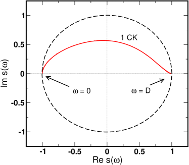
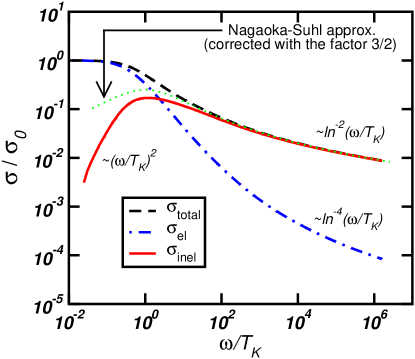
Figure 2: Left: Renormalization group flow of the eigenvalue of the single particle $S$-matrix for the single-channel Kondo model. Right: Energy-dependence of the elastic-, total- and inelastic scattering rates for the Kondo model.

Before presenting our numerical results, let us briefly discuss what we can learn about the inelastic scattering cross-section from analytical approaches. The $\omega\gg T_{K}$ regime is accessible by perturbation theory. Summing up the leading logarithmic diagrams we find

$$t(\omega\gg T_{K})\approx i\;({\pi^{2}}/2)S(S+1)/{\ln^{2}(\omega/T_{K})}\;,$$ (11)

where $T_{K}\sim E_{F}e^{-1/J\varrho}$ is the Kondo temperature, with $E_{F}$ the Fermi energy and $\varrho$ the density of states at the Fermi energy for one spin direction [29]. To leading logarithmic order, the scattering is completely inelastic

$$\sigma_{\rm inel}(\omega\gg T_{K})\approx\sigma_{\rm tot}(\omega)\approx\frac{\pi^{3}}{p_{F}^{2}}\;S(S+1)\frac{1}{\ln^{2}(\omega/T_{K})}\;,$$ (12)

since the elastic contribution only increases as $\sigma_{\rm el}\sim|t(\omega)|^{2}$,

$$\sigma_{\rm el}(\omega\gg T_{K})\approx\frac{\pi^{5}}{4\;p_{F}^{2}}\;S^{2}(S+1)^{2}\frac{1}{\ln^{4}(\omega/T_{K})}\;.$$ (13)

This very surprising result contradicts conventional wisdom, which tries to associate inelastic scattering with spin-flip scattering. It can be explained in the following way [24]: At high energies, incoming electrons are scattered by the impurity spin fluctuations. These fluctuations can absorb an energy of the order of $\sim T_{K}$, and therefore the energy of the incoming electron is not conserved even in leading order, but it typically changes by a tiny amount, $\delta\omega\sim T_{K}$. In earlier approaches, this tiny energy transfer has been neglected, and the spin-diagonal scattering has been incorrectly identified as an elastic process.

We can also relate the cross sections above to scattering rates. Assuming a finite but small concentration $n_{\rm imp}$ of magnetic impurities, the conduction electrons’ lifetime can be expressed as $1/\tau(\omega)=n_{\rm imp}\;v_{F}\;\sigma_{\rm imp}(\omega)$. This relation can be used to define the inelastic scattering rate too as

$$\frac{1}{\tau_{\rm inel}}\equiv n_{\rm imp}\;v_{F}\;\sigma_{\rm inel}(\omega)\approx n_{\rm imp}\frac{\pi S(S+1)}{2\;\varrho\;\ln^{2}(\omega/T_{K})}\;,\phantom{nn}(\omega\gg T_{K}).$$ (14)

Note that the latter asymptotic expression is a factor 3/2 larger than the Nagaoka-Suhl formula, which takes into account only spin-flip processes [33].

For energies $|\omega|<T_{K}$ perturbation theory breaks down, and it is more appropriate to use Nozières’ Fermi liquid theory, according to which scattering at Fermi energy scattering is completely elastic, and is described through simple phase shifts [23], $t_{\sigma}(\omega=0^{+})=2\sin\delta_{\sigma}\;e^{i\delta_{\sigma}}$. Here we allowed for different phase shifts in the spin up and spin down channels. This Fermi liquid expression yields

$$\sigma_{\rm tot,\sigma}(\omega\to 0)=\frac{4\pi}{p_{F}^{2}}\sin^{2}(\delta_{\sigma})\;,\phantom{nnnnnnnn}\sigma_{\rm inel,\sigma}(\omega\to 0)=0\;.$$ (15)

The maximum total scattering cross section is reached in the unitary limit, $\delta_{\sigma}=\pi/2$, while the inelastic scattering cross-section always vanishes at the Fermi energy. Perturbation theory around the Fermi liquid fixed point predicts $\sigma_{\rm inel,\sigma}(\omega\to 0)\propto(\omega/T_{K})^{2}$ [9, 25].

The analytical calculations above can only capture the physics in the limit of very large and very small frequencies, and for energies $\omega\sim T_{K}$ we need to use more sophisticated methods such as NRG. In Fig. 2 we show the evolution of the eigenvalue of the $s(\omega)$. In the limit $T_{K}/E_{F}\ll 1$ this becomes a universal function, ${s}(\omega)={s}(\omega/T_{K})$. In the single-channel Kondo model $|{s}(\omega)|\to 1$ for both very large and very small frequencies, and thus scattering becomes completely elastic both limits. The reasons are different: At large energies conduction electrons do not interact with the impurity spin efficiently. At very small energies, on the other hand, the impurity’s spin is screened and disappears from the problem [23]. The maximum inelastic scattering is reached when the eigenvalue ${s}(\omega)$ is closest to the origin, i.e., at energies in the range of the Kondo temperature, $\omega\approx T_{K}$.

The total, elastic and inelastic scattering cross sections of an electron are shown in Fig.3. As expected, the inelastic amplitude always vanishes at the Fermi level, and at energies well above $T_{K}$ both the elastic and the inelastic scattering cross-sections follow the the analytical expressions, Eqs. (12) and (13). For energies $|\omega|\ll T_{K}$ we recover the quadratically vanishing inelastic rate expected from Fermi liquid theory [25], but the $\sigma_{\rm inel}\sim\omega^{2}$ regime appears only at energies well below the Kondo temperature, $\omega<0.05\;T_{K}$ (see Fig.3). For $|\omega|\gg T_{K}$ the usual Nagaoka-Suhl expression describes the inelastic scattering rather well apart from the incorrect overall pre-factor 3/2 discussed before, but it starts to deviate strongly from the numerically exact curve at approximately $10\;T_{K}$, and it completely fails below the Kondo temperature $T_{K}$.

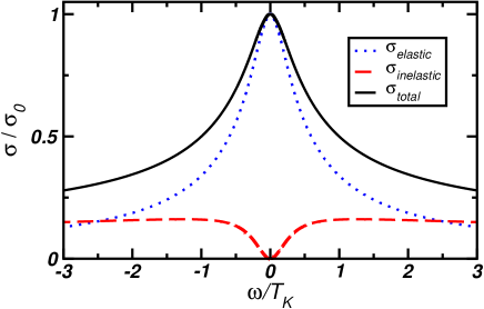
Figure 3: Inelastic, elastic, and total scattering rates for the single-channel Kondo model in units of $\sigma_{0}=4\pi/p_{F}^{2}$, as a function of the incoming electron’s energy.

Interesting features appear also at intermediate temperatures. The inelastic scattering rate is roughly linear between $0.05\;T_{K}<\omega<0.5\;T_{K}$, and a broad plateau appears above the Kondo scale, where the energy-dependence of the inelastic scattering rate turns out to be extremely weak. Even though our calculation is done at $T=0$ temperature, $\sigma_{\rm inel}(T,\omega=0)$ is expected to behave very similarly to $\sigma_{\rm inel}(T=0,\omega)$. Thus both features are perfectly consistent with several experiments [26, 16, 8], and, somewhat surprisingly, our results fit the experimentally measured temperature-dependence of $1/\tau_{\Phi}$ excellently [16]. This is beyond expectations, since realistic magnetic impurities have a complicated $d$-level structure, and our $T=0$ temperature results provide just approximations for the dephasing rate, and one should use the finite temperature expression of the dephasing rate, computed in Ref. [19].

3 Anderson model

Let us next discuss the Anderson model, defined by the Hamiltonian,

$$H=\sum_{{\bf p}\sigma}\epsilon({\bf p})a^{\dagger}_{{\bf p}\sigma}a^{\phantom{\dagger}}_{{\bf p}\sigma}+\epsilon_{d}\sum_{\sigma}d^{\dagger}_{\sigma}d^{\phantom{\dagger}}_{\sigma}+Ud^{\dagger}_{\uparrow}d^{\phantom{\dagger}}_{\uparrow}d^{\dagger}_{\downarrow}d^{\phantom{\dagger}}_{\downarrow}+V\sum_{\sigma,{\bf p}}\left(c^{\dagger}_{{\bf p}\sigma}d^{\phantom{\dagger}}_{\sigma}+\textrm{h.c.}\right)\;.$$

Here $d_{\sigma}$ denotes a local $d$-level’s annihilation operator, $U$ is the on-site Coulomb repulsion, and the conduction band and the local electronic level are hybridized by $V$. The Anderson model is the most elementary Hamiltonian that describes local moment formation on a localized $d$-orbital, and in fact, the Kondo Hamiltonian can be obtained from it in the limit $\Delta\ll U+\epsilon_{d},|\epsilon_{d}|$, with $\Delta=\pi\varrho V^{2}$ the width of the resonance [29].

As first discussed by Langreth [27], the $T$-matrix for the Anderson model can be related to the $d$-level’s Green’s function as [9, 29]

$${\rm Im}\{{\cal T}_{\sigma}(\omega)\}=\pi{V^{2}}\varrho_{d,\tau\sigma}(\omega)\;,\phantom{nn}{\rm Re}\{{\cal T}_{\sigma}(\omega)\}=-\tau\;{V^{2}}\int d\omega^{\prime}\;\frac{\varrho_{d,\tau\sigma}(\omega)}{\omega-\omega^{\prime}}\;.$$

Here $\tau={\rm sgn}\;\omega$, and $\varrho_{d,\sigma}(\omega)$ is the spectral function of the $d$-Fermion, which we have computed using NRG [21].

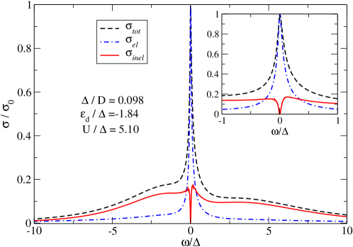
Figure 4: Elastic, inelastic and total scattering cross section for the asymmetric Anderson model. The low-energy part of the curves is very similar to the one obtained for the Kondo model.

The full frequency-dependence of the various scattering cross-sections obtained for the asymmetrical Anderson model with interaction strength $U/\Delta=5.1$ is shown in Fig. 4. At this value of $U$ one can already observe the Hubbard side-peaks in the total scattering cross section at energies $\omega\approx\epsilon_{d}$ and $\omega\approx U+\epsilon_{d}$, and a distinct Kondo resonance appears at $\omega\approx 0$ too. The scattering rates in the region $\omega\approx 0$ are strikingly similar to the ones we obtained for the Kondo model, and remarkably, both the quasi-linear regime of $\sigma_{\rm inel}$ and the plateau are already present for these moderate values of $U/\Delta$. This is not very surprising since, as stated before, the Kondo model is just the effective model of the Anderson model in the limit of large $U/\Delta$ and $\omega\ll U$. For even larger values of $U/\Delta$ and intermediate energies, $T_{K}\ll\omega\ll U$, the elastic and inelastic contributions follow very nicely the asymptotic behavior found for the Kondo model, and scale as $\sim 1/\ln^{4}(\omega/T_{K})$ and $\sim 1/\ln^{2}(\omega/T_{K})$, respectively. New features compared to the Kondo model are the Hubbard peaks that correspond almost entirely to inelastic scattering.

4 Inelastic scattering in the two-channel Kondo model

So far, we considered scattering from Fermi liquid models only. Let us now discuss the two-channel Kondo model, the prototype of all non-Fermi liquid impurity models [28]. This is defined by a Hamiltonian similar to Eq. (10) excepting that now there is two ’channels’ of conduction electrons, $\alpha=1,2$ that are coupled to the impurity spin with couplings $J_{\alpha}$,

$$H=\sum_{\alpha=1,2}\sum_{{\bf p},\sigma}\xi_{\bf p}\;a^{\dagger}_{{\bf p}\sigma,\alpha}a_{{\bf p}\sigma,\alpha}+\sum_{\alpha=1,2}\frac{J_{\alpha}}{2}\vec{S}\sum_{{\bf p},{\bf p}^{\prime}\atop\sigma\sigma^{\prime}}a^{\dagger}_{{\bf p},\alpha}{\vec{\sigma}}_{\sigma\sigma^{\prime}}a_{{\bf p}^{\prime},\alpha}\;.$$ (16)

In the channel-symmetric case, $J_{1}=J_{2}$ the two conduction electron channels compete to screen the impurity spin independently, which is therefore never completely screened. This competition leads to the formation of a strongly correlated state which cannot be described by Nozières’ Fermi liquid theory, and is characterized by a non-zero residual entropy, the logarithmic divergence of the impurity susceptibility, and the power law behavior of transport properties with fractional exponents [28]. Any infinitesimal asymmetry in the couplings $\Delta=(J_{1}-J_{2})/(J_{1}+J_{2})$ leads to the appearance of another low-temperature energy scale $T^{*}\propto\Delta^{2}\;T_{K}/$ at which the system crosses over to a Fermi liquid behavior: Electrons being more strongly coupled to the impurity form a usual Kondo singlet with the impurity spin, while the other electron channel becomes completely decoupled from the spin.

For $J_{1}=J_{2}$, no Fermi-liquid relations are available. There exists, however, an exact theorem due to Maldacena and Ludwig, according to which, at the two-channel Kondo fixed point, the single-particle elements of the $S$-matrix identically vanish for $\omega\to 0$: $s_{2CK}(\omega\to 0)=0$ [32]. As a consequence, $t_{2CK}(\omega=0)=-i\;.$ This relation leads to the surprising result that exactly half of the scattering is inelastic at the Fermi energy, while the other half of it is inelastic:

$$\sigma_{\rm inel}^{\rm 2CK}(\omega=0)=\sigma_{\rm el}^{\rm 2CK}(\omega=0)={\sigma_{\rm tot}^{\rm 2CK}(\omega=0)}/2\;.$$ (17)

This counter-intuitive result can be understood as follows: The vanishing of the single particle $S$-matrix indicates that an incoming electron cannot be detected as one electron after the scattering event, and it “decays” into infinitely many electron-hole pairs. To get such a “decay”, however, the scattering process must have an elastic part which interferes destructively with the unscattered direct wave, and cancels exactly the outgoing single particle amplitude in the $s$-channel.

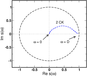
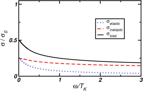
Figure 5: Left: Renormalization group flow of the eigenvalue of the single particle $S$-matrix for the two-channel Kondo model. Right: Energy-dependence of elastic and inelastic scattering rates for the two-channel Kondo model in units of $\sigma_{0}=4\pi/p_{F}^{2}$, at $T=0$.

The evolution of $s(\omega)$ and the inelastic scattering rates for the two-channel Kondo model are shown in Fig. 5 as a function of the energy of the incoming particle. In the channel-symmetric case inelastic processes are allowed even at $\omega=0$, which is a clear signature of the non-Fermi liquid behavior. The non-Fermi liquid nature is also reflected in the $\sim\sqrt{\omega}$ singularity of the scattering cross sections at $\omega=0$.

For $\Delta>0$ the total scattering rate approaches the unitary limit in channel “1” below the Fermi liquid scale $T^{*}$, while it goes to 0 for $\Delta<0$. In both cases, the inelastic scattering freezes out, $\sigma_{\rm inel}(\omega)$ shows a dip below $T^{*}$, and it ultimately scales to 0 as

$$\sigma_{\rm inel}(\omega)\propto{\omega^{2}}/{{T^{*}}^{2}}\;.$$

Remarkably, the inelastic scattering cross-section is very similar for $\Delta>0$ and $\Delta<0$, while the scattering contributions are dramatically different in these two cases (see Ref. [21]).

5 Conclusions

In the present paper we reviewed a recent theory of inelastic scattering from quantum impurities, and applied it to the single and two-channel Kondo models, and the Anderson model.

We showed that in the Kondo model and in the local moment regime of the Anderson model a broad plateau appears in the $T=0$ temperature energy-dependent inelastic scattering rate above $T_{K}$, while a quasi-linear regime emerges below $T_{K}$, in the $T=0$ temperature, both in excellent agreement with recent experimental observations. We also computed the universal flow of the eigenvalues of the $S$-matrix, which is a useful quantity to classify various types of impurity states [31].

As an example of a non-Fermi liquid, we also discussed scattering from the two-channel Kondo model, where half of the scattering remains inelastic even at the Fermi energy, and correspondingly, the eigenvalue of the $S$-matrix vanishes. This fragile non-Fermi liquid state is, however, destroyed, once a small channel-symmetry breaking is applied, and then the scattering becomes elastic below a Fermi-liquid scale, $T^{\star}$ [21].

Our results have been extended to $T\neq 0$ temperatures by Micklitz et al. in Ref. [19], who showed that the dephasing time can indeed be related to the inelastic cross-section computed here for $T=0$ temperature. The theory presented here has also been applied by Koller et al. to the $S=1$ Kondo model [35]. This under-screened model represents a singular Fermi liquid [31], where the scattering is elastic at the Fermi energy, however, it scales to 0 only logarithmically, in contrast to a Fermi liquid.

Let us close our conclusions with an important remark. In a real experiment, the external electromagnetic field couples with a minimal coupling to the conduction electrons. As a consequence, the Kubo formula is formulated in terms of the conduction electron current operators, and the relevant quantity to determine dephasing is thus the inelastic scattering rate of electrons. This is what we compute here and that has been computed in Ref. [19]. Quasiparticles are, on the other hand, typically not minimally coupled to the guage field, since they are usually complicated objects in terms of conduction electrons. If one defines quasiparticles as stable elementary excitations of the vacuum, as Nozières did [23], or as they appear in Bethe Ansatz, then, by definition, these quasiparticles do not decay at all at $T=0$ and scatter only elastically [23]. However, excepting for $\omega=0$, a real conduction electron is composed of many such stable quasiparticles, and it already decays inelastically even at $T=0$ temperature. In the Kondo model, at the Fermi energy quasiparticle states are just phase shifted conduction electron states, however, the connection between quasiparticles and conduction electrons is not trivial for any finite energy. Therefore, if one considers inelastic scattering at a finite energy, one must precisely specify how finite energy quasiparticle states are defined, how they couple to a guage field, and how a finite energy electronic state is decomposed in terms of these quasiparticles,. In the present framework, we avoid this difficulty by formulating the problem in terms of electrons.

We are indebted to L. Saminadayar, C. Bäuerle, J.J. Lin, and A. Rosch for valuable discussions. This research has been supported by Hungarian grants Nos. NF061726, D048665, T046303 and T048782. L.B. acknowledges the financial support of the Bolyai Foundation.

References

- [1] For a review see,e.g., B.L. Altshuler, in Les Houches Lecture Notes on Mesoscopic Quantum Physics (edited by A. Akkermans et al., Elsevier, 1995).
- [2] P. Mohanty, E. M. Q. Jariwala, and R. A. Webb, Phys. Rev. Lett. 78, 3366 (1997).
- [3] D. S. Golubev and A. D. Zaikin, Phys. Rev. Lett. 81, 1074 (1998); See also the criticism in
- [4] A. Zawadowski, J. von Delft, and D. C. Ralph, Phys. Rev. Lett. 83, 2632 (1999).
- [5] Y. Imry, H. Fukuyama and P. Schwab, Europhys. Lett. 47, 608 (1999).
- [6] I. L. Aleiner, B. L. Altshuler and M. E. Gershenson, Waves in Random Media 9, 201 (1999).
- [7] J. von Delft, cond-mat/0510563; J. von Delft, in Fundamental Problems of Mesoscopic Physics, edited by I.V. Lerner et al. (Kluver, London, 2004), p.115-138.
- [8] F. Pierre, A. B. Gougam, A. Anthore, H. Pothier, D. Esteve, and N. O. Birge, Phys. Rev. B 68, 085413 (2003).
- [9] G. Zaránd, L. Borda, J. von Delft and N. Andrei, Phys. Rev. Lett. 93, 107204 (2004).
- [10] H. Pothier, S. Guéron, N. O. Birge, D. Esteve, and M. H. Devoret, Phys. Rev. Lett. 79, 3490 (1997).
- [11] B. L. Altshuler, A. G. Aronov, and D. E. Khmelnitskii, J. Phys. C 15, 7367 (1982).
- [12] J. Sólyom and A. Zawadowski, Z. Phys. 226, 116 (1969).
- [13] A. Kaminski and L. I. Glazman, Phys. Rev. Lett. 86, 2400 (2001).
- [14] G. Göppert, Y. M. Galperin, B. L. Altshuler, and H. Grabert, Phys. Rev. B 66, 195328 (2002).
- [15] J. Kroha and A. Zawadowski, Phys. Rev. Lett. 88, 176803 (2002).
- [16] F. Schopfer, C. Bäuerle, W. Rabaud, and L. Saminadayar Phys. Rev. Lett. 90, 056801 (2003); C. Bäuerle, F. Mallet, F. Schopfer, D. Mailly, G. Eska, and L. Saminadayar, Phys. Rev. Lett. 95, 266805 (2005).
- [17] F. Mallet, J. Ericsson, D. Mailly, S. Ünlübayir, D. Reuter, A. Melnikov, A. D. Wieck, T. Micklitz, A. Rosch, T. A. Costi, L. Saminadayar, and C. Bäuerle, Phys. Rev. Lett. 97, 226804 (2006).
- [18] G. M. Alzoubi and N. O. Birge, Phys. Rev. Lett. 97, 226803 (2006).
- [19] T. Micklitz, A. Altland, T. A. Costi, A. Rosch, Phys. Rev. Lett. 96, 226601 (2006).
- [20] J. J. Lin, private communication.
- [21] L. Borda, L. Fritz, N. Andrei, and G. Zaránd, submitted to Phys. Rev. B.
- [22] C. Itzykson and J. B. Zuber, Quantum Field Theory (McGraw-Hill, 1985).
- [23] P. Nozières, J. Low Temp. Phys. 17, 31 (1974).
- [24] M. Garst, P. Wölfle, L. Borda, J. von Delft, L. I. Glazman, Phys. Rev. B 72, 205125 (2005).
- [25] In Ref. [23] Nozières considers stable quasiparticles rather then electrons, which do not decay at .
- [26] P. Mohanty and R. A. Webb, Phys. Rev. Lett. 91, 066604 (2003).
- [27] D. C. Langreth, Phys. Rev. 150, 516 (1966).
- [28] D.L. Cox, A. Zawadowski, Adv. Phys. 47 599 (1998).
- [29] For a review see A.C Hewson, The Kondo Problem to Heavy Fermions, Cambridge University Press (1993).
- [30] T. A. Costi, Phys. Rev. Lett. 85, 1504 (2000).
- [31] P. Mehta, N. Andrei, P. Coleman, L. Borda, G. Zaránd, Phys. Rev. B 72, 014430 (2005).
- [32] J. M. Maldacena and A. W. W. Ludwig, Nucl. Phys. B506, 565 (1997).
- [33] Y. Nagaoka Phys. Rev. 138, A1112 (1965); H. Suhl, Phys. Rev 138, A515 (1965).
- [34] K.G. Wilson, Rev. Mod. Phys. 47, 773 (1975); for a recent review see R. Bulla, T. A. Costi, T. Pruschke, cond-mat/0701105 (2007).
- [35] W. Koller, A. C. Hewson, D. Meyer, Phys. Rev. B 72, 045117 (2005).