Theory of inelastic scattering from quantum impurities

Abstract

We use the framework set up recently to compute non-perturbatively inelastic scattering from quantum impurities [G. Zaránd et al., Phys. Rev. Lett. 93, 107204 (2004)] to study the the energy dependence of the single particle $S$-matrix and the inelastic scattering cross section for a number of quantum impurity models. We study the case of the spin $S=1/2$ two-channel Kondo model, the Anderson model, and the usual $S=1/2$ single-channel Kondo model. We discuss the difference between non-Fermi liquid and Fermi liquid models and study how a cross-over between the non-Fermi liquid and Fermi liquid regimes appears in case of channel anisotropy for the $S=1/2$ two-channel Kondo model. We show that for the most elementary non-Fermi liquid system, the two-channel Kondo model, half of the scattering remains inelastic even at the Fermi energy. Details of the derivation of the reduction formulas and a simple path integral approach to connect the $T$-matrix to local correlation functions are also presented.

I Introduction

Quantum interference effects play a major role in mesoscopic systems: they lead to phenomena such as Aharonov-Bohm interference AB_int , weak localization effects Birge2003 ; Saminadayar2003 , universal conductance fluctuations UCF , or mesoscopic local density of states fluctuations Altshuler_review . All these interesting phenomena rely on the phase coherence of the conduction electrons. This phase coherence is, however, destroyed through inelastic scattering processes, where some excitation is created in the environment, and which thus lead to a loss of quantum interference after a characteristic time, $\tau_{\varphi}$. This characteristic time is called the dephasing time or sometimes as the inelastic scattering time. The excitations created in course of an inelastic scattering process may be phonons, magnons, electromagnetic radiation, or simply electron-hole excitations, where in the latter case the ’environment’ is provided by the conduction electrons themselves.

A few years ago Mohanty and Webb measured the dephasing time $\tau_{\varphi}(T)$ very carefully down to very low temperatures through weak localization experiments, and reported a surprising saturation of it at the lowest temperatures. Mohanty-Webb ; mohanty2003 These experiments gave rise to many theoretical speculations: intrinsic dephasing due to electron-electron interaction, Zaikin ; Aleiner ; Delft scattering from two-level systems, Zawa ; Imry and even coupling to zero point fluctuations have been proposed to explain the observed saturation, and induced rather harsh discussions. Finally, it has been shown recently that an apparent saturation can also appear due to inelastic scattering from magnetic impurities. Birge2003 ; zar_inel

Triggered by these results of Mohanty and Webb, a number of experimental groups also revisited the problem of inelastic scattering and dephasing in quantum wires and disordered metals: A series of experiments have been performed to study the non-equilibrium relaxation of the energy distribution function in short quantum wires of various compositions. Saclay Depending on the material, these energy relaxation experiments could be well explained in terms of the orthodox theory of electron-electron interaction in one-dimensional wires, AAK and/or inelastic scattering mediated by magnetic impurities. Abrikosov ; Zawadowski ; Glazman ; Aleiner ; Altshuler ; Kroha Parallel to, and partially triggered by these experiments, a systematic study of the inelastic scattering from magnetic impurities has also been carried out recently, where inelastic scattering at energies down to well below the Kondo scale has also been studied. Saminadayar2005 ; Saminadayar2006 ; Birge2006 Describing inelastic scattering from magnetic impurities around and below the Kondo scale has been a theoretical challenge, since this regime can be reached only through non-perturbative methods. This goal has been finally reached in Refs. zar_inel, and Rosch, : In Ref. zar_inel, a theory of inelastic scattering has been developed at $T=0$ temperature, while the authors of Ref. Rosch, showed that the finite temperature version of the formula introduced in Ref. zar_inel, describes the dephasing rate that appears in the expression of weak localization in the limit of small concentrations too. Except for very low temperatures, where a small residual inelastic scattering is observed, Saminadayar2006 ; Birge2006 these calculations are in very good agreement with the experiments that clearly show that magnetic impurities in concentration as small as 1ppm can induce substantial inelastic scattering. zar_inel ; Rosch ; Achim2 The source of the small residual inelastic scattering is unclear: It may be due to some mispositioned magnetic impurities with anomalously small Kondo temperature or structural defects created by the ion implantation, but an intrinsic effect cannot be excluded either, although the residual dephasing seems to be proportional to the impurity concentration. Furthermore, we have to emphasize, that other experiments on very dirty metals probably cannot be explained in terms of magnetic scattering, and possibly other mechanisms are needed to account for the dephasing observed at very low temperatures in these systems. Lin

The purpose of the present paper is to demonstrate, how the rather general theory of Ref. zar_inel, can be applied to various quantum impurity problems. In our previous work we presented results only for the single channel $S=1/2$ Kondo model, while in the present paper we extend our study to different quantum impurity models (two channel $S=1/2$ Kondo model, Anderson model) as well, and we also discuss some analytical expressions for various scattering rates in the single channel Kondo model. In addition, we present many details of derivation of the formalism shortly discussed in Ref. zar_inel, .

Ref. zar_inel, formulates the problem of inelastic scattering in terms of the many-body $S$-matrix defined through the overlap of incoming and outgoing scattering states:

$$\phantom{a}{}_{\textrm{out}}\langle f|i\rangle_{\textrm{in}}\equiv\phantom{a}_{\textrm{in}}\langle f|\hat{S}|i\rangle_{\textrm{in}}\;.$$ (1)

The incoming and outgoing scattering states, $|i\rangle_{\textrm{in}}$ and $|f\rangle_{\textrm{out}}$, are asymptotically free, and they may contain many excitations, i.e. they are true many-body states. In the interaction representation $\hat{S}$ is given by the well-known expression

$$\hat{S}=T\textrm{exp}\left[-i\int_{-\infty}^{\infty}H_{\textrm{int}}(t)\textrm{d}t\right],$$ (2)

with $T$ the usual time-ordering operator, and $H_{\textrm{int}}$ the interaction part that induces scattering.

The many-body $T$-matrix is defined as the ’scattering part’ of the $S$-matrix,

$$\hat{S}=\hat{I}+i\hat{T},$$ (3)

where $\hat{I}$ denotes the identity operator. Energy conservation implies that

$${}_{\textrm{in}}\langle f|\hat{T}|i\rangle_{\textrm{in}}=2\pi\;\delta(E_{f}-E_{i})\;\langle f|{\cal T}|i\rangle\;,$$ (4)

with the $\langle f|{\cal T}|i\rangle$ the on-shell $T$-matrix.

The results of Ref. zar_inel, rely on the simple observation, that the on-shell matrix elements of the many-body $T$-matrix between single particle states, $\langle{\bf p}\sigma|{\cal T}|{\bf p^{\prime}}\sigma^{\prime}\rangle$, determine both the total ($\sigma_{\rm tot}$) and the elastic ($\sigma_{\rm el}$) scattering cross sections of the conduction electrons (or holes) at $T=0$ temperature. The total scattering cross section of an electron of momentum ${\bf p}$ and spin $\sigma$ is given by the optical theorem as

$$\sigma_{\rm total}^{\sigma}=\frac{2}{v_{F}}{\rm Im}\langle{\bf p}\sigma|{\cal T}|{\bf p}\sigma\rangle\;,$$ (5)

where the velocity of the incoming electron is approximated by the Fermi velocity, $v_{F}$. In case of elastic scattering, an incoming single electron state is scattered into an outgoing single electron state, without inducing any spin or electron-hole excitation of the environment. The corresponding cross section can be expressed as

$$\sigma_{\rm el}^{\sigma}=\frac{1}{v_{F}}\int{\frac{d{\bf p}^{\prime}}{(2\pi)^{3}}}2\pi\;\delta(\xi^{\prime}-\xi)|\langle{\bf p}^{\prime}\sigma|{\cal T}|{\bf p}\sigma\rangle|^{2}\;,$$ (6)

with $\xi$ the energy of the electron measured from the Fermi surface. In contrast to $\sigma_{\rm el}^{\sigma}$, the total scattering cross section also includes those scattering processes, where some excitations are left behind, and thus the outgoing state is not a single particle state. The inelastic scattering cross section associated with these processes is thus clearly the difference of these two cross-sections:

$$\sigma_{\rm inel}^{\sigma}=\sigma_{\rm total}^{\sigma}-\sigma_{\rm el}^{\sigma}\;.$$ (7)

These processes are schematically shown in Fig. 1

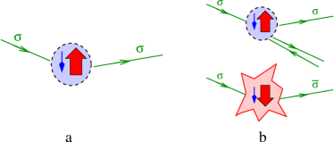
Figure 1: Sketch of (a) elastic and (b) inelastic scattering processes. In case of an inelastic scattering the outgoing electron leaves spin- and/or electron-hole excitations behind.

For quantum impurities in a free electron gas it is more transparent to introduce angular momentum channels, $L\equiv(l,m)$, and define the scattering states in terms of radially propagating states $|{\bf p},\sigma\rangle\to||{\bf p}|,L,\sigma\rangle$:

$$|{\bf p},\sigma\rangle=\sqrt{\frac{2}{\varrho}}\sum_{L}\int d\Omega_{\hat{p}}Y_{L}({\hat{p}})||{\bf p}|,L,\sigma\rangle\;,$$ (8)

with $Y_{L}({\hat{p}})$ the spherical functions, and $\varrho=\varrho(|{\bf p}|)$ the density of states of the conduction electrons. In this basis the on-shell $S$ and $T$-matrices become matrices in the angular momentum quantum numbers that depend only on the energy $\omega\equiv\xi({\bf p},\sigma)$ of the incoming particle. The $S$-matrix can then be expanded as

$$\langle{\bf p}\sigma|{\cal S}|{\bf p}^{\prime}\sigma^{\prime}\rangle={\frac{2}{\varrho}}\sum_{L,L^{\prime}}Y^{*}_{L}({\hat{\bf p}})\;s_{L\sigma,L^{\prime}\sigma^{\prime}}(\omega)\;Y_{L^{\prime}}({\hat{\bf p}}^{\prime})\;,$$ (9)

and the on-shell $T$-matrix is given by a similar expression, the coefficients of the expansions being related by

$${s}_{L,\sigma;\;L^{\prime}\sigma^{\prime}}(\omega)=\delta_{L,L^{\prime}}\delta_{\sigma,\sigma^{\prime}}+i\;{t}_{L,\sigma;\;L^{\prime}\sigma^{\prime}}(\omega)\;.$$ (10)

The eigenvalues ${\cal S}_{\lambda}$ of the matrix $s_{L,\sigma;\;L^{\prime}\sigma^{\prime}}$ must all be within the complex unit circle for any $\omega$, and they are directly related to the inelastic scattering cross section. To see this, let us consider the case of scattering only in the $s$-channel ($L=0$), and assume spin conservation. In this case $s_{L,\sigma;\;L^{\prime}\sigma^{\prime}}$ becomes a simple number, $s(\omega)=1+it(\omega)$,

$$s(\omega)=2\pi\varrho\;\langle{\bf p}\sigma|{\cal S}|{\bf p}^{\prime}\sigma^{\prime}\rangle=2\pi\varrho\;\;{\cal S}(\omega)$$

and the inelastic scattering cross section can be expressed as

$$\sigma_{\rm inel}(\omega) = \frac{\pi}{p_{F}^{2}}\;(1-|{s}(\omega)|^{2})$$ (11)

$$= \frac{\pi}{p_{F}^{2}}\;(2\;{\rm Im}\;t(\omega)-|t(\omega)|^{2})\;,$$

where we assumed free electrons of dispersion $\xi={\bf p}^{2}/2m-\mu$ with a Fermi energy $\mu$ and a corresponding Fermi momentum $p_{F}$. Eq. (11) implies that the scattering becomes totally elastic whenever ${s}(\omega)$ is on the unit circle, and it is maximally inelastic if the corresponding single particle matrix element of the $S$-matrix vanishes. The former situation occurs at Fermi liquid fixed points, while the latter case is realized, e.g., in the two-channel Kondo model or the two-impurity Kondo model. The total scattering cross section, on the other hand, is related to the real part of ${s}(\omega)$ as

$$\sigma_{\rm tot}(\omega)=\frac{2\pi}{p_{F}^{2}}\;(1-{\rm Re}\{{s}(\omega)\})=\frac{2\pi}{p_{F}^{2}}\;{\rm Im}\;t(\omega)\;.$$ (12)

It is easy to generalize this result to the case of many scattering channels, and one finds that inelastic scattering can take place only if some of the eigenvalues of $s_{L,\sigma;\;L^{\prime}\sigma^{\prime}}$ are not on the unit circle. singular

To compute the off-diagonal matrix element $\langle{\bf p}\sigma|{\cal T}|{\bf p}^{\prime}\sigma^{\prime}\rangle\;,$ we first relate it to the conduction electrons’ Green function through the so-called reduction formula detailed in Section II, Itzykson80

$$\langle{\bf p},\sigma|{\cal T}|{\bf p}^{\prime}\sigma^{\prime}\rangle=$$ (13)

$$-\;[G^{0}]^{-1}_{\pm{\bf p},\pm\sigma}(\xi)\;G_{\pm{\bf p}\;\pm\sigma,\pm{\bf p}^{\prime}\;\pm\sigma^{\prime}}(\xi)\;[G^{0}]^{-1}_{\pm{\bf p}^{\prime}\pm\sigma^{\prime}}(\xi)\;.$$

Here the $\pm$ signs correspond to electron and hole states with $\xi>0$ and $\xi<0$ and of energy $E=|\xi|$, $G_{0}$ denotes the free electron Green’s function, and $G$ the full many-body time-ordered electron Green’s function. Thus the positive frequency part of the Green’s function describes the scattering of electrons, while the negative frequency part that of holes. Strictly speaking, our derivation of this formula only holds for Fermi liquids, i.e., for models where the ground state has no internal degeneracy and can continuously be related to a non-interacting ground state. The consideration of internal ground state degeneracy needs some care, and the definition of inelastic scattering in that case is not straightforward. singular However, the finite temperature results of Ref. Rosch, show that Eqs. (5), (6), and (7) together with (13) provide the physically meaningful definition even in this case at $T=0$.

According to Eq. (13), to compute the inelastic and elastic scattering cross-sections, we need to evaluate the self-energy of the conduction electron’s Green function. We do this by relating the self-energy to some local correlation function, that we then compute either analytically within some approximation, or numerically using the powerful machinery of numerical renormalization group (NRG). NRG_ref This step depends on the specific impurity model at hand, and can be achieved through equation of motion methods, Costi diagrammatically, zar_inel or through a straightforward path integral treatment, as we do it in Section III. The recently-formulated scattering Bethe ansatz approach can possibly provide a way to avoid this numerical computation, and determine the full energy-dependence of the $S$-matrix analytically mehta .

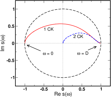
Figure 2: Renormalization group flow of the eigenvalues of the single particle $S$-matrix for the single- and two-channel Kondo models. For the single-channel Kondo model the scattering becomes elastic ($|S|=1$) both in the limit of very large and very small energies, $\omega\to\infty$, and $\omega\to 0$, respectively. For the 2-channel Kondo model ${s}(\omega\to 0)=0$, implying that half of the scattering remains inelastic even for $\omega\to 0$.

Let us close this Introduction by illustrating the power of this formalism through the simple examples of the single- and two-channel Kondo models, defined through the Hamiltonian:

$$H = \sum_{\alpha=1}^{f}\sum_{{\bf p},\sigma}\xi_{\bf p}\;a^{\dagger}_{{\bf p}\sigma,\alpha}a_{{\bf p}\sigma,\alpha}$$ (14)

$$+ \frac{J}{2}\vec{S}\sum_{\alpha=1}^{f}\sum_{\genfrac{}{}{0.0pt}{}{{\bf p},{\bf p}^{\prime}}{\sigma\sigma^{\prime}}}a^{\dagger}_{{\bf p}\sigma,\alpha}{\vec{\sigma}}_{\sigma\sigma^{\prime}}a_{{\bf p}^{\prime}\sigma^{\prime},\alpha}\;.$$

Here $a^{\dagger}_{{\bf p}\sigma\alpha}$ creates a conduction electron with momentum $\bf p$, spin $\sigma$ in channel $\alpha$, $S=1/2$ is the impurity spin, and $f=1$ and $f=2$ for the single- and two-channel Kondo models, respectively.

In both models the $T$-matrix can be related to the Green’s function of the so-called composite Fermion operator, $F_{\sigma\alpha}\equiv\sum_{\sigma^{\prime},{\bf p}}{\vec{S}}\cdot{\vec{\sigma}}_{\sigma\sigma^{\prime}}a_{{\bf p}\sigma^{\prime}\;\alpha}$, Costi which can then be computed using NRG. NRG_ref The evolution of the eigenvalue of the numerically obtained $S$-matrix is shown in Fig. 2. In both cases, ${s}(\omega)={s}(\omega/T_{K})$ is a universal function that depends only on the ratio $\omega/T_{K}$, with $T_{K}$ the so-called Kondo temperature, $T_{K}\approx E_{F}\;e^{-1/\varrho J}$, with $E_{F}$ the Fermi energy and $\varrho$ the density of states at the Fermi energy for one spin direction. Hewson ; Cox_Zawa

For the single-channel Kondo model the scattering becomes elastic both in the limit of very large and very small energies, $\omega\gg T_{K}$, and $\omega\ll T_{K}$, respectively, where the eigenvalues lie on the unit circle. The reasons are different: At large energies conduction electrons do not interact with the impurity spin efficiently. At very small energies, on the other hand, the impurity’s spin is screened and disappears from the problem apart from a residual phase shift of $\pi/2$ and an irrelevant local electron-electron interaction. Nozieres The maximum inelastic scattering is reached when the eigenvalue ${s}(\omega)$ is closest to the origin, i.e., at energies in the range of the Kondo temperature, $\omega\approx T_{K}$.

For the 2-channel Kondo model, on the other hand, ${s}(\omega\to 0)=0$, implying that the scattering is maximally inelastic even at the Fermi energy, $\omega\to 0$. This property of the $S$-matrix has been first noticed by Maldacena and LudwigMaldacena , and is characteristic of a non-Fermi liquid, where incoming electrons do not scatter into an outgoing single electron state, even at the Fermi energy. Note, however, that the vanishing of the $S$-matrix does not imply that all the scattering is fully inelastic. In fact, from Eqs. (5) and (6) it follows that

$$\sigma_{\rm inel}^{\rm 2CK}=\sigma_{\rm el}^{\rm 2CK}=\frac{\sigma_{\rm tot}^{\rm 2CK}}{2}\;,$$

i.e., half of the scattering remains still elastic. In other words, in the elastic channel, the unscattered and scattered $s$-electron wave functions are completely out of phase, and therefore there is no net outgoing particle in the $s$-channel.

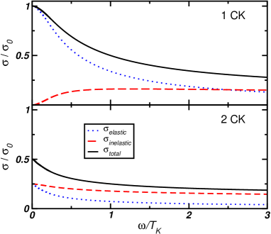
Figure 3: Top: Inelastic, elastic, and total scattering rates for the single-channel Kondo model in units of $\sigma_{0}=4\pi/p_{F}^{2}$ for a spin up electron. $\sigma_{\rm inel}$ scales approximately linearly with $\omega$ for $0.05\;T_{K}<\omega<0.5\;T_{K}$, behaves as $\sim\omega^{2}$ for $\omega<0.05\;T_{K}$, and remarkably, shows a plateau above $T_{K}$. Bottom: Same for the two-channel Kondo problem for a spin up electron in channel 1. Note that the inelastic scattering cross section remains finite at $\omega=0$, and is precisely half of the elastic scattering cross section.

The structure of the flow of ${s}(\omega)$ appears more directly in the in the energy dependence of the various scattering cross-sections shown in Fig. 3 for these two cases. In the single-channel case, it is quite remarkable that the low-energy $\sim\omega^{2}$ inelastic scattering cross section expected from Fermi liquid considerationsNozieres is limited only to the regime $\omega<0.05\;T_{K}$, and for $0.05\;T_{K}<\omega<0.5\;T_{K}$ the inelastic scattering cross section is quasi-linear. Furthermore, above $T_{K}$ a wide plateau appears (rather then a peak), where $\sigma(\omega)$ is large and almost independent of the energy $\omega$ of the incoming particle. Both features appear also in a finite temperature calculation, Rosch are in quantitative agreement with the experimental results of Refs. Saminadayar2006, ; mohanty2003, on magnetically doped wires, and provide a possible explanation of the observed saturation of the dephasing time in some experiments on dephasing Mohanty-Webb . As we show in Section VI, these universal features are robust and present in the Anderson model too.

It is important to emphasize here that in the present paper we computed the inelastic scattering rate of electrons, rather than that of quasiparticles. This is motivated by the trivial observation that in a real experiment, the external electromagnetic field couples with a minimal coupling to the bare conduction electrons. Precisely for this reason, the Kubo formula contains the conduction electron current operators, and also, the relevant quantity to determine dephasing is thus the inelastic scattering rate of electrons. This is what we have computed here and that has been computed in Refs. zar_inel and Rosch .

The definition of quasiparticles depends on the context in which they emerge. If one defines them as stable elementary excitations of the vacuum, as Nozières did Nozieres , or as they appear in Bethe ansatz BA , then, by definition, these quasiparticles do not decay at all at $T=0$ and scatter only elastically Nozieres .

Such quasiparticles are, however, usually complicated objects in terms of conduction electrons. For this reason they are typically not minimally coupled to the gauge field, and therefore, the current operator in the Kubo formula is a very complicated many-body vertex in the language of quasiparticles. Excepting for $\omega=0$, a real conduction electron is composed of many such stable quasiparticles, and it decays inelastically even at $T=0$ temperature, even if quasiparticles do not. In the Kondo model, at the Fermi energy quasiparticle states are simple phase shifted conduction electron states. However, the connection between quasiparticles and conduction electrons is not trivial for any finite energy. Therefore, if one considers inelastic scattering at a finite energy, one must precisely specify how finite energy quasiparticle states are defined, how they couple to a gauge field, and how a finite energy electronic state is decomposed in terms of these quasiparticles. Unfortunately, except for the Bethe ansatz, we are not aware of any work which would provide this necessary connection in sufficient detail, and would go beyond a simple heuristic treatment (which might still give the correct result). In the present framework, we avoided this difficulty by formulating the problem in terms of electrons rather than quasiparticles.

The paper is organized as follows: In Section II we present the derivation of the reduction formulas. In Section III we determine the T-matrix for the Kondo model. In Sections IV, V, and VI we present results on the inelastic scattering rate for the single- and two-channel Kondo model and for the Anderson model, respectively. In Section VII the results are summarized. In the Appendix some details of the derivation of the T-matrix for the Anderson model is discussed.

II Reduction Formulas

II.1 Definition of scattering states in the Heisenberg picture

Although reduction formulas are often used in the literature in a heuristic way, apart from the derivation of Langreth for the Anderson model, langreth we do not know of any work that would establish a rigorous connection between the single-particle matrix elements of the $T$-matrix and the conduction electron’s Green’s function for a general quantum impurity problem. Here we therefore present a short derivation of the reduction formulas by generalizing the procedure used in the domain of particle physics. Itzykson80 ; LeBellac

In this section, following the field theoretical language, we shall use the Heisenberg picture, and describe scattering in terms of the field operators, Itzykson80 $\psi_{\sigma}(x)$, where we introduced the four-vector notation, $x\equiv(t,{\bf x})$. The evolution of this field operator is described by the time-dependent Hamiltonian, with the interactions switched on and off adiabatically with a rate $\delta\to 0$,

$$H\equiv H(t)=H_{0}+e^{-\delta|t|}H_{\rm int}\,.$$ (15)

Here $H_{0}$ denotes the non-interacting Hamiltonian,

$$H_{0}=\int d^{3}{\bf x}\;\psi^{\dagger}_{\sigma}(x)[-\frac{\Delta}{2m}-\mu]\psi_{\sigma}(x),$$ (16)

with $\Delta$ the Laplace operator, and $\mu$ the chemical potential of the electrons. The interaction part $H_{\rm int}$ does not need to be specified at this point, and depends on the particular model considered. For the sake of simplicity we assume that the quantum impurity interacts with free electrons, but the procedure described can be generalized for electrons with more complicated dispersions, too.

Within the Heisenberg picture, states are independent of time, and all non-trivial scattering is incorporated in the time evolution of the fields. Scattering states can be defined through the asymptotic form of the field operators. Incoming and outgoing scattering states can be defined based on the simple observation that for times $t\to\pm\infty$ the equation of motion of $\psi_{\sigma}(x)$ is generated by $H_{0}$, and therefore $\psi_{\sigma}(x)$ behaves asymptotically as a free field:

$$\psi_{\sigma}(x,t\to-\infty)\to\int\frac{d^{3}\bf p}{(2\pi)^{3}}\,e^{-i\,p\cdot x}a_{p\,\sigma,\textrm{in}}\,,$$ (17)

where $a_{p\,\sigma,\textrm{in}}\equiv a_{{\bf p}\,\sigma,\textrm{in}}$ are just the annihilation operators of incoming (one particle) scattering states. Here for the sake of compactness, we introduced the four-momentum, $p\equiv(\xi,{\bf p})$, with $\xi=\xi({\bf p})={\bf p}^{2}/2m-\mu$ the energy of the conduction electrons, measured from the Fermi energy, and $p\cdot x=\xi\;t-{\bf p}\;{\bf x}$. The operators $a_{p\,\sigma,\textrm{in}}\equiv a_{{\bf p}\,\sigma,\textrm{in}}$ satisfy standard anti-commutation relations:

$$\{a_{p\,\sigma,\textrm{in}},a^{\dagger}_{p^{\prime}\,\sigma^{\prime},\textrm{in}}\}=(2\pi)^{3}\;\delta_{\sigma,\sigma^{\prime}}\;\delta({\bf p}-{\bf p}^{\prime})\;.$$ (18)

Note that the operators $a^{\dagger}_{p\,\sigma,\textrm{in}}$ do not create free electrons, rather, they are creation operators of incoming electrons in scattering states, which are asymptotically free.

The operators $a^{\dagger}_{p\,\sigma,\textrm{in}}$ can be used to construct incoming single particle scattering states, $|{\bf p},\sigma\rangle_{\textrm{in}}$. For electrons, i.e., excitations of momenta larger than the Fermi momentum, $|{\bf p}|>p_{F}$, these scattering states can be simply defined as

$$|{\bf p},\sigma\rangle_{\textrm{in}}\equiv a^{\dagger}_{p,\sigma,\textrm{in}}|0\rangle=\lim_{t\to-\infty}\int\textrm{d}^{3}{{\bf x}}\;e^{-ip\cdot x}\;\psi^{\dagger}_{\sigma}(x)|0\rangle\;.$$ (19)

Outgoing single electron scattering states, $|p,\sigma\rangle_{\textrm{out}}\equiv|{\bf p},\sigma\rangle_{\textrm{out}}$, can be defined in a similar way, by expanding the field $\psi_{\sigma}(x,t\to+\infty)$,

$$|{\bf p},\sigma\rangle_{\textrm{out}}\equiv a^{\dagger}_{p,\sigma,\textrm{out}}|0\rangle=\lim_{t\to+\infty}\int\textrm{d}^{3}{{\bf x}}\;e^{-ip\cdot x}\;\psi^{\dagger}_{\sigma}(x)|0\rangle\;.$$ (20)

Incoming and outgoing hole states must be defined slightly differently, because an incoming hole of energy $E>0$, momentum ${\bf p}$, and spin $\sigma$ is created by removing an electron of energy $\xi=-E$, momentum $-{\bf p}$, and spin $-\sigma$ from the Fermi surface. In other words, incoming hole scattering states are defined for $|{\bf p}|<p_{F}$ as

$$|{\bf p},\sigma\rangle_{\textrm{in/out}}\equiv a_{-p,-\sigma,\textrm{in/out}}|0\rangle$$ (21)

$$\phantom{aa}=\lim_{t\to\mp\infty}\int\textrm{d}^{3}{{\bf x}}\;e^{-ip\cdot x}\;\psi_{-\sigma}(x)|0\rangle\;\phantom{aaaa}(|{\bf p}|<p_{F})\;.$$

II.2 Reduction formulas and Green’s functions

We proceed to derive a general relation involving Green’s functions to express the off-diagonal matrix elements

$$i\;\langle{\bf p}\;\sigma|\hat{T}|{\bf p}^{\prime}\sigma^{\prime}\rangle=\phantom{a}_{\textrm{out}}\langle{\bf p}\;\sigma|{\bf p}^{\prime}\;\sigma^{\prime}\rangle_{\textrm{in}}\quad\quad({\bf p}\neq{\bf p}^{\prime})$$ (22)

for electronic excitations with $|{\bf p}|>p_{F}$ first. Using the asymptotic expression Eq. (19) this matrix element can be expressed as

$$\phantom{a}{}_{\textrm{out}}\langle{\bf p}\;\sigma|{\bf p}^{\prime}\;\sigma^{\prime}\rangle_{\textrm{in}} =$$ (23)

$$\lim_{y_{0}\to-\infty}\phantom{a}{}_{\textrm{out}}\langle{\bf p},\sigma|\int_{y_{0}}\textrm{d}^{3}{\bf y}\;e^{-ip^{\prime}y}\psi^{\dagger}_{\sigma^{\prime}}(y)|0\rangle\;.$$

Integrating by part we obtain

$$\lim_{y_{0}\to-\infty}\int_{y_{0}}\textrm{d}^{3}{\bf y}\;e^{-ip^{\prime}y}\psi^{\dagger}_{\sigma^{\prime}}(y)=$$

$$= -\int\textrm{d}^{4}y\frac{\partial}{\partial y_{0}}\left[e^{-ip^{\prime}y}\psi^{\dagger}_{\sigma^{\prime}}(y)\right]+a^{\dagger}_{p^{\prime},\sigma^{\prime},\textrm{out}}.$$

The last term does not give a contribution to the matrix element for $p\neq p^{\prime}$, therefore we drop it. The rest can be expressed as

$$\int_{-\infty}^{\infty}\textrm{d}^{4}y\frac{\partial}{\partial y_{0}}\left[e^{-ip^{\prime}y}\psi^{\dagger}_{\sigma^{\prime}}(y)\right]=$$

$$-i\int\textrm{d}^{4}ye^{-ip^{\prime}y}\left[i\frac{\partial}{\partial y_{0}}+H_{0}({\bf y})\right]\psi^{\dagger}_{\sigma^{\prime}}(y),$$

where we obtained the r.h.s. of this equation by using the fact that $p^{\prime}$ is on the energy shell, and therefore $p_{0}^{\prime}e^{-ip^{\prime}y}=(-\frac{1}{2m}\Delta_{\bf y}-\mu)e^{-ip^{\prime}y}$, and then by integrating by part with respect to ${\bf y}$. Thus the off-diagonal matrix elements of the $S$-matrix simplify to

$$\phantom{a}{}_{\textrm{out}}\langle{\bf p}\;\sigma|{\bf p}^{\prime}\;\sigma^{\prime}\rangle_{\textrm{in}}=$$ (24)

$$\phantom{aaaa}i\int\textrm{d}^{4}ye^{-ip^{\prime}y}\left[i\frac{\partial}{\partial y_{0}}+H_{0}({\bf y})\right]\phantom{a}_{\textrm{out}}\langle{\bf p}\sigma|\psi^{\dagger}_{\sigma^{\prime}}(y)|0\rangle$$

Using the asymptotic relation of the outgoing states, (20), we can now write the full matrix element as

$$\phantom{a}{}_{\textrm{out}}\langle{\bf p}\;\sigma|{\bf p}^{\prime}\;\sigma^{\prime}\rangle_{\textrm{in}}=i\int\textrm{d}^{4}ye^{-ip^{\prime}y}\left[i\frac{\partial}{\partial y_{0}}+H_{0}({\bf y})\right]\times$$ (25)

$$\times \lim_{x_{0}\to\infty}\int\textrm{d}^{3}{\bf x}\;e^{ipx}\langle 0|\psi^{\phantom{\dagger}}_{\sigma}(x)\psi^{\dagger}_{\sigma^{\prime}}(y)|0\rangle.$$

Once again, we convert the last integral into an integral over the whole space-time, which yields

$$\lim_{x_{0}\to\infty}\int\textrm{d}^{3}{\bf x}\;e^{ipx}\langle 0|\psi^{\phantom{\dagger}}_{\sigma}(x)\psi^{\dagger}_{\sigma^{\prime}}(y)|0\rangle$$ (26)

$$= \int^{\infty}_{-\infty}\textrm{d}^{4}{x}\frac{\partial}{\partial x_{0}}e^{ipx}\langle 0|T\psi^{\phantom{\dagger}}_{\sigma}(x)\psi^{\dagger}_{\sigma^{\prime}}(y)|0\rangle$$

where the time ordering operator $T$ has been inserted to assure that the $x_{0}\to-\infty$ contribution vanishes by Eq. (19): $\lim_{x_{0}\to-\infty}\int\textrm{d}^{3}{\bf x}\;e^{ipx}\langle 0|\psi^{\dagger}_{\sigma^{\prime}}(y)\psi^{\phantom{\dagger}}_{\sigma}(x)|0\rangle=0$.

We can manipulate the remaining expression in the same way as before to finally obtain

$$\phantom{a}{}_{\textrm{out}}\langle{\bf p}\;\sigma|{\bf p}^{\prime}\;\sigma^{\prime}\rangle_{\textrm{in}}=-\int\textrm{d}^{4}x\;\textrm{d}^{4}y\;e^{-ip^{\prime}y}e^{ipx}\left[\left(-i\;\overrightarrow{\partial}_{x_{0}}-\vec{H}_{0}({\bf x})\right)\langle\textrm{T}\psi^{\phantom{\dagger}}_{\sigma}(x)\psi^{\dagger}_{\sigma^{\prime}}(y)\rangle\left(i\;\overleftarrow{\partial}_{y_{0}}-H_{0}({\bf y})\right)\right]\;,$$ (27)

where the arrows indicate forward and backward differentiation, respectively. Observing that the operator $(-i\;{\partial}_{x_{0}}-H_{0}({\bf x}))\;\delta(x-x^{\prime})$ is simply the matrix element of the inverse of the non-interacting Green’s function,

$$\langle x^{\prime}|\hat{G}^{-1}_{0}|x\rangle = \delta(x^{\prime}-x)\;\left(-i\;\overrightarrow{\partial}_{x_{0}}-H_{0}({\bf x})\right)\;,$$

$$= \left(i\;\overleftarrow{\partial}_{{x}_{0}^{\prime}}-H_{0}({\bf x}^{\prime})\right)\;\delta(x^{\prime}-x)\;,$$

Eq. (27) can be simply expressed as

$$\phantom{a}{}_{\textrm{out}}\langle{\bf p}\;\sigma|{\bf p}^{\prime}\;\sigma^{\prime}\rangle_{\textrm{in}}=$$ (28)

$$\phantom{aaa}-i\int\textrm{d}^{4}x\;\textrm{d}^{4}y\;e^{ipx-ip^{\prime}y}\left[\hat{G}^{-1}_{0}\ast\hat{G}\ast\hat{G}^{-1}_{0}\right]_{x,y}\;,$$

with ’$\ast$’ the four-dimensional convolution operator, and $\hat{G}$ the usual interacting Green’s function,

$$G_{\sigma\sigma^{\prime}}(x,y)=-i\;\langle T\psi^{\phantom{\dagger}}_{\sigma}(x)\psi^{\dagger}_{\sigma^{\prime}}(y)\rangle\;.$$ (29)

The Fourier transformation of (28) then yields

$$\phantom{a}{}_{\textrm{out}}\langle{\bf p}\;\sigma|{\bf p}^{\prime}\;\sigma^{\prime}\rangle_{\textrm{in}}=$$ (30)

$$\phantom{a}-i\;G^{-1}_{0,\sigma}(p)G^{\phantom{1}}_{\sigma,\sigma^{\prime}}(p,p^{\prime})G^{-1}_{0,\sigma}(p^{\prime}).\phantom{aaaaaa}(|{\bf p}|>p_{F})$$

Translational invariance in time further implies

$$G^{\phantom{1}}_{\sigma,\sigma^{\prime}}(p,p^{\prime}) = \phantom{a}\;2\pi\;\delta(\xi({\bf p}^{\prime})-\xi({\bf p}))\;G^{\phantom{1}}_{{\bf p}\sigma,{\bf p}^{\prime}\sigma^{\prime}}(\xi({\bf p})).$$

Inserting this into (30) and comparing it with Eq. (4) yields Eq. (13) for $\xi>0$.

The derivation for holes follows exactly the same lines excepting that the matrix element to be computed is now

$$\phantom{a}{}_{\textrm{out}}\langle{\bf p}\;\sigma|{\bf p}^{\prime}\;\sigma^{\prime}\rangle_{\textrm{in}}=\langle 0|a^{\dagger}_{-p,-\sigma,\textrm{out}}a^{\phantom{\dagger}}_{-p^{\prime},-\sigma^{\prime},\textrm{in}}|0\rangle,$$ (31)

and correspondingly, the final expression of the $S$-matrix element now reads for ${\bf p}\neq{\bf p}^{\prime}$

$$\phantom{a}{}_{\textrm{out}}\langle{\bf p}\;\sigma|{\bf p}^{\prime}\;\sigma^{\prime}\rangle_{\textrm{in}}=\phantom{aaaaaaaaaaaaaaaaaa}(|{\bf p}|<p_{F})$$

$$\phantom{aaaa}i\;G^{-1}_{0,-\sigma^{\prime}}(-p^{\prime})G^{\phantom{1}}_{-\sigma^{\prime},-\sigma}(-p^{\prime},-p)G^{-1}_{0,-\sigma}(-p)\;.$$

III T-matrix of the Kondo model

For practical calculations, one needs to determine the $T$-matrix of Eq. (13) somehow. For most really interesting cases this can be done analytically only approximately and in a limited energy range, and numerical methods must be used. The most adequate way to perform the calculation is to first relate the $T$-matrix to some local correlation function that can then be computed using Wilson’s numerical renormalization group method. NRG_ref To establish the desired relation, one can use equation of motion methods, Costi or do diagrammatic perturbation theory and sum up the diagrams up to infinite order, zar_inel but here we show yet another rather elegant way, in terms of path integrals.

Although this method works for essentially any quantum impurity problem, here we show how it works for the Kondo model, already defined in the introduction (see Eq. (14)). The application of this method to the Anderson model is discussed in the Appendix. To use a field theoretical formalism, following Abrikosov, we represent the impurity spin $\vec{S}$ by fermionic operators, $f_{\sigma}$,

$$\vec{S}=\frac{1}{2}\sum_{\sigma,\sigma^{\prime}}f^{\dagger}_{\sigma}\vec{\sigma}_{\sigma\sigma^{\prime}}f^{\phantom{\dagger}}_{\sigma^{\prime}}\;,\phantom{nnn}\sum_{\sigma}f^{\dagger}_{\sigma}f^{\phantom{\dagger}}_{\sigma}\equiv 1\;.$$ (32)

Next, we define the generating functional for the conduction electron Green’s functions as follows:

$$Z[\eta_{\sigma},\overline{\eta}_{\sigma}]=\int D\left[a_{\sigma}\overline{a}_{\sigma}\right]\tilde{D}\left[f_{\sigma}\overline{f}_{\sigma}\right]e^{-i\;S}e^{i\overline{\eta}\cdot a+i\overline{a}\cdot{\eta}},$$ (33)

where the tilde on the second integration measure indicates that one must impose the constraint $\sum_{\sigma}f^{\dagger}_{\sigma}f^{\phantom{\dagger}}_{\sigma}\equiv 1$ when performing the path integral, and we introduced the shorthand notation: $\overline{\eta}\cdot a\equiv\sum_{{\bf p},\sigma}\int dt\;\overline{\eta}_{{\bf p},\sigma}(t)a_{{\bf p},\sigma}(t)\;.$ The action $S$ in Eq. (33) consists of three terms, $S=S_{e}+S_{f}+S_{\rm int}$: The first term, $S_{e}$ describes the conduction electrons,

$$S_{e}=-\sum_{{\bf p},\sigma}\int dt\;dt^{\prime}\;\overline{a}_{{\bf p}\sigma}(t)[G^{0}]^{-1}_{{\bf p}}(t-t^{\prime})\;a_{{\bf p}\sigma}(t^{\prime})$$ (34)

with $G^{0}$ the time-ordered free electron Green’s function. The term $S_{f}\equiv-i\;\sum_{\sigma}\int dt\;\overline{f}_{\sigma}(t)\;\frac{d}{dt}f_{\sigma}(t)$ generates the spin dynamics, while the last term simply describes the interaction:

$$S_{\rm int}\equiv\frac{J}{2}\;\sum_{\genfrac{}{}{0.0pt}{}{{\bf p},{\bf p}^{\prime}}{\sigma,\sigma^{\prime}}}\int dt\;\vec{S}(t)\;\overline{a}_{{\bf p}\sigma}(t)\vec{\sigma}_{\sigma\sigma^{\prime}}a_{{\bf p}^{\prime}\sigma^{\prime}}(t)\;.$$ (35)

The full time-ordered Green’s function is related to $Z$ by

$$G_{{\bf p}\sigma,{\bf p}^{\prime}\sigma^{\prime}}(t-t^{\prime})=\left.\frac{1}{i}{\frac{\delta^{2}\textrm{ln}Z[\overline{\eta},\eta]}{\delta\overline{\eta}_{{\bf p}\sigma}(t)\delta\eta_{{\bf p}^{\prime}\sigma^{\prime}}(t^{\prime})}}\right|_{\eta=\overline{\eta}=0}\;.$$ (36)

We can derive the required identity by simply shifting the integration variable in Eq. (33),

$$a_{{\bf p}\sigma}(t)\to a_{{\bf p}\sigma}(t)-\int dt^{\prime}\;G^{0}_{{\bf p}}(t-t^{\prime})\;\eta_{{\bf p}\sigma}(t^{\prime})\;.$$ (37)

As a result, the exponent in Eq. (33) transforms to:

$$S-\overline{\eta}\cdot a-\overline{a}\cdot{\eta}\phantom{a}\Rightarrow\phantom{a}S + \sum_{{\bf p},\sigma}\int dt\;dt^{\prime}\;\overline{\eta}_{{\bf p}\sigma}(t)G^{0}_{{\bf p}\sigma}(t-t^{\prime})\eta_{{\bf p}\sigma}(t^{\prime})\;-\frac{J}{2}\sum_{{\bf p},\sigma}\int dt\;dt^{\prime}\;\left(\overline{F}_{\sigma}(t)G^{0}_{{\bf p}\sigma}(t-t^{\prime})\eta_{{\bf p}\sigma}(t^{\prime})\;+{\rm h.c.}\right)$$

$$+\frac{J}{2}\;\sum_{\genfrac{}{}{0.0pt}{}{{\bf p},{\bf p}^{\prime}}{\sigma,\sigma^{\prime}}}\int dt\;dt^{\prime}\;dt^{\prime\prime}\;\overline{\eta}_{{\bf p}\sigma}(t)G^{0}_{{\bf p}\sigma}(t-t^{\prime})\vec{S}(t^{\prime})\vec{\sigma}_{\sigma\sigma^{\prime}}G^{0}_{{\bf p}\sigma}(t^{\prime}-t^{\prime\prime})\eta_{{\bf p}^{\prime}\sigma}(t^{\prime\prime})\;,$$

where we introduced the composite fermion field, $F_{\sigma}(t)\equiv\sum_{{\bf p},\sigma^{\prime}}\vec{S}(t)\vec{\sigma}_{\sigma\sigma^{\prime}}a_{{\bf p},\sigma^{\prime}}(t)$. Carrying now out the functional derivation of (36) we obtain the following simple relation

$$G_{{\bf p}\sigma,{\bf p}^{\prime}\sigma^{\prime}}(t-t^{\prime})=\delta_{{\bf p},{\bf p}^{\prime}}\;G^{0}_{{\bf p}\sigma}(t-t^{\prime})+\int d\tilde{t}\;d\tilde{t}^{\prime}\;G^{0}_{{\bf p}\sigma}(t-\tilde{t})\left(\delta(\tilde{t}-\tilde{t}^{\prime})\;\frac{J}{2}\langle\vec{S}\rangle\vec{\sigma}_{\sigma\sigma^{\prime}}-i\;\frac{J^{2}}{4}\langle F_{\sigma}(\tilde{t})\overline{F}_{\sigma^{\prime}}(\tilde{t}^{\prime})\rangle\right)G^{0}_{{\bf p}^{\prime}\sigma^{\prime}}(\tilde{t}^{\prime}-t^{\prime}).$$ (38)

The average in this expression must be carried out by computing the appropriate path integral, and results in the corresponding time-ordered Green’s function. Comparing Eqs. (38) and (13), and using the analytical properties of the time-ordered and retarded Green’s functions at $T=0$ temperature, we finally obtain the relations:

$${\rm Im}\{{\cal T}_{\tau\sigma,\tau\sigma^{\prime}}(\omega)\} = \pi\frac{J^{2}}{4}\varrho_{F,\sigma\sigma^{\prime}}(\omega)\;,$$ (39)

$$-\tau\ {\rm Re}\{{\cal T}_{\tau\sigma,\tau\sigma^{\prime}}(\omega)\} = \frac{J}{2}\langle\vec{S}\rangle\vec{\sigma}_{\sigma\sigma^{\prime}}+\frac{J^{2}}{4}\;{\cal P}\int d\omega^{\prime}\;\frac{\varrho_{F,\sigma\sigma^{\prime}}(\omega)}{\omega-\omega^{\prime}}\;,$$

with $\varrho_{F,\sigma\sigma^{\prime}}(\omega)$ the spectral function of the composite Fermion’s Green function, and $\tau={\rm sgn}\;\xi$. Note that scattering takes place only in the $s$-channel, and therefore these matrix elements do not depend on the incoming and outgoing momenta of the excitations. Eqs. (38) and (39) can be easily visualized in terms of diagrammatic perturbation theory, as shown in Fig. 4. The spectral function appearing in Eq. (39) is just a local correlation function that can be easily obtained through the NRG method. NRG_ref In the following sections we shall primarily use this method to compute the single particle $T$-matrix and the inelastic scattering rates of the basic quantum impurity models, the single-channel Kondo model, the two-channel Kondo model, and the Anderson model. Calculations for the spin $S=1$ Anderson model have been performed in Ref. Hewson2,

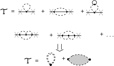
Figure 4: Diagrammatic representation of the $T$-matrix in the Kondo problem. Dashed lines denote pseudo-fermion propagators and describe the evolution of the impurity spin, while continuous lines denote free conduction electron propagators. Filled circles stand for the exchange interaction $J$. The first term of the $T$-matrix is simply proportional to the expectation value of the impurity spin, it is frequency independent, and vanishes in the absence of magnetic field. The second term can be identified as the composite fermions correlation function.

IV Inelastic scattering in the Kondo model

In the previous sections we have related the single particle $T$-matrix and therefore the elastic and inelastic scattering amplitude of electrons with local correlation functions through the reduction formulas. In this section we shall use these results to analyze the $T=0$ temperature scattering properties of the Kondo model using Wilson’s NRGNRG_ref . However, before presenting detailed numerical results, let us shortly discuss what one can learn from simple perturbation theory.

Let us discuss the high-energy scattering of conduction electrons in the absence of external magnetic field. In this limit one can attempt to do perturbation theory, and in first non-vanishing order one obtains

$$t(\omega)=i\;2\pi\varrho\;{\cal T}(\omega)=-i\frac{\pi^{2}}{2}\;\;S(S+1)\;j^{2}+\dots\;,$$ (40)

where the dimensionless coupling $j=\varrho J$ has been introduced. Summing up the leading logarithmic diagrams amounts in replacing $J$ by the renormalized coupling, and gives

$$t(\omega\gg T_{K})\approx i\frac{\pi^{2}}{2}S(S+1)\frac{1}{\ln^{2}(\omega/T_{K})}\;,$$

with $T_{K}\sim E_{F}e^{-1/J\varrho}$ the Kondo temperature. Thus, in leading logarithmic order, the total scattering cross section is given by:

$$\sigma_{\rm tot}(\omega\gg T_{K})\approx\frac{\pi^{3}}{p_{F}^{2}}\;S(S+1)\frac{1}{\ln^{2}(\omega/T_{K})}\;.$$

The first non-vanishing contribution to the elastic scattering cross section, on the other hand, scales as $\sigma_{\rm el}\sim|t|^{2}\sim j^{4}$, and therefore $\sigma_{\rm el}(\omega)$ asymptotically behaves as

$$\sigma_{\rm el}(\omega\gg T_{K})\approx\frac{\pi^{5}}{4\;p_{F}^{2}}\;S^{2}(S+1)^{2}\frac{1}{\ln^{4}(\omega/T_{K})}\;.$$

This implies that asymptotically, all the scattering is inelastic

$$\sigma_{\rm inel}(\omega\gg T_{K})\approx\sigma_{\rm tot}(\omega)\approx\frac{\pi^{3}}{p_{F}^{2}}\;S(S+1)\frac{1}{\ln^{2}(\omega/T_{K})}\;.$$ (41)

This is a very surprising result, and contradicts to the conventional wisdom, which tries to associate inelastic scattering with spin-flip scattering from a free spin. In fact, this rather non-trivial result has been explained in Ref. Garst, in the following way: At high energies, incoming electrons are scattered by the impurity spin fluctuations. These fluctuations can absorb an energy of the order of $\sim T_{K}$, and therefore the energy of the incoming electron is not conserved in leading order, but it typically changes by a tiny amount, $\delta\omega\sim T_{K}$. In the most pedestrian perturbative approach this tiny energy transfer is neglected and therefore one concludes incorrectly that the energy is conserved in leading order.

We can also relate the cross sections above to scattering rates. Assuming a finite concentration $n_{\rm imp}$ of magnetic impurities, we can compute the impurity averaged conduction electron Green’s functions and from that the conduction electron lifetime:

$$\frac{1}{\tau}=n_{\rm imp}\;v_{F}\;\sigma_{\rm tot}(\omega)\approx n_{\rm imp}\frac{\pi S(S+1)}{2\;\varrho\;\ln^{2}(\omega/T_{K})}\;.$$ (42)

In fact, the first part of this equation gives a general rule to connect various cross sections to the corresponding scattering times, and for the inelastic scattering rate, e.g., we have

$$\frac{1}{\tau_{\rm inel}}=n_{\rm imp}\;v_{F}\;\sigma_{\rm inel}(\omega)\;.$$ (43)

For very large frequencies, again, the inelastic scattering rate is approximately equal to the elastic scattering rate:

$$\frac{1}{\tau_{\rm inel}}\approx n_{\rm imp}\frac{\pi S(S+1)}{2\;\varrho\;\ln^{2}(\omega/T_{K})}\;.$$ (44)

Note that this rate is a factor of 3/2 larger than the Nagaoka-Suhl expression, which only takes into account spin flip processes. Nagaoka

For energies $|\omega|\ll T_{K}$ perturbation theory breaks down, and it is more appropriate to use Nozieres’ Fermi liquid theory, which states that at the Fermi energy scattering is completely elastic, and Nozieres

$$t_{\sigma}(\omega=0^{+})=2\pi\varrho\;{\cal T}_{\sigma}^{1CK}(\omega=0^{+})=2\sin\delta_{\sigma}\;e^{i\delta_{\sigma}},$$ (45)

where we now allowed for a magnetic field pointing along the z-direction, and $\delta_{\sigma}$ stands for the phase shifts of electrons with spin $\sigma$ at the Fermi energy. Eq. (45) then yields

$$\sigma_{\rm tot,\sigma}(\omega\to 0)=\frac{4\pi}{p_{F}^{2}}\sin^{2}(\delta_{\sigma})\;,$$ (46)

$$\sigma_{\rm inel,\sigma}(\omega\to 0)=0\;.$$ (47)

The maximum total scattering cross section is reached in the unitary limit, $\delta_{\sigma}=\pi/2$.

Let us now proceed and compute the various scattering cross section using Wilson’s NRG NRG_ref . In the previous section, we showed how the imaginary part of the single particle $T$-matrix is related to composite Fermion’s spectral function, $\varrho_{F}(\omega)$. Within NRG, spectral functions of local operators are computed using their Lehman representation. The imaginary part of the $T$-matrix, related to the total scattering rate has already been computed in this way by Costi to obtain the magneto-resistivity of Kondo alloys. Costi To evaluate the inelastic scattering amplitude, however, one needs to go one step further and compute the real part of the $T$-matrix as well through a Hilbert transformation, Eq. (39). In such a calculation it is essential to have high quality data. The most challenging task is to obtain the correct $\sim\omega^{2}$ low energy behavior of the inelastic amplitude since we get this small quantity as a difference of two quantities of the order of unity. Therefore it is also crucial to get the normalization factor of $T$ correctly. In case of the single-channel Kondo problem this can be obtained through the Fermi liquid relation, (45): This relation connects the normalization of $t(\omega)$ to the phase shifts at the Fermi energy, which we extract from the NRG finite size spectrum very accuratelyHofstetter .

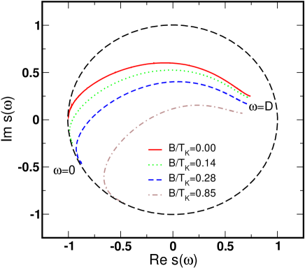
Figure 5: Renormalization group flow of the eigenvalues of the single particle $S$-matrix for the single-channel Kondo model in presence of a local magnetic field.

The renormalization group flow of the eigenvalues of the single particle $S$-matrix has already been shortly discussed in the introduction in the absence of magnetic fields (see Fig.1). The eigenvalues $s(\omega)$ of the $S$-matrix lie within the complex unit circle, and inelastic processes are allowed only when the eigenvalue $s(\omega)$ of the $S$-matrix satisfies $|s(\omega)|<1$. Incoming particles of high enough energy ($\omega\to\infty$) do not see the impurity, and therefore $s(\omega)\to 1$, corresponding to the weak coupling fixed point with phase shift $\delta\approx 0$. As expected for a Fermi liquids, at the Fermi energy ($\omega\to 0$) the $s(\omega)$ approaches the unit circle again, $s(\omega=0)=-1$, corresponding to the strong coupling fixed point of the Kondo model characterized by a phase shift $\delta=\pi/2$.

Application of a local magnetic field makes the flow more complicated (see Fig.5.): At low energy the system still behaves like a Fermi liquid but the position of the point where the $s(\omega)$ approaches the unit circle now varies with magnetic field. This is due to the magnetic field dependence of the scattering phase shifts at zero frequency.

For intermediate energy values of the incoming electron $|s(\omega)|<1$ and the inelastic scattering cross-section is non-zero. The total, elastic and inelastic scattering cross sections of an electron scattered off a magnetic impurity are shown in Fig.6. As expected, the inelastic amplitude always vanishes at the Fermi level. In the lower panel we show the inelastic scattering rate as compared to the Nagaoka-Suhl formula. The numerical results are consistent with the analytical expression (41) at large energies, while for energies much smaller than $T_{K}$ we recover the quadratically vanishing inelastic rate expected from Fermi liquid theory. NozieresII Note that the Nagaoka-Suhl approximation systematically underestimates the inelastic scattering rate by a factor of 2/3 since it considers any spin-diagonal process as elastic scattering. At high energies, however, in leading order all the scatterings are inelastic since even a spin diagonal process breaks up the Kondo singlet and leaves the system in an excited state, and therefore it cannot be elastic. Apart from this prefactor, the Nagaoka-Suhl result is perfect at high energies, however, it starts to deviate strongly from the numerically exact curve at approximately $10T_{K}$, and it completely fails below the Kondo temperature $T_{K}$. At energies well above $T_{K}$ almost all the scattering is inelastic, i.e. the inelastic amplitude varies as $\sim\ln^{-2}(\omega/T_{K})$ while the elastic part vanishes faster as $\sim\ln^{-4}(\omega/T_{K})$, in agreement with the analytical results.

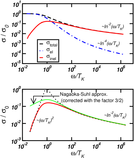
Figure 6: Upper panel: Inelastic, elastic, and total scattering rates for the single-channel Kondo model in units of $\sigma_{0}=4\pi/p_{F}^{2}$ at $T=0$ and $B=0$, as a function of the incoming electron’s energy. Only the electronic contribution ($\omega>0$) is plotted. For $\omega\gg T_{K}$ the inelastic rate as well as the total scattering rate varies as ${\rm ln}^{-2}(T_{K}/\omega)$ while the elastic part decays as ${\rm ln}^{-4}(T_{K}/\omega)$. The lower panel shows the $\sim\omega^{2}$ and ${\rm ln}^{-2}(T_{K}/\omega)$ regimes for $\omega\ll T_{K}$ and $\omega\gg T_{K}$, respectively. The Nagaoka-Suhl approximation, corrected with a factor $3/2$ (see the text) is also shown.

Even though the numerics recover the expected asymptotics, interesting features appear both in the low and high energy part of the scattering properties. First, as shown in Fig.3, the $\sigma_{\rm inel}\sim\omega^{2}$ regime appears only at energies well below the Kondo temperature, and we find that the inelastic scattering rate is roughly linear between $0.05T_{K}<\omega<0.5T_{K}$. Even though our calculation is done at $T=0$ temperature, we expect that $\sigma_{\rm inel}(T,\omega=0)$ behaves very similarly to $\sigma_{\rm inel}(T=0,\omega)$. Our results are thus consistent with the existing experimental data, explain the linear behavior observed in many experiments, mohanty2003 ; Saminadayar2003 ; Saminadayar2005 and surprisingly even quantitatively fit the finite temperature experimental curves. Saminadayar2005 Of course, in reality a finite temperature calculation is needed which has been performed in Ref. Rosch .

Another remarkable feature is the broad plateau in the inelastic scattering cross section above the Kondo scale, where the energy-dependence of the inelastic scattering rate turns out to be extremely weak. This weak energy-dependence provides a natural explanation for the experimentally observed plateau of the dephasing rate in many experiments. Mohanty-Webb ; Birge2003

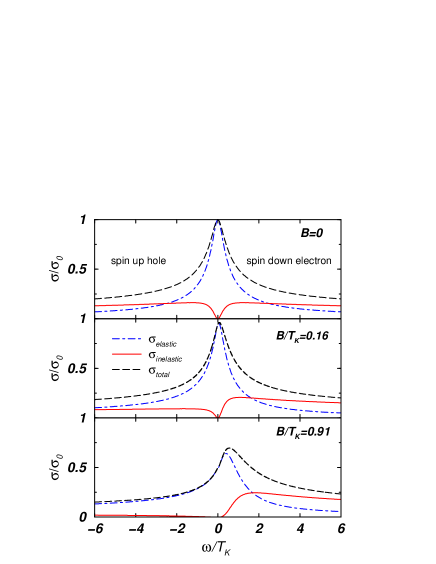
Figure 7: Energy dependence of spin-dependent elastic and inelastic scattering rates for the single-channel Kondo model in units of $\sigma_{0}=4\pi/p_{F}^{2}$, at $T=0$ and in the presence of a local magnetic field $B$. Note that the positive frequency side corresponds to spin down electrons, while the negative frequency side is for spin up holes. The impurity spin is polarized upwards.

The inelastic scattering amplitude in presence of a magnetic field is shown in Fig.7. Applying a local magnetic field breaks the spin symmetry of the scattering and changes the inelastic scattering properties of spin up and down particles dramatically. Already a relatively small magnetic field $B\sim 0.1T_{K}$ results in a very strong spin asymmetry of the inelastic scattering. For $B\sim T_{K}$ the effect is even more dramatic: At this field the impurity is practically polarized and aligned with the direction of the field and points upwards. As a result, an incoming spin up particle cannot flip the local spin in a first order process, and higher order processes are needed to generate inelastic scattering. A spin down electron or hole, on the other hand, can exchange its spin with the magnetic impurity, resulting in the maximum of the inelastic rate at energy $\approx B$ and a very broad inelastic background for $\omega>B$.

V Inelastic scattering in the two-channel Kondo model

In this section we shall present results for the two-channel Kondo model, the prototype of all non-Fermi liquid impurity models. AndreiDestrii ; AL In the channel symmetric case there is two types of conduction electrons that try to screen the impurity independently leading to the overscreening of the local moment. This frustration of the screening processes manifests itself in the formation of a strongly correlated state which cannot be described in the framework of Fermi liquid theory. This unusual correlated state manifests in the nonzero residual entropy, the logarithmic divergence of the impurity susceptibility and the power law behavior of transport properties with fractional exponents.

Since the non-Fermi liquid behavior is a direct consequence of the frustration of the screening processes, any infinitesimal asymmetry in the couplings $\Delta\equiv(j_{1}-j_{2})/(j_{1}+j_{2})$ leads to the appearance of another low temperature energy scale $T^{*}\propto\Delta^{2}/T_{K}$ at which the system crosses over to a Fermi liquid: Electrons being more strongly coupled to the impurity form a usual Kondo singlet with the impurity spin, while the other electron channel becomes completely decoupled from the spin.

In the 2-channel Kondo case, unfortunately, no Fermi-liquid relations similar to Eq. (45) are available. However, there is an exact theorem by Maldacena and Ludwig, that allows us to get the right normalization of the $T$-matrix. This theorem states that, at the two-channel Kondo fixed point, the single-particle elements of the $S$-matrix vanish at the Fermi energy, $s_{2CK}(\omega\to 0)=0$, Maldacena and as a consequence

$$t_{2CK}(\omega=0^{+})=-i\;.$$

This relation allows us to obtain the proper normalization of the numerically computed $T$-matrix even at the non-Fermi liquid fixed point. However, it also leads to the surprising result mentioned already in the introduction, that exactly half of the scattering is inelastic at the Fermi energy, while the other half of it is inelastic. This counter-intuitive result can be understood as follows: The identically zero single particle $S$-matrix indicates that an incoming electron cannot be detected as one electron after the scattering event, and it “decays” into many electron-hole pairs. To get such a “decay”, the scattering process must have an elastic component too which interferes destructively with the not scattered direct wave and results in the absence of the outgoing single particle amplitude in the $s$-channel.

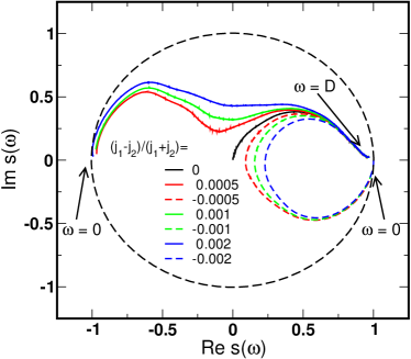
Figure 8: Renormalization group flow of the eigenvalues of the single particle $S$-matrix for the two-channel Kondo model for various values of channel asymmetry. The curves correspond to $j_{1}+j_{2}=0.12$.

The universal flow of the eigenvalue of the $S$-matrix was shown in Fig. 2. In Fig.8 we show what happens if we make the couplings in the two channels slightly asymmetric. For any small asymmetry the Fermi liquid behavior reappears: The $S$-matrix in the more strongly coupled channel flows first close to the two-channel Kondo fixed point with $s(\omega)\approx 0$, and then below the Fermi liquid scale $\omega<T^{*}$ it suddenly crosses over to the strong coupling fixed point characterized with phase shifts $\delta=\pi/2$ Similarly, $s(\omega)$ in the other channel also approaches the two-channel Kondo fixed point, but then it becomes suddenly decoupled and therefore $S$ flows to the $s(\omega)=1$ fixed point.

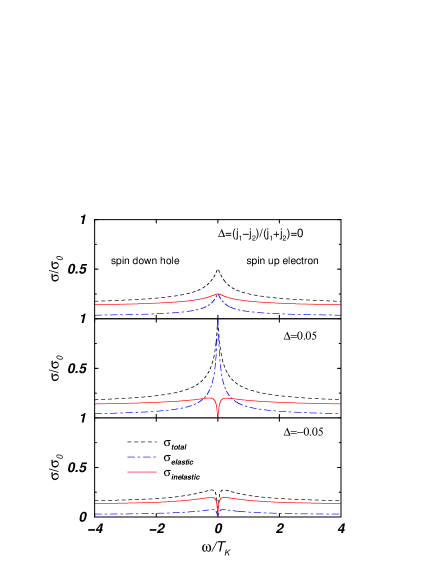
Figure 9: Energy dependence of elastic and inelastic scattering rates for the two-channel Kondo model in channel “1” in units of $\sigma_{0}=4\pi/p_{F}^{2}$, at $T=0$ and for different channel asymmetry, $\Delta\equiv(j_{1}-j_{2})/(j_{1}+j_{2})$. The curves correspond to $j_{1}+j_{2}=0.3$.

The inelastic scattering rates for the two-channel Kondo model are shown in Fig. 9 as a function of the energy of the incoming particle. In the channel-symmetric case inelastic processes are allowed even at $\omega=0$, which is a clear signature of the non-Fermi liquid behavior. The non-Fermi liquid nature is also reflected in the $\sim\sqrt{\omega}$ singularity of the scattering cross sections at $\omega=0$. Note that this cusp is much less pronounced in the inelastic scattering rate.

For $\Delta>0$ the total scattering rate approaches the unitary limit in channel “1” below the Fermi liquid scale $T^{*}$. For $\Delta<0$, on the other hand, the total scattering rate goes to 0 in channel “1” below the Fermi liquid scale $T^{*}$. In both cases, the inelastic scattering freezes out, and $\sigma_{\rm inel}(\omega)$ shows a dip below $T^{*}$, and it ultimately scales to 0 as

$$\sigma_{\rm inel}(\omega)\approx cst.\frac{\omega^{2}}{{T^{*}}^{2}}\;.$$

Note that the inelastic scattering cross-section is very similar for $\Delta>0$ and $\Delta<0$, while the total scattering contributions differs dramatically in these two cases.

VI Inelastic scattering in the Anderson model

As a final example, let us consider the Anderson model defined by the Hamiltonian,

$$H = \sum_{{\bf p}\sigma}\epsilon({\bf p})a^{\dagger}_{{\bf p}\sigma}a^{\phantom{\dagger}}_{{\bf p}\sigma}+\epsilon_{d}\sum_{\sigma}d^{\dagger}_{\sigma}d^{\phantom{\dagger}}_{\sigma}$$ (48)

$$+ Ud^{\dagger}_{\uparrow}d^{\phantom{\dagger}}_{\uparrow}d^{\dagger}_{\downarrow}d^{\phantom{\dagger}}_{\downarrow}+V\sum_{\sigma,{\bf p}}\left(c^{\dagger}_{{\bf p}\sigma}d^{\phantom{\dagger}}_{\sigma}+\textrm{h.c.}\right)\;,$$

where now $d_{\sigma}$ denotes the local d-level’s annihilation operator, $U$ is the on-site Coulomb repulsion, and the conduction band and the local electronic level are hybridized by $V$.

The $T$-matrix for the Anderson model can be related to the $d$-level’s Green’s function, as first discussed by Langreth. langreth The required relation can be trivially established the the path integral formalism presented in Section III. The final result of this derivation, which is to some extent discussed in Appendix A can be written as:

$${\rm Im}\{{\cal T}_{\sigma}(\omega)\} = \pi{V^{2}}\varrho_{d,\tau\sigma}(\omega)\;,$$

$$-\tau\ {\rm Re}\{{\cal T}_{\sigma}(\omega)\} = {V^{2}}\int d\omega^{\prime}\;\frac{\varrho_{d,\tau\sigma}(\omega)}{\omega-\omega^{\prime}}\;,$$ (49)

with $\varrho_{d,\sigma}(\omega)$ the spectral function of the $d$-Fermion’s spectral function, and $\tau={\rm sgn}\;\xi$.

The ground state of the Anderson model is of a Fermi liquid. Therefore, the Fermi liquid relations (45) can be used again to properly normalize the $T$-matrix. As we discussed in Ref. zar_inel, , the Fermi liquid relations also imply that at the Fermi energy the eigenvalue of the single particle $S$-matrix lies on the unit circle, and therefore the inelastic scattering rate vanishes.

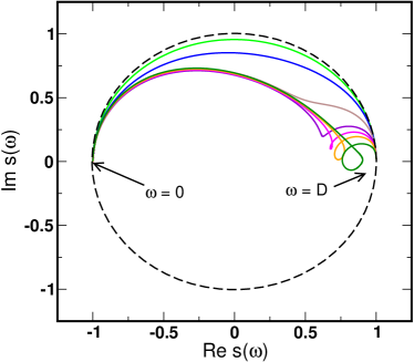
Figure 10: Flow of the eigenvalue of the $S$-matrix for the Anderson model for $\Delta=0.035$, $U=0.04$, $0.08$, $0.16$, $0.26$, $0.32$, $0.40$, $0.64$ and $\varepsilon_{d}=-U/2$.

The flow of the eigenvalue $s(\omega)$ is shown in Fig. 10. This flow diagram is very similar to that of the Kondo model at low energies, however, a new interesting feature appears at $\omega\sim U$, where $s(\omega)$ displays a hook. This hook corresponds to largely inelastic scattering processes, which are associated with the charge fluctuations of the d-level. It is adequate to mention here that the low energy flow is not completely identical to that shown in Fig.2 for the Kondo model. The reason is purely technical: For the Anderson model we were using the self-energy trick invented by Bulla and coworkersralf_selfenergy to obtain higher quality results, and computed the $\omega\sim T_{K}$ part of the $T$-matrix (especially its real part) much more accurately.

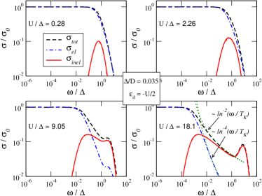
Figure 11: Elastic, inelastic and total scattering cross section for the symmetric Anderson model $\varepsilon_{d}=-U/2$, for various ratios of $U/\Delta$. For moderate values of $U/\Delta$ the effects of U are minor in the total and the elastic scattering rate, while for large values of $U/\Delta$ the various scattering rates for $\omega\ll U$ follow very nicely the behavior found for the Kondo model

These features also appear in the various scattering rates, shown in Fig. 11 for the symmetrical Anderson model with $\epsilon_{d}=-U/2$. There we show the inelastic scattering rate for various ratios of $U/\Delta$, $\Delta=\pi\varrho V^{2}$ being the width of the resonance. For moderate values of $U/\Delta$ the effects of U are minor in the total and the elastic scattering rate, however, rather surprisingly, one can see a clear maximum in the inelastic scattering rate at energies $\omega\sim U$ even in this case. Increasing $U/\Delta$, the Fermi liquid regime and the charging regime separate, and two distinct peaks appear, now even in the total and elastic scattering rates. For large values of $U/\Delta$ the various scattering rates follow very nicely the behavior found for the Kondo model at low energies, and for $T_{K}\ll\omega\ll U$ the elastic and inelastic contributions scale as $\sim 1/\ln^{4}(\omega/T_{K})$ and $\sim 1/\ln^{2}(\omega/T_{K})$, respectively. It is remarkable, that the Hubbard peak at $\omega\sim U$ is essentially entirely inelastic.

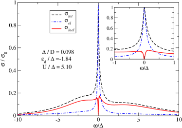
Figure 12: Elastic, inelastic and total scattering cross section for the asymmetric Anderson model. The low energy part of the curves is again very similar to the one obtained for the Kondo model.

Fig. 12 shows the same behavior on a linear scale for the asymmetrical Anderson model with moderate interaction strength. The low-energy part of the figure is again strikingly similar to the one obtained for the Kondo model. This is not very surprising, since the Kondo model is just the effective model of the Anderson model in the limit of large $U/\Delta$ and $\omega\ll U$, where charge fluctuations occur only virtually. It is remarkable that the quasi-linear behavior of $\sigma_{\rm inel}$ and the plateau are already present for these moderate values of $U/\Delta$.

VII Conclusion

In this paper, we discussed in detail the theory of inelastic scattering from quantum impurities at $T=0$ temperature, as formulated in Ref. zar_inel, , and applied this formalism to various cases. We computed numerically the flow of the $S$-matrix eigenvalues $s(\omega)$ for three prototypical examples of quantum impurity models, the Kondo model, the two-channel Kondo model, and the Anderson model. As we discussed, inelastic scattering appears, once $|s(\omega)|<1$, and the crucial difference between Fermi liquid models and non-Fermi liquid models is that for non-Fermi liquid models $|s(\omega)|<1$ even at the Fermi energy, $\omega\to 0$, while for Fermi liquids $|s(\omega=0)|=1$.

We also determined the inelastic scattering cross section, $\sigma_{\rm inel}(\omega)$, for all these models. For the Kondo model and the Anderson model in the Kondo regime, i.e., for large interaction values, the low-energy part of $\sigma_{\rm inel}(\omega)$ has features essentially identical to those of the Kondo model: Deep in the Fermi liquid regime one has $\sigma_{\rm inel}(\omega)\sim(\omega/T_{K})^{2}$, while for $0.05T_{K}<\omega<0.5T_{K}$ a quasi-linear regime appears, above which $\sigma_{\rm inel}$ exhibits a plateau with $\sigma_{\rm inel}(\omega)\approx cst$ over a wide frequency range. These features are quite robust, and survive even in the case of electron-hole symmetry breaking.

We also find that at large frequencies the scattering becomes asymptotically inelastic, and the inelastic scattering rate scales as

$$\frac{1}{\tau_{\rm inel}}\approx n_{\rm imp}\frac{\pi S(S+1)}{2\;\varrho\;\ln^{2}(\omega/T_{K})}\;.$$

while the elastic scattering rate falls off much more rapidly as

$$\frac{1}{\tau_{\rm el}}\approx n_{\rm imp}\frac{\pi^{3}S(S+1)}{8\;\varrho\;\ln^{4}(\omega/T_{K})}\;.$$

This result implies that –contrary to common wisdom– even spin-diagonal scattering is inelastic at high energies. Garst

In addition to these remarkable low-energy features, the Anderson Hamiltonian exhibits another, very interesting inelastic scattering peak at $\omega\sim U$ that corresponds to charge excitations. Rather surprisingly, this peak is present even in the weak coupling regime, where no Hubbard peak can be seen in the total scattering cross section. In the Kondo regime, on the other hand, this peak is essentially identical to the Hubbard peak that appears in the total scattering cross-section, and which corresponds to almost completely inelastic scattering.

In the two-channel Kondo model, the prototype of all non-Fermi liquid models, inelastic scattering remains finite even if $\omega\to 0$, and is exactly half of the total scattering rate. However, the tiniest channel symmetry breaking destroys this non-Fermi liquid state, and generates a new Fermi liquid scale, $T^{*}$, below which inelastic scattering freezes out, and the scattering becomes totally elastic.

The inelastic scattering rates computed here for the Kondo and Anderson models and their finite temperature versions computed in Ref. Rosch, are in quantitative agreement with recent experimental studies on magnetically doped mesoscopic wires excepting the limit of very small temperature, where a small residual inelastic scattering rate seems to be present. Saminadayar2005 ; Saminadayar2006 ; Birge2006 The origin of this small residual inelastic scattering rate is not clear yet, it might be due to some structural defects caused by the implantation process, or just some magnetic ions located at the interface of the wire. The agreement is even more surprising, since in reality, magnetic impurities are not of spin $S=1/2$ character, but have a rather complicated $d$-level structureZawareview . They thus usually have a large spin associated with them (typically $S=2$ or $S=5/2$ for for Fe, Cr, or Mn) subject to crystal fields, that does not couple through a simple exchange interaction to the conduction electrons. In reality scattering thus takes place in some $d$-electron channels. For $S=5/2$, e.g., the Fermi liquid state forms due to screening in five $d$-channels. Unfortunately, these realistic impurity models are out of reach for NRG computations.

In case of $d$-impurities, scattering cross-sections become also larger due to the many angular momentum channels that are open to scattering. Assuming spherical symmetry, e.g., the angle averaged total and elastic scattering cross sections become

$$\sigma_{\rm tot} = \frac{2\pi}{p_{F}^{2}}\sum_{L}\;{\rm Im}\{t_{L}(\omega)\}$$ (50)

$$\sigma_{\rm el} = \frac{\pi}{p_{F}^{2}}\sum_{L}|t_{L}(\omega)|^{2}\;,$$ (51)

i.e., the total, elastic and inelastic scattering cross-sections are about five times larger for $d$-wave scattering than for $s$-wave scattering considered in the usual Kondo problem. This must also be taken into account when computing the amplitude of the observed Kondo anomaly or that of the inelastic scattering rate. Finally, band structure effects may also play an important role in real materials, where the Fermi surface is not spherical, and the Fermi velocity depends on the direction of incidenceAchim2 .

Appendix A Field-Theoretic derivation of the T-matrix for the Anderson model

Here we derive the T-matrix for the Anderson model following the lines of Sec. III. We first introduce the generating functional for the Green’s functions

$$Z(\eta,\overline{\eta})=\int D[\overline{a}_{\sigma}a_{\sigma}]D[\overline{d}_{\sigma}d_{\sigma}]e^{-iS}e^{i\overline{\eta}a+i\eta\overline{a}},$$ (52)

where the source terms are defined as in Sec. III. The action $S=S_{e}+S_{d}+S_{hyb}+S_{int}$ consists of four distinct parts, with $S_{e}$ defined by Eq.(34) is identical to the one given in Sec.III and the remaining parts given by

$$S_{d} = -\sum_{\sigma}\int dtdt^{\prime}\overline{d}_{\sigma}(t)\left[G^{0}_{d}\right]_{\sigma}(t-t^{\prime})d_{\sigma}(t^{\prime})\;,$$

$$S_{hyb} = V\sum_{\sigma}\int dt\left(\overline{a}_{\sigma}(t,0)d_{\sigma}(t)+\textrm{c.c}\right)\;,$$

$$S_{int} = U\int dt\overline{d}_{\uparrow}(t)\overline{d}_{\downarrow}(t)d_{\downarrow}(t)d_{\uparrow}(t)\;,$$ (53)

respectively. Shifting the integration variables generates the terms

$$- \overline{\eta}\cdot a-\eta\cdot\overline{a}\to\sum_{{\bf{p}},\sigma}\int dtdt^{\prime}\overline{\eta}_{{\bf{p}},\sigma}G^{0}_{{\bf{p}}\sigma}(t-t^{\prime})\eta_{{\bf{p}},\sigma}-V\sum_{{\bf{p}},\sigma}\int dtdt^{\prime}G^{0}_{{\bf{p}}\sigma}(t-t^{\prime})\left(\overline{\eta}_{{\bf{p}},\sigma}(t^{\prime})d_{\sigma}(t)+\textrm{c.c.}\right)\;,$$

and which, after functional differentiation with respect to $\eta_{{\bf{p}},\sigma}$, give rise to the identity

$$G_{{\bf{p}}\sigma,{\bf{p^{\prime}}}\sigma^{\prime}}(t-t^{\prime})=\delta_{{\bf{p}},{\bf{p^{\prime}}}}\delta_{\sigma,\sigma^{\prime}}G^{0}_{{\bf{p}}\sigma}(t-t^{\prime})-iV^{2}\delta_{\sigma,\sigma^{\prime}}\int d\tilde{t}d\tilde{t}^{\prime}G^{0}_{{\bf{p}}\sigma}(t-\tilde{t})\langle d_{\sigma}(\tilde{t})\overline{d}_{\sigma^{\prime}}(\tilde{t}^{\prime})\rangle G^{0}_{{\bf{p^{\prime}}}\sigma^{\prime}}(\tilde{t}^{\prime}-t^{\prime}).$$

The Fourier transform of this equation yields Eq.(49).

References

- (1) F. Pierre and N. O. Birge, Phys. Rev. Lett. 89, 206804 (2002).
- (2) F. Schopfer, C. Bäuerle, W. Rabaud, and L. Saminadayar Phys. Rev. Lett. 90, 056801 (2003); For earlier measurements see C. Van Haesendonck, J. Vranken, and Y. Bruynseraede, Phys. Rev. Lett. 58, 1968 (1987).
- (3) F. Pierre, A. B. Gougam, A. Anthore, H. Pothier, D. Esteve, and N. O. Birge, Phys. Rev. B 68, 085413 (2003).
- (4) A. Benoit, D. Mailly, P. Perrier, and P. Nedellec, Superlattices Microstruct. 11, 313 (1992).
- (5) For a review see,e.g., B.L. Altshuler, in Les Houches Lecture Notes on Mesoscopic Quantum Physics (edited by A. Akkermans et al., Elsevier, 1995).
- (6) P. Mohanty, E. M. Q. Jariwala, and R. A. Webb, Phys. Rev. Lett. 78, 3366 (1997); P. Mohanty and R. A. Webb, Phys. Rev. B 55, 13452 (1997).
- (7) P. Mohanty and R. A. Webb, Phys. Rev. Lett. 91, 066604 (2003).
- (8) D. S. Golubev and A. D. Zaikin, Phys. Rev. Lett. 81, 1074 (1998).
- (9) I. L. Aleiner, B. L. Altshuler and M. E. Gershenson, Waves in Random Media 9, 201 (1999).
- (10) J. von Delft, cond-mat/0510563; J. von Delft, in Fundamental Problems of Mesoscopic Physics, edited by I.V. Lerner et al. (Kluver, London, 2004), p.115-138.
- (11) A. Zawadowski, Phys. Rev. Lett. 45, 211 (1980); K. Vladár and A. Zawadowski, Phys. Rev. B 28, 1546 (1983); 28, 1582 (1993); 28, 1596 (1983).
- (12) Y. Imry, H. Fukuyama and P. Schwab, Europhys. Lett. 47, 608 (1999).
- (13) G. Zaránd, L. Borda, J. von Delft and N. Andrei, Phys. Rev. Lett. 93, 107204 (2004).
- (14) H. Pothier, S. Guéron, N. O. Birge, D. Esteve, and M. H. Devoret, Phys. Rev. Lett. 79, 3490 (1997).
- (15) B. L. Altshuler, A. G. Aronov, and D. E. Khmelnitskii, J. Phys. C 15, 7367 (1982).
- (16) A. A. Abrikosov, Physics 2, 21 (1965). Phys. Rev. 138, A1112 (1965); H. Suhl, Phys. Rev 138, A515 (1965).
- (17) A. Kaminski and L. I. Glazman, Phys. Rev. Lett. 86, 2400 (2001).
- (18) G. Göppert, Y. M. Galperin, B. L. Altshuler, and H. Grabert, Phys. Rev. B 66, 195328 (2002).
- (19) J. Sólyom and A. Zawadowski, Z. Phys. 226, 116 (1969).
- (20) J. Kroha and A. Zawadowski, Phys. Rev. Lett. 88, 176803 (2002).
- (21) C. Bäuerle, F. Mallet, F. Schopfer, D. Mailly, G. Eska, and L. Saminadayar, Phys. Rev. Lett. 95, 266805 (2005).
- (22) F. Mallet, J. Ericsson, D. Mailly, S. Ünlübayir, D. Reuter, A. Melnikov, A. D. Wieck, T. Micklitz, A. Rosch, T. A. Costi, L. Saminadayar, and C. Bäuerle, Phys. Rev. Lett. 97, 226804 (2006).
- (23) G. M. Alzoubi and N. O. Birge, Phys. Rev. Lett. 97, 226803 (2006).
- (24) T. Micklitz, A. Altland, T. A. Costi, A. Rosch, Phys. Rev. Lett. 96, 226601 (2006).
- (25) T. Micklitz, T. A. Costi, A. Rosch, cond-mat/0610304.
- (26) J. J. Lin, private communication.
- (27) P. Mehta, N. Andrei, P. Coleman, L. Borda, G. Zaránd, Phys. Rev. B 72, 014430 (2005).
- (28) C. Itzykson and J. B. Zuber, Quantum Field Theory (McGraw-Hill, 1985).
- (29) K.G. Wilson, Rev. Mod. Phys. 47, 773 (1975); for a review see R. Bulla, T. A. Costi, T. Pruschke, cond-mat/0701105 (2007).
- (30) T. A. Costi, Phys. Rev. Lett. 85, 1504 (2000).
- (31) P. Mehta and N. Andrei, Phys. Rev. Lett. 96, 216802 (2006).
- (32) For a review see A.C Hewson, The Kondo Problem to Heavy Fermions, Cambridge University Press (1993).
- (33) D.L. Cox, A. Zawadowski, Adv. Phys. 47 599 (1998).
- (34) P. Nozières, J. Low Temp. Phys. 17, 31 (1974).
- (35) J. M. Maldacena and A. W. W. Ludwig, Nucl. Phys. B506, 565 (1997).
- (36) D. C. Langreth, Phys. Rev. 150, 516 (1966).
- (37) M. Le Bellac,Quantum and Statistical Field TheoryOxford Science Publications, 1991.
- (38) W. Koller, A. C. Hewson, D. Meyer, Phys. Rev. B 72, 045117 (2005).
- (39) M. Garst, P. Wölfle, L. Borda, J. von Delft, L. I. Glazman, Phys. Rev. B 72, 205125 (2005).
- (40) Y. Nagaoka Phys. Rev. 138, A1112 (1965); H. Suhl, Phys. Rev 138, A515 (1965).
- (41) L. Borda , G. Zaránd, W. Hofstetter, B. I. Halperin, and J. von Delft Phys. Rev. Lett. 90, 026602 (2003); For details, see W. Hofstetter and G. Zaránd, Phys. Rev. B 69, 235301 (2004).
- (42) In Ref. Nozieres Nozières considers stable quasiparticles rather than electrons, which do not decay at .
- (43) N.Andrei, C.Destri, Phys. Rev. Lett. 52, 364 (1984).
- (44) I. Affleck and A.W.W. Ludwig, Phys. Rev. B 48, 7297 (1993).
- (45) R. Bulla, A. C. Hewson, T. Pruschke, J. Phys.: Condens. Matter 10 8365 (1998).
- (46) For a review see, e.g., G. Grüner and A. Zawadowski, Rep. Prog. Phys. 37, 1497 (1974).
- (47) N. Andrei, K. Furuya and J. H. Lowenstein, Rev. Mod. Phys.55 331 (1983); A. M. Tsvelik and P. B. Wiegmann, Adv. Phys. 32, 453 (1983).