Metal clusters, quantum dots and trapped atoms – from single-particle models to correlation

Abstract

In this review, we discuss the electronic structure of finite quantal systems on the nanoscale. After a few general remarks on the many-particle physics of the harmonic oscillator – likely being the most studied example for the many-body systems of finite quantal systems, we turn to the electronic structure of metal clusters. We discuss Jahn-Teller deformations for the so-called ’ultimate’ jellium model which assumes a complete cancellation of the electronic charge with the ionic background. Within this model, we are also able to understand the stable electronic shell structure of tetrahedral (3D) or triangular (2D) cluster geometries, resembling closed shells of the harmonic confinement, but for Mg clusters being “doubly-magic” as the electronic shells occur at precisely twice the atom numbers in the close-packed tetrahedra. Taking a turn to the physics of quantum dot artifical atoms, we discuss the electronic shell structure of the quasi two-dimensional, harmonically confined electron gas. Between the clear shell closings, corresponding to the magic numbers in 2D, Hund’s rule acts, maximizing the quantum dot spin at mid-shell. After a brief excursion to multicomponent quantum dots and the formation of Wigner molecules, we turn to finite quantal systems in strong magnetic fields or, equivalently, electron droplets that are set highly rotating. Working within the lowest Landau level, we draw the analogy between magnetic fields and rotation, commenting on the formation of the so-called maximum density droplet (MDD) and its edge reconstruction beyond the integer quantum Hall regime. Formation and localization of vortices beyond the MDD, as well as electron localization at extreme angular momenta, are discussed in detail. Analogies to the bosonic case, and the systematic build-up of the vortex lattice of a rotating Bose-Einstein condensate at high angular momenta, are drawn. With our contribution we wish to emphasize the many analogies that exist between metallic clusters, semiconductor artificial atoms, and cold atoms in traps.

and

1 Introduction

One common feature of most small quantum-mechanical systems is the discreteness of the quantum states. In systems with high symmetry the single-particle energy levels are degenerate, which may lead to shell structure. This is known to happen in free atoms, but also in nuclei [1]. Spherical metal clusters [2], where the particles move in a spherically symmetric mean field, provide another example. In semiconductor quantum dots with circular symmetry, shell structure was observed by conductance spectroscopy by Tarucha et al. [3]. (For a review, see [4]). The ’universality’ of shell structure bridges these fields of physics. However, there are also fundamental differences: In atoms and in quantum dots, the fixed external potential dominates, leading to Hund’s rule with maximum spin at mid-shell to resolve the degeneracy of the spherical confinement. The valence electrons in metal clusters, or the neutrons and protons of a nucleus, however, move in a mean-field potential determined solely by the particle dynamics. To resolve degenaracies for non-closed shells, metal clusters and nuclei exhibit spontaneous shape deformation, while atoms and quantum dots do not. Consequently, the often used name ’artificial atom’ is well suited for semiconductor quantum dots, but would be misleading for free metal clusters.

Many properties of metal clusters can be calculated by using so-called ab initio electronic structure calculations and molecular dynamics. These computational results often are in very good agreement with experimental data – as, for example, in photoemission spectroscopy. They can pin-point the detailed ground-state geometries of particular cluster sizes [5]. However, many overall features can even be understood using simple models [2, 6]. This also holds for semiconductor quantum dots, where often, simple single-particle models have been very successful [4].

The purpose of this (brief, and by no means complete) review is to summarize the simple models, their advantages and limitations in describing overall properties of metal clusters and quantum dots, and to draw analogies between these finite quantal systems to the more recently emerging field of cold (bosonic or fermionic) atom gases in traps.

Let us begin by looking at the simple, but relevant many-particle physics of the harmonic oscillator. These results are then applied to understand the jellium model for metal clusters and electronic states in quantum dots. The universality of deformation is shortly described using simple models. We finally turn to a comparsion of quantum dots at strong magnetic fields, and weakly interacting bosonic systems that are set rotating.

2 Many-particle physics in harmonic oscillator

The harmonic oscillator confining a single-particle is solved in about all text books of quantum mechanics. However, adding more particles immediately makes it more challenging to describe the system theoretically, and new interesting phenomena appear. The many-body Hamiltonian is then written as

$$H=\sum_{i}\left(-\frac{\hbar^{2}}{2m}\nabla_{i}^{2}+\frac{1}{2}m\omega_{0}^{2}r_{i}^{2}\right)+\sum_{i\neq j}v(|{\bf r}_{i}-{\bf r}_{j}|),$$ (1)

where $\omega_{0}$ is the frequency of the confining harmonic oscillator and $v(r)$ the interparticle two-body interaction. The position vector $r_{i}$ and the Laplace operator $\nabla_{i}^{2}$ may be three-, two- or one-dimensional depending on the system in question. Sometimes we want to use the occupation number representation and write

$$H=\sum_{i,\sigma}\epsilon_{i}c_{i,\sigma}^{+}c_{i,\sigma}+\sum_{\{i,\sigma\}}v_{i_{1},i_{2},i_{3},i_{4}}c_{i_{1},\sigma_{1}}^{+}c_{i_{2},\sigma_{2}}^{+}c_{i_{4},\sigma_{4}}c_{i_{3},\sigma_{3}},$$ (2)

where $c^{+}$ and $c$ are the normal creation and annihilation operators (as here, for fermions), and $\epsilon_{i}$ is the single-particle energy of the form $\epsilon_{i}=\hbar\omega_{0}(n_{i}+d/2)$, $d$ being the dimension of the system. Most conveniently, one uses the single-particle states of the confining harmonic oscillator as a basis. It is important to note that even if the spin index appears in this formulation of the Hamiltonian (as a summation index), here we consider only spinless interactions, i.e. the Hamiltonian is, as obvious from Eq. (1), independent of the spin.

The perhaps most important feature of a harmonic confinement is, that the center-of-mass motion separates from the internal motion, regardless of the interaction between the particles. This can easily be shown for both classical and quantum systems [7]. As a consequence, the selection rule for the dipole oscillations only allows the center-of-mass excitation. In the case of simple metal clusters and quantum dots this is the plasmon resonance, with energy $\hbar\omega_{0}$, where $\omega_{0}$ is the frequency of the harmonic confinement [6]. In connection with two-dimensional quantum dots [8, 9, 10, 11, 12], the effect of the separation of the center-of-mass motion was earlier often referred to as “Kohn’s theorem” [13]. In the case of atomic nuclei, the related excitation is called the “giant resonance”, where the proton and neutron distributions oscillate with respect to each other [1].

Another important property of the harmonic confinement is the separation of the spatial coordinates from the center-of-mass motion (or single-particle motion). This means that the level structure in the most general case (with different oscillation frequencies $\omega_{i}$ along different directions) is simply

$$\epsilon_{n_{1},n_{2},n_{3}}=\hbar\omega_{1}(n_{1}+\frac{1}{2})+\hbar\omega_{2}(n_{2}+\frac{1}{2})+\hbar\omega_{3}(n_{3}+\frac{1}{2}).$$ (3)

For spherically symmetric potentials, labelling the energy levels by their radial and angular momentum indices, one obtains the harmonic energy shells given in Table 1. Including the spin degree of freedom with a factor of two, the “magic numbers” of the harmonic oscillator in three dimensions occur at particle numbers $2,8,20,40,70,...$, and at $2,6,12,20,30,42,...$ in two dimensions.

Table 1: Shell structure of three and two-dimensional (3D and 2D) harmonic oscillators. $g$ is the degeneracy of the shell and $N$ the cumulatice number of states without spin degeneracy.

		3D				2D
shell	levels	g	$N$	$2N$	g	$N$	$2N$
1	$1s$	1	1	2	1	1	2
2	$1p$	3	4	8	2	3	6
3	$2s1d$	6	10	20	3	6	12
4	$2p1f$	10	20	40	4	10	20
5	$3s2d1g$	15	35	70	5	15	30
6	$3p2f1h$	21	56	112	6	21	42

In a non-harmonic potential, the additional degeneracy of different radial states disappears, and other degeneracies occur. A famous example is the Wood-Saxon potential,

$$V_{\rm WS}(r)=-\frac{V_{0}}{1+e^{(R-r)/a}}~{},$$ (4)

frequently used in nuclear physics (where the spin-orbit interaction of the nucleons further splits the shells [1]). Single-particle states in this potential are filled following the sequence $1s,1p,1d,2s,2p,1f,$ etc. . The Woods-Saxon potential Eq. (4) is a good approximation for the mean-field potential in metal clusters [14], with energetically dominant magic numbers at 2, 8, 20, 40, 58, 92, etc. Note, however, that the first few magic numbers, as here $2,8$ and 20, are mainly determined by the angular momentum degeneracy and are nearly independent of the radial shape of the spherical potential.

In the 2D harmonic confinement the noninteracting electron states can be solved analytically also in the presence of a magnetic field [4], the resulting single-particle states being the so-called Fock-Darwin states [15, 16, 17]. Consequently, the harmonic confinement has been widely utilized when studying the quantum Hall effect in finite systems [18].

3 Jellium model of metal clusters

Many properties of simple metals, like alkalis, alkali earths and even aluminum can be explained as properties of the interacting, homogeneous electron gas. The role of the ions is then merely to keep the electron gas together at its equilibrium density. In the jellium model [20], inside the metal the charge of the ions is smoothened out and replaced by a homogeneous background charge with the same density as the electron gas. At the surface, the background charge goes abruptly to zero. The electron density is usually described by the density parameter $r_{s}$ defined as the radius of a sphere (in units of Bohr radius) containing one electron: $4\pi r_{s}^{3}/3=1/n_{0}$, with $n_{0}$ being the number density of the electrons. The density functional method in the local density approximation (LDA) is ideally suited for the jellium model which naturally has a smooth and slowly varying electron density.

This approach was first used to study metal surfaces [19], lattice defects [21] and impurities in metals [22]. The first application to metal clusters was made by Martins et al. [23], who studied the size variation of the ionization energy. Similar work had been successful for calculating the work function of planar surfaces of alkali metals [24].

In the density functional Kohn-Sham method the electrons more in an effective mean-field potential

$$V_{\rm eff}^{\sigma}({\bf r})=-e\phi({\bf r})+V_{\bf xc}^{\sigma}({\bf r}),$$ (5)

where $\phi$ is the total electrostatic potential of the background charge and electron density distribution, and $V_{\rm xc}$ is the exchange-correlation potential which depends locally on the electron density and spin polarization [25]. In the case of a spherical jellium cluster the effective potential resembles a finite potential well with rounded edge. It can be well approximated by the above mentioned Woods-Saxon potential (Eq. 4). The spherical jellium model suggests that, like in free atoms, the ionization potential is largest for the magic clusters, and at a minimum when only one electron occupies an open shell. The experimental results, however, show a much richer structure as a function of the cluster size, which in alkali metals is dominated by a marked odd-even staggering [2]. The reason behind are shape deformations, as described in the next section.

In the spherical jellium model for metal clusters, the the background charge is a homogeneously charged sphere of radius $R=\sqrt[3]{N}r_{s}$. The (external) potential caused by this sphere is

$$V_{\rm sphere}(r)=\left\{\begin{array}[]{ll}-\frac{Ne^{2}}{8\pi\epsilon_{0}R^{3}}\left(3R^{2}-r^{2}\right)&\textrm{if $r\leq R$}\\ -\frac{Ne^{2}}{4\pi\epsilon_{0}r}&\textrm{if $r>R$}~{}.\\ \end{array}\right.$$

Note that the potential inside the sphere is harmonic and can be written as

$$V_{\rm sp}(r)=\frac{1}{2}m\omega_{\rm sp}^{2}r^{2},$$ (6)

where

$$\omega_{\rm sphere}^{2}=\frac{e^{2}}{4\pi\epsilon_{0}r_{s}^{3}m}=\frac{n_{0}e^{2}}{3\epsilon_{0}m}=\frac{\omega_{p}^{2}}{3}$$ (7)

is the square of the plasmon frequency of a metallic sphere. Since the electrons only slightly spill out from the region of the harmonic potential, the plasmon is the dominating dipole absorption mechanism for spherical jellium clusters [6]. Ekardt [26] used the spherical jellium model in connection with the time-dependent density functional theory to study optical absorption. He found that the anharmonicity of the background potential caused fragmentation of the single plasmon peak to a distribution of close-lying absorption peaks. Similar work was subsequently done by several groups, using the RPA method [6, 27].

Koskinen et al. [28] used shell-model methods from nuclear physics to try to solve the electronic structure and photo-absorption of the jellium clusters beyond the mean-field approach. For up to eight electrons, they could diagonalize the many-electron Hamiltonian nearly exactly. Already for 20 electrons, however, the configuration interaction method showed a much too slow convergence as a function of the size of the basis set (in fact, it was shown that the error in the correlation energy was $\propto E_{\rm cut-off}^{-3/2}$). For eight electrons, their result agreed with those of the RPA calculations. For positively charged jellium spheres, the fragmentation of the plasmon peak disappears as the confinement of the electrons becomes harmonic [29, 28].

Historically, it is interesting to note that Martins et al. [23] corrected the pure jellium results by including ion pseudo-potentials via first-order perturbation theory, in a similar fashion than Lang and Kohn [20] had done for metal surfaces. While for planar surfaces the correction had only a minor effect (in alkali metals), it became dominating for large metal clusters, and completely diminished the effects of the electronic shell structure of the pure jellium sphere. A similarly large effect of the pseudopotential correction was observed for large voids in metals, shown to be due to the low-index surfaces present in spherical systems cut from an ideal lattice [31]. The notion of the possible importance of the lattice potential made the theoreticians cautious in making too strong predictions of the applicability of the jellium model to real metal clusters [32, 33], until the magic numbers of alkali metal clusters were observed [34].

The degeneracy of the open shell clusters should lead to Hund’s rules like in the case of free atoms. In the spherical jellium models the clusters with open shells should have a large total spin and magnetic moment [32]. This was predicted prior to the success of the jellium model by Geguzin [35], who studied highly symmetric cub-octahedral Na₁₃ clusters. For free clusters, however, deformation wins over Hund’s rule and removes both the degeneracy and magnetism [36].

We conclude that the simple spherical shell structure explains well the magic numbers in the experimental mass spectra of sodium clusters. It lies behind the so-called super shells [37, 38] observed in alkali metal clusters [39], as well as the importance of the collective plasmon resonance.

The simple jellium model also accounts for some properties of noble metals. Recently, it has been observed that even in gold clusters some features can be explained most easily with arguments based on the jellium model [40].

4 Deformed jellium

The similarity of small nuclei and simple metal clusters is not limited to magic numbers and to the existence of the plasmon-type giant resonance, but extends even to the internal deformation of the system. It is clear that the smallest clusters can be viewed as well-defined molecules with a geometry determined by the atomic configurations. Quantum chemistry can be used to characterize the ground state and spectroscopic properties of clusters with only a few atoms. For larger clusters ($N>10$) the early theories assumed spheres cut from a metal lattice [30], or faceted structures with shapes determined by the Wulff polyhedra [41]. In reality, however, the clusters exhibit geometries very different from these ideal structures. Many metals form icosahedral clusters [42, 43]. Jahn-Teller deformations are important even in quite large clusters, as manifested, for example, by the odd-even staggering of the ionization potential [2].

In the early cluster beam experiments, the temperature of the clusters was lowered only by evaporative cooling. The resulting cluster temperatures were so high that the clusters were most likely liquid [44]. The clusters showed the electronic shell structure as well as deformation, as determined by the splitting of the plasmon peak [45]. In fact, the super-shell structure could only been seen in liquid sodium clusters. Solid clusters formed icosahedral structures which governed the abundance and ionization potential spectra [46].

To model cluster deformations, Clemenger [47] was the first to apply the Nilsson model familiar from nuclear physics [1]. He was able to explain qualitative features of the abundance spectrum of sodium clusters, including the observed odd-even staggering. A more general model, based on the Strutinsky-model of nuclei [48], was developed by Reimann et al. [49], and applied to triaxial geometries by Yannouleas and Landmann [50] as well as Reimann et al. [51, 52]. It could explain nearly quantitatively the stabilities and deformation of small sodium clusters.

4.1 Ultimate jellium model

The simplest way to include deformation in the jellium model is to assume the uniform background charge density to be a spheroid, or an ellipsoid [53]. The model explains qualitatively the splitting of the plasmon peak and the size dependence of the ionization potential of alkali metal clusters. However, the optimal deformation shape determined by the electronic structure is not an ellipsoid, but a more generally shaped jellium background [54]. In the ultimate limit, the energy is minimized, when the background density equals the electron density – as suggested by Manninen already in 1986 [55]. In this so-called ’ultimate jellium model’ (UJM) [56], the density of the background is not fixed, but in a large cluster adjusts itself to correspond to $r_{2}\approx 4.2~{}a_{0}$, a value close to the equilibrium electron density in sodium. (Here, $a_{0}$ is the Bohr radius). The ground-state densities for clusters with $N=2$ to 22 electrons are shown as constant density surfaces in Fig. 1.

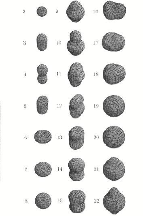
Figure 1: Constant-density surfaces of ’ultimate jellium’ clusters with up to 22 electrons. After Koskinen et al., see Ref. [56] for details and scales).

Clearly, the magic numbers at small $N$, here for 2, 8, and 20 electrons, correspond to spherical symmetry of the freely deformable ’ultimate jellium’ droplet. Off-shell, however, the shapes of the clusters exhibit breaking of axial and inversion symmetries. In general, the resulting ground-state geometries are far from ellipsoidal. Clusters which lack inversion symmetry, are very soft against odd-multipole deformations [56].

Remarkably, the results obtained from the UJM for deformations are very close to those of ab initio calculations for sodium [57], as shown in Fig. 2 and Fig. 3.

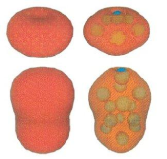
Figure 2: Comparison of shapes of UJM clusters (left) to those of DFT-LDA molecular-dynamics methods (right), for Na-6 (upper panel) and Na-14 (lower panel). In all cases the outer surface shown corresponds to the same particle density. Blue spheres represent the ions. From Ref. [58].

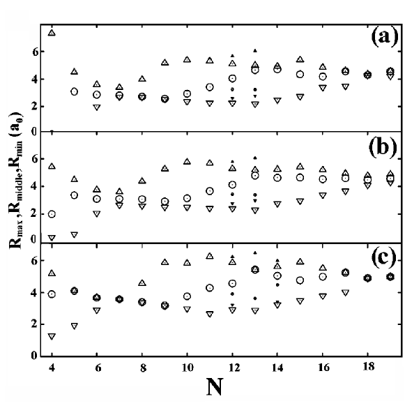
Figure 3: The three radii of the anionic sodium clusters along the principal axis, plotted vs the number of atoms in the cluster. Down-triangles, circles, and up-triangles correspond to $R_{\rm min}$ , $R_{\rm middle}$ , and $R_{\rm max}$, respectively. (a) Radii corresponding to the ground-state geometry of ab initio calculations, (b) thermally averaged radii from room-temperature simulations, (c) radii calculated within the UJM. From Ref. [57].

Koskinen et al. [59] applied the UJM to determine the shape deformations of small nuclei. Their method gave rather good agreement with experimental results, and surprisingly, nearly exactly the same geometries as for the electron-gas jellium. Häkkinen et al. [58] studied further the idea of this ’universal deformation’ and found that in the LDA, density functional theory predicts similar deformations for all small fermion clusters.

This shape universality can be easily understood in systems where the particles move in a mean field caused by the particles themselves. When the number of the particles is small, there is only a small number of single-particle states which determine the shape. For example, for four particles, only the $1s$ and, say, $1p_{x}$ states are filled. Consequently, the shape is prolate along the $x$-direction. This corresponds to the basis of the Nilsson model [1].

The robustness of the shape on the specific model was further studied by Manninen et al. [60], who showed that deformations of the UJM are in very good agreement with results of the ’ultimate’ tight-binding model: the Hückel model for clusters [61].

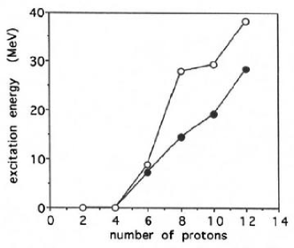
Figure 4: Left: Shape parameter $a_{20}$ for fermion clusters from 5 to 40 particles calculated with the UJM (black dots connected with solid line) compared to the experimental results for even-even nuclei (stars). Right: Excitation energies of linear isomers calculated with the UJM for nuclei (open circles) and compared to the experimental results (black dots). From Ref. [60].

For nuclei, the simple universal model only needs two parameters, the bulk modulus and the average binding energy per nucleon (the first term in the so-called mass formula [1]), to give good quantitative approximations to the deformation parameters and even excitation energies of shape isomers, as shown in Fig. 4.

4.2 Triangles and tetrahedra

The jellium model has also been aplied to quasi two-dimensional clusters, as for example in the early studies by Kohl et al. [62, 63]. A physical realization of two-dimensional clusters could be sodium clusters on an inert surface, or even two-dimensional electron-hole liquids in semiconductors. Reimann et al. [64] analyzed systematically the UJM ground-state shapes for quasi two-dimensional sodium clusters. Contours of the self-consistent ground-state densities of these two-dimensional fermion droplets are shown in Fig. 5, calculated for a 2D layer thickness of 3.9$a_{0}$.

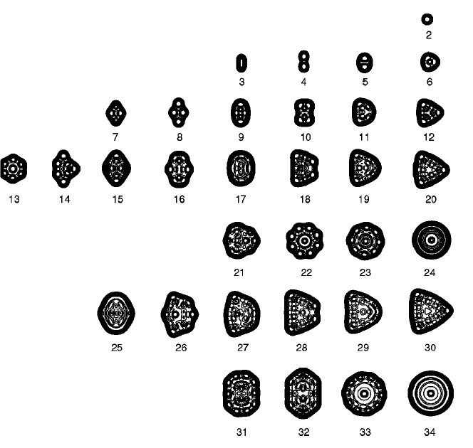
Figure 5: Contours of the self-consistent ground-state densities of two-dimensional UJM clusters for electron numbers $N\leq 2\leq 34$, calculated for a 2D layer thickness of 3.9$a_{0}$. From Ref. [64] (see this Ref. for details).

The shape systematics reveals that for electron numbers 6, 12, 20, and 30 the 2D clusters have triangular shape. Initially, this result appeared puzzling, as these shell closures correspond to those of the circular two-dimensional harmonic oscillator, and one should thus expect azimuthal symmetries of the ground-state densities. The explanation was, however, that in 2D, a triangular cavity has precisely these magic numbers [65], and only in the large-$N$ limit, the increased surface tension at the corners makes the oscillator shells more stable. In 2D, the shell closings are rather weak, with favorable energy minima (gaps at the fermi level) appearing mainly in the small-$N$ limit. Given the freedom of unrestricted shape deformations, a pronounced odd-even staggering appears in the ground-state energies, as seen in Fig. 6.

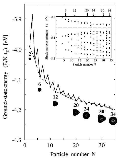
Figure 6: Ground-state energies per electron of two-dimensional clusters, as a function of cluster size $N$. (The kinetic energy contribution in $z$-direction, $t_{z}$, was subtracted). The inset shows the self-consistent single-particle Kohn-Sham energies for even particle numbers. From Ref. [64].

Incidentally, these shell fillings for the triangular geometries (without spin-degeneracy) equal precisely the number of atoms forming a close-packed triangle. In fact, the same holds in three dimensions: at small $N$, thetrahedral shell structure is prefered [66, 64], with magic numbers at $N=2,8,20,40,70$ and 112. These numbers correspond precisely to twice the numbers of atoms in a close-packed thetrahedral cluster geometry (see Fig. 7).

Figure 7: Left: Ground-state shape of the UJM for 112 electrons. Right: A possible structure of a Mg₃₅ cluster with 70 valence electrons. From Ref. [64].

One should expect that the compact tetrahedral geometry at an electronic magic number stabilizes theses clusters. However, first principles calculations have shown that this is not generally the case. Mg₁₀ has an overall tetrahedral shape, but is not a perfect tetrahedron [67]. Na₂₀ [68], and Mg₂₀ [67] are not tetrahedra, but Au₂₀ seems to be [69]. The experimental abundance spectrum of Mg shows a maximum at Mg₃₅ [70] – but so far, there is no evidence that its geometry is a tetrahedron like the one shown in Fig. 7. The above results suggests that trivalent metals on an oxide or graphite surface could favor triangular shapes.

In fact, advances in the experimental realization of surface-supported planar clusters have been recently reported by Chiu et al. [71]. They found magic numbers in quasi two-dimensional Ag clusters grown on Pb islands, and studied the transition from electronic to geometric shell structure.

We finally mention that high stability of tetrahedral shapes has also been discussed in nuclear physics [72, 73], predicting tetrahedral ground states for some exotic nuclei around ¹¹⁰Zr (see Schunck et al., [74]).

5 Semiconductor quantum dots

Generally speaking, a quantum dot is a system where a small number of electrons are confined in small volume in all three spatial directions. It can be, for example, a three-dimensional atomic cluster or a two-dimensional island of electrons formed by external gates in a semiconductor heterostructure [75, 4]. In this review, we shall only consider two-dimensional semiconductor quantum dots. Most often they are formed from AlGaAs-GaAs layered structures, where a low-density 2D conduction electron gas is formed in the AlGaAs layer. The quantum dot is formed by removing the electrons outside the dot region with external gates (lateral dot), or by etching out the material outside the dot region (vertical dot). In both cases, the resulting confining potential is, to a good approximation, harmonic. The underlying lattice of the semiconductor material can be taken into account by using an effective mass for the conduction electrons, and a static dielectric constant, reducing the Coulomb repulsion.

The resulting generic model for a semiconductor quantum dot is a 2D harmonic oscillator with interacting electrons. This in fact is like a 2D jellium model, with the simplification that now the harmonic confinement has infinite range and the center-of-mass motion separates out exactly (Kohn’s theorem [13]). This means that in the ideal case (in zero magnetic field) there is only one dipole absorption peak, as seen in experiments [76].

Conductance spectroscopy can be used on one single dot. The dot is weakly connected to leads and the current is measured as a function of the gate voltage which determines the chemical potential and thus the number of electrons in the dot [4]. When the electron number in the dot is large, the energy of an additional electron can be estimated from the capacitance $C$ of the dot, as $\Delta E=e^{2}/C$. The resulting conductance then shows equidistant peaks as a function of the gate voltage.

When the number of electrons is small, the individual single electron levels in the dot become important and their shell structure can be seen in the conductance spectrum. Tarucha et al. [3] were the first to successfully determine the shell structure of circular quantum dots. Their result is shown in the lower panel of Fig. 8, where the second derivative of the total energy of the dot is plotted as a function of the number of electrons, $N$. For comparison, the corresponding result of the LSDA calculation for electrons in a harmonic oscillator is included, too.

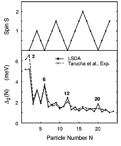
Figure 8: Second derivative of the total energy of electrons in a quantum dot as a function of the number of electrons. The magic numbers are shown. The experimental result is from Tarucha et al. [3]. The upper panel shows the calculated total spin.

The density functional Kohn-Sham method for semiconductor quantum dots usually assumes that $i$) the system is two-dimensional, $ii)$ only the conduction electrons are considered, with an effective mass $m^{*}$ and their Coulomb interaction screened by the static dielectric function $\epsilon$ of the material in question, and $iii)$ they move in a harmonic confinement $m\omega_{0}^{2}r^{2}$. A local approximation is used for the spin-dependent exchange-correlation energy, derived from the functionals for the 2D electron gas [77]. For details see Refs. [4].

Shell structure with main shell fillings (magic numbers) at $N=2,6,12,20$ appears very clearly in the addition energy differences $\Delta_{2}(N)$. (See Fig. 8). Furthermore, like in free atoms, due to Hund’s rule at mid-shell the total spin is maximal. This means that (just like for the spherical jellium model discussed above), any half-filled shell shows as a weak ’magic’ number, with increased stability. This is clearly seen in Fig. 8 where the second derivative of the total energy shows maxima at $N=4$ and $N=9$ in addition to the clear peaks at the filled shells, $N=2,6,$ and $12$. Figure 8 also shows the calculated total spin as a function of the number of electrons in the dot. The self-consistent data appear to agree very nicely with the experimental data. However, we notice that this agreement becomes worse with increasing $N$, showing very clear deviations between theory and experiment after the third shell, i.e. around $N=20$. Another series of experimental data, was later published by the same group in 2001. In Ref. [78], addition energies for 14 different quantum dot structures, all similar to the device used in the earlier work by Tarucha et al. [3], were analyzed. Strong variations in the spectra were reported, very clearly differing from device to device and seemingly indicating that each of these vertical quantum dots indeed has its own properties: a comparison to the theoreticalle expected shell structures needs to be taken with care. Progress with vertical quantum dots was achieved more recently, where few-electron phenomena could be studied by tunneling spectroscopy through quantum dots in nanowires [79, 80].

The self-consistent electronic structure calculations for quantum dots for some electron numbers showed internal symmetry-breaking of the spin-density [81], leading to a static “spin-density wave” (SDW). Figure 9 shows, as an example, the intriguing ground-state spin polarization for a quantum dot with six electrons. For not too small densities of the electron gas, i.e. $r_{s}\leq 6a_{0}^{*}$, this quantum dot still has a closed-shell configuration, with $S=S_{z}=0$. This result is obtained from SDFT. The total density obtained by the SDFT method is circularly symmetric, with zero net polarization ($S=0$). However, the spin polarization (which equals the difference between the spin densities $n^{\uparrow}-n^{\downarrow}$ normalized by the total density, $n^{\uparrow}+n^{\downarrow}$), in standard SDFT breaks the azimuthal symmetry of the confinement, showing a regular spin structure. Fig. 9 shows this very clearly for the example of a six-electron quantum dot at $r_{s}=4a_{0}$. Both spin-up and spin-down densities exhibit three clear bumps, which are twisted against each other by an angle of $\pi/3$. This resembles very much an antiferromagnet-like structure, with alternating up- and down spins, on a ring. Such states were obtained both with the Tanatar-Ceperley [77] as well as the more recent Attaccalite–Moroni–Gori-Giorgi–Bachelet (AMGB)  [82] functionals for exchange-correlation. As the AMGB functional depends explicitly on the spin polarization, there is left no doubt that the SDW states are not simply an artefact of the ad-hoc approximation to the correlation energy, which is usually interpolated following the polarization-dependance of the exchange energy [81].

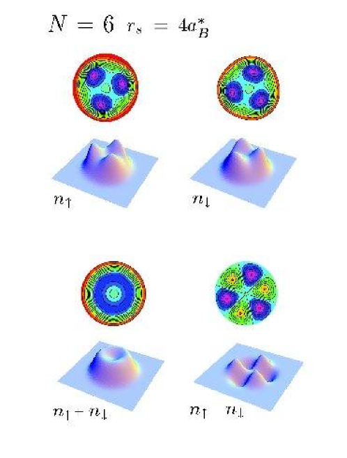
Figure 9: DFT spin densities $n^{\uparrow}$ and $n^{\downarrow}$ (upper panel) and total density ($n^{\uparrow}+n^{\downarrow}$) as well as (un-normalized) spin polarization ($n^{\uparrow}+n^{\downarrow}$) (lower panel) for a six-electron quantum dot at $r_{s}=4a_{0}^{*}$, shown as 3D plots and their contours. From Ref. [83].

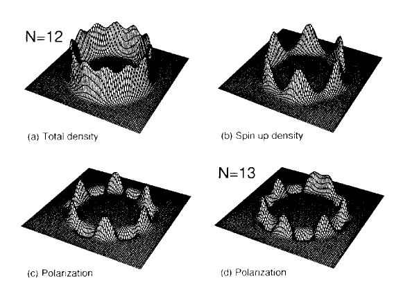
Figure 10: Quantum rings with $N=12$ and $N=13$ electrons, showing antiferromagnetic spin ordering along the ring. The maximum electron density in the 12-electron ring is at $n_{max}=0.157{a_{0}^{*}}^{-2}$. From Ref. [84].

In quasi-one-dimensional quantum rings (see section 7.2), these SDW states become more distinctive, as shown in Fig. 10.

The existence of the non-spherical spin-densities in quantum dots was disputed in the literature, since the spherical symmetry of the Hamiltonian dictates spherical symmetry [85, 86]. However, as well known from nuclear physics, a meal field theory (like KS-LSDA) can lead to internal symmetry breaking. In some cases [83] it reveals the internal structure which, in fact, can be very difficult to extract from the exact wave function. We will repeatedly meet this problem, for example when studying vortices and localization in rotating quantum systems, see Sections 6 and 6.4 below. (For further reading on the internal symmetry breaking, we refer to the recent review articles [4, 87, 88]).

The full quantum-mechanical problem of a few electrons in a 2D harmonic oscillator can be solved using the so-called configuration interaction (CI) technique, numerically diagonalizing a large Hamiltonian matrix. This method is often called “exact diagonalization”, although there is always an approximation due to the necessary restrictions in the basis set or the number of configurations included. Nevertheless, up to say 6 or even 10 particles (depending on the confinement strength) the results can be viewed as practically exact.

In general, the results of the exact diagonalization agree well with those obtained within the LSDA. The same spins dictated by the Hund’s rule are obtained and the total energies agree with good accuracy. Also, the electron-density and spin-density profiles are in excellent agreement. However, the exact diagonalization can reveal the existence of the internal symmetry breaking only via the pair correlation

$$g_{\sigma\sigma^{\prime}}({\bf r},{\bf r}^{\prime})=\langle\Psi|\hat{n}_{\sigma}({\bf r})\hat{n}_{\sigma^{\prime}}({\bf r}^{\prime})|\Psi\rangle$$ (8)

where $\Psi$ is the many-particle quantum state and $\hat{n}_{\sigma}$ the spin-density operator. This pair correlation function is also called as “conditional probability”, since it gives the probability of finding an electron with spin $\sigma^{\prime}$ at ${\rm r}^{\prime}$ when an electron with spin $\sigma$ is located at ${\bf r}$.

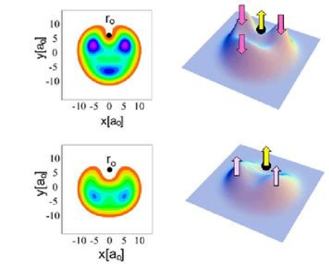
Figure 11: Pair correlations for a quantum dot with $N=6$ electrons, here at $r_{s}=3.8a_{0}^{*}$, obatined with the CI method. The top panel shows the (up,down)-correlations, the bottom panel the (up-up) correlations. The black dot marks the reference point, with given spin. From Ref. [83].

As an example, we show in Fig. 11 the pair correlations for the above discussed six-electron quantum dot, here at $r_{s}=3.8a_{0}^{*}$. The top panel shows the (up,down)-correlations, the bottom panel the (up-up) correlations. Clearly, the internal structure of the exact ground state resembles the SDFT result described above: The probability maxima appear on a ring, with six alternating maxima of the up- and down correlations.

For a more detailed discussion, we refer to the recent work by Borgh et al. [83] on broken-spin-symmetry in SDFT ground states and the reliability of SDFT. Here we only note that SDFT and CI results generally agree very well in the case of singlet states, as it was examplified above by the six-electron quantum dot. If the true ground state is a spin-multiplett, however, SDFT introduces an artificial splitting of multiplet states which may be misleading, and even become a real pitfall when determining ground state energies and symmetries where CI or other exact results to compare with, are not at hand.

5.1 Wigner molecules

The exact diagonalization method has also been used to study electron localization in low-density quantum dots. At extremely low densities, the homogeneous electron gas forms a Wigner crystal [89] also in the bulk. This happens in 3D, 2D and 1D, although in 1D the true long range order is fading with distance.

In three dimensions, the critical value at which crystallization occurs was determined to be $r_{s}=100a_{0}$ by Ceperley and Alder [90]. In two dimensions, the transition occurs at smaller $r_{s}$ values, according to Tanatar and Ceperley [77] at $r_{s}>37{a_{0}}^{*}$. Breaking of translational invariance in 2D lowers this value to $r_{s}\approx 7.5{a_{0}}^{*}$. Thus, in finite systems, localization may happen at even smaller values, as discussed, for example, by Creffield et al. [91], Egger et al. [92], or Yannouleas and Landmann [93].

For finite number of electrons in a quantum dot, the localized state is often called a “Wigner molecule” [92]. The local density approximation can not produce properly the localized states due to the lack of exact cancellation of the direct and exchange Coulomb interactions. The most direct notion of electron localization can be found by using the unrestricted Hartree-Fock approximation. The (complicated) mean-field character of the approach can lead to broken-symmetry solutions, showing the electron localization directly in the electron density [94, 93]. This method also indicates a clear “phase transition” point ($N$-dependent $r_{s}$) where the crystallization occurs. However, going beyond Hartree-Fock to the exact diagonalization results makes the situation more complicated: There is no clear phase transition in these finite systems, but the localization gradually becomes stronger when $r_{s}$ increases [95].

The most studied system in this context is the two-electron quantum dot, the so-called “quantum dot helium” [96], which is in some cases exactly solvable [97, 98, 99, 100, 101]. Zhub et al. [101] have shown that at low densities (weak confinement, small $\omega_{0}$) the many-particle excitation spectrum can be described with the rotation-vibration spectrum of two localized electrons. We will return to this method in the case of rotating systems in the next section.

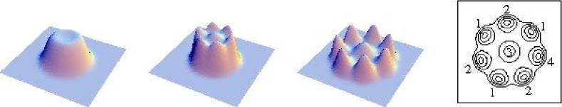
Figure 12: Electron density of a four-component quantum dot for three different strengths of the confinement frequency, corresponding to different values of the electron density parameter at the center of the dot: $r_{s}=2\ a_{0}$ (left), $6\ a_{o}$ (center), and $14\ a_{0}$ (right). The localization in the multicomponent LDA is made possible by the fact that the neighboring localized electrons belong to different components as indicated by the numbers in the contour plot.

As mentioned earlier, the LDA does not support electron localization due to the incomplete cancellation of the direct and exchange Coulomb interaction. The introduction of spin-dependence (LSDA) increases slightly the tendency of localization. If more internal degrees of freedom are included, as it could be done in the case of multi-valley semiconductors, the localization of electrons is expected to happen also in the local approximation. This possibility was studied by Kärkkäinen et al. [102]. Figure 12 shows the localization of 8 electrons in a multicomponent electron system when the confinement becomes weaker.

6 Rotating systems in 2D harmonic oscillator

A semiconductor quantum dot in the presence of a perpendicular magnetic field is a finite-size realization of the quantum Hall liquid (QHL), which has been an exciting system of study for both experimentalists and theorists. In fact, when Laughlin [18] suggested his celebrated wave function for the fractional quantum Hall state, he used exact diagonalization calculations for a finite quantum dot to test his ingenious Ansatz. Since then, it has been one of the systems used to mimic also the infinite systems in many-particle physics of QHL.

The conductance measurements through a quantum dot show that as a function of the magnetic field $B$, the conductance has rather complicated oscillations at small $B$-values [103]. These are caused by successive changes in the quantum states of the electrons, characterized by changes in the angular momentum and spin quantum numbers. However, at a certain field range the oscillations disappear and it is believed that the electrons form an integer QHL (with filling factor one). At this state the electron system is fully polarized.

The density functional theory has been extended to treat 2D electrons in the presence of magnetic fields [106]. In the so-called current-density functional method the exchange-correlation energy of the electrons depends, in addition to the electron density and polarization, also on the local current density of the electrons. Although the method can be disputed in being not uniquely defined in all cases and its functionals are not well established [104, 105], it has been useful in understanding the general ’phase diagram’ of the conductance, and has been successful to suggest new kinds of symmetry-broken ground states, with localized edge states [84, 107] and vortices [108] (see below) as prominent examples.

The perpendicular magnetic field in the 2D harmonic confinement has two effects: It interacts directly with the magnetic moments of the electrons causing a Zeeman term $g\mu_{B}S_{Z}B$, and changes the single electron kinetic energy from $p^{2}/2m$ to $({\bf p}-e{\bf A})^{2}/2m$. Using the symmetric gauge for the vector potential, ${\bf A}=(1/2)B(-y,x,0)$, and the definition of the cyclotron frequency $\omega_{c}=eB/m$ the single-particle Hamiltonian becomes

$$h=\frac{\hbar^{2}}{2m}\nabla^{2}+\frac{1}{2}m\left(\omega_{0}^{2}+\frac{1}{4}\omega_{c}^{2}\right)r^{2}+\frac{1}{2}\omega_{c}\hat{l},$$ (9)

where $\hat{l}$ is the $z$-component of the orbital angular momentum operator. Note that in 2D systems this is the only component, and thus, the same as the total angular momentum. We denote the single-particle angular momentum by $m$ and the many-particle angular momentum by $L$. Clearly, the single-particle problem is exactly solvable, as discussed already by Fock [15], Darwin [16], and Landau [17]. The single-particle energies can be written as

$$\epsilon_{nm}=\hbar\omega_{h}(2n+|m|+1)+\frac{1}{2}\hbar\omega_{c}l,$$ (10)

where $\omega_{h}=\sqrt{\omega_{0}^{2}+\omega_{c}^{2}/4}$ and the radial quantum number is $n=0,\quad 1,\quad,\cdots$ with the angular momentum $m$ being an integer. Figure 13 shows the single-particle states as a function of the cyclotron frequency (magnetic field). Only the levels with $|l|\leq 7$ are shown to illustrate clearly the separation of the levels to different Landau bands at large values of the magnetic field (large $\omega_{c}$). The lowest of these consists of states with $n=0$ and $m=0,\quad-1,\quad-2,\cdots$ in increasing order of energy.

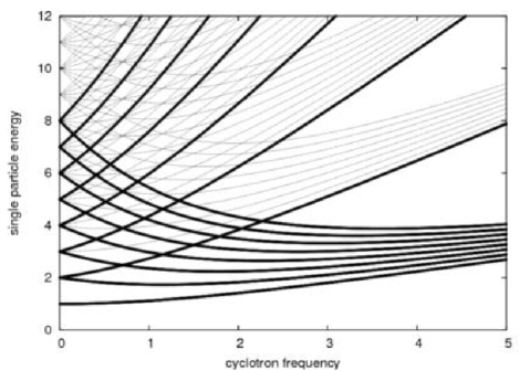
Figure 13: Single electron states in 2D harmonic oscillator in a perpendicular magnetic field. The levels are plotted as a function of the cyclotron frequency $\omega_{c}$. The levels with $n=0$ in Eq. (10) are shown as thick lines.

Normally, the Landé factor $g$ in the Zeeman energy is nonzero. Consequently, in a strong magnetic field the electron system will polarize. In this case, the non-interacting electrons fill the $N$ lowest energy states of the lowest Landau level (LLL). The single-particle states of the LLL are simply

$$\psi_{m}(r,\phi)=C_{m}r^{l}e^{-r^{2}/2\ell_{h}^{2}}e^{il\phi},$$ (11)

where $C_{m}$ is the normalization constant and $\ell_{h}=\sqrt{\hbar/m\omega_{h}}$ is the effective oscillator length. In the theory of QHL it is customary to describe the electron coordinates by a complex number $z=x+iy$, where $x=r\cos\phi$ and $y=r\sin\phi$. The ground state of polarized noninteracting electrons is a Slater determinant formed from the $N$ lowest single-particle states. Conveniently, it can be written (in the complex plane) as

$$\Psi_{MDD}(z_{1},z_{2},\cdots,z_{N})=\prod_{i<j}^{N}(z_{i}-z_{j})e^{-\sum|z_{k}|^{2}/2\ell_{h}^{2}},$$ (12)

where the normalization is omitted. This state is called the maximum density droplet (MDD) and is the finite-size analog of an infinite integer QHL. Note that the state is antisymmetric and has the total angular momentum $L_{MDD}=N(N-1)/2$.

The electron density of the MDD is constant inside the dot, as illustrated in Fig. 14, (note that the density of a single Slater determinant is simply $n(r)=\sum|\psi_{m}|^{2}$). In the case of non-interacting, polarized electrons the increase of the magnetic field does not change the structure of the system, but the MDD becomes smaller and smaller since $\ell_{h}$ decreases when $B$ (or $\omega_{c}$) increases. Before we turn to the much more interesting case of interacting electrons, let us note a few facts about the excited states of non-interacting fermions in the LLL.

The only way to excite electrons (for a fixed $B$ or $\omega_{c}$) in the LLL is to increase the single-particle angular momenta $m$ such that the total angular momentum increases by $\Delta L$. This gives an excitation energy of $\Delta E=\hbar\omega_{h}L$. However, the degeneracy of the state is in general large, since there are many ways to distribute the single-particle states in the LLL so that the total angular momentum is $L_{\rm MDD}+\Delta L$. The wave function can be written in the complex coordinates as

$$\Psi_{\delta L}=P(z_{1},z_{2},\cdots,z_{N})\prod_{i<j}^{N}(z_{i}-z_{j})e^{-\sum|z_{k}|^{2}/2\ell_{h}^{2}},$$ (13)

where $P$ is any homogeneous symmetric polynomial of order $\Delta L$. The proper antisymmetry is provided by the determinant $\prod(z_{i}-z_{j})$.

6.1 Interacting electrons in the LLL

The electron-electrons interactions can be included at different levels of approximations. The current-density functional theory in the LSDA takes into account the interactions on a mean-field level and allows to include the magnetic field as described above. Using the material parameters ($m^{*}$ and $\epsilon$) of GaAs, Reimann et al. [84] showed, in agreement with the experiments, that for each electron number there exists a region where the ground state is the maximum density droplet. This droplet slightly shrinks with increasing magnetic field. The “phase diagram” shown in Fig. 14 demonstrates how this region of MDD ground states becomes narrower when the number of electrons in the dot increases. (Here, the average electron density in the dot was chosen to be approximately constant, setting the confinement strength to $\hbar\omega=4.192N^{-1/4}$meV, which corresponds to a typical value for GaAs).

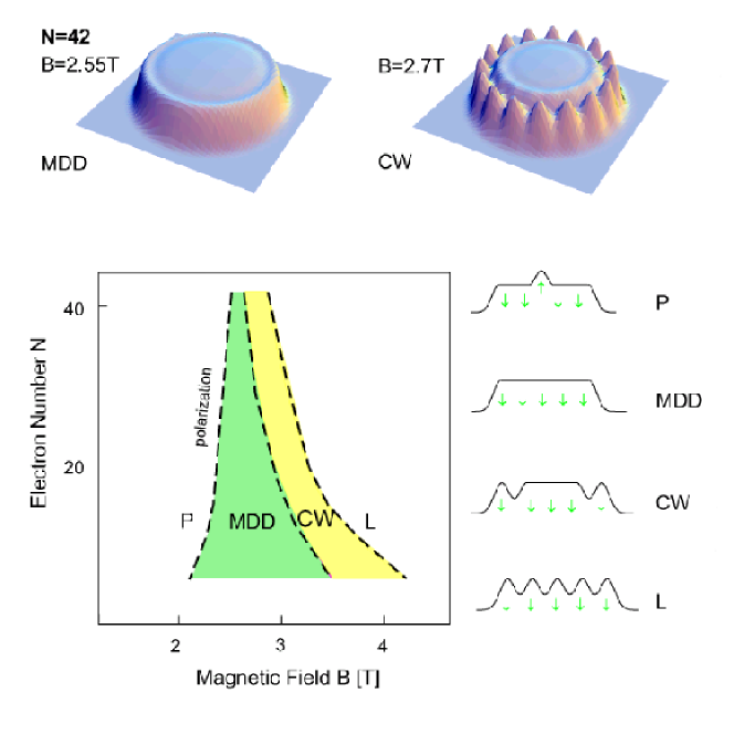
Figure 14: “Phase diagram” for electrons in a harmonic confinement in the presence of a magnetic field: P denotes the region of where the polarization happens, MDD is the maximum density droplet, CW is the region of the edge reconstruction, and L denotes the high-field region where electron localization sets in. Schematic densities and spin configurations of the different regions are shown at the right. The two figures on top show calculated electron densities for 42 electrons in the region of the MDD (left) and CW (right). The confinement strength was set to $\hbar\omega=4.192N^{-1/4}$meV, corresponding to typical GaAs values.

When the magnetic field becomes too large, the MDD breaks down. At large electron numbers, this begins from the surface of the droplet. A ring of electrons separates from the inner, still compact, droplet. The results current-density functional calculations suggest that in this split-off ring, the electrons are localized [84], as shown in Fig. 14. Again, this broken internal symmetry was disputed in the literature. However, calculations based on other many-particle methods have shown similar localization tendency of this so-called Chamon-Wen edge in the correlation functions [109, 110].

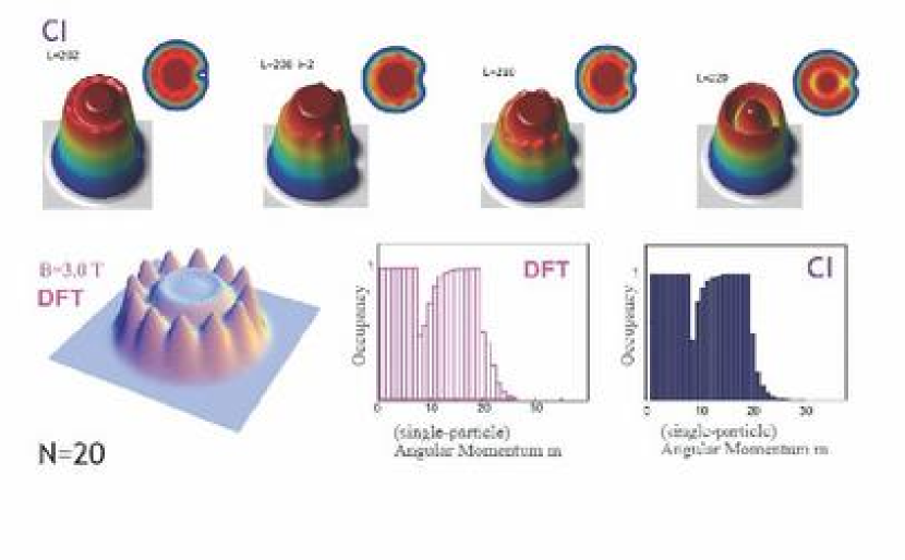
Figure 15: Comparison of CI correlation functions (upper panel) and mean-field densities, for a 20-electron quantum dot at high rotation, or equivalently, strong magnetic fields. The CI results were obtained for rotation in the Lowest Landau Level (LLL) only, for fixed angular momentum as specified. The mean-field result (lower panel, left) was calculated in CSDFT, at an effective magnetic field of $B=3.0T$ ($r_{s}=2{a_{0}}^{*}$). The two plots at the right-hand side of the lower panel compare the occupancies of the single-particle levels in the LLL, characterized by their single-particle angular momentum $m$.

Fig. 15 compares the correlation functions obtained from the CI calculations, to the corresponding result in mean-field current spin density functional theory (CSDFT). As an example, we here chose the 20-electron quantum dot at high rotation, or equivalently, strong magnetic fields. The broken-symmetry along the so-called Chamon-Wen edge is reproduced in the CI correlations. The occupancies of the single-particle levels in the LLL, characterized by their single-particle angular momentum $m$, agree remarkably well, demonstrating the success of CSDFT in describing the correlated electronic structure at strong magnetic fields.

6.2 Rotation versus magnetic field

A magnetic field applied to the 2D harmonic oscillator leads to the simple Hamiltonian Eq. (9). For a fixed angular momentum $l$ the last term of the Hamiltonian is a constant and the solutions are the harmonic oscillator energies and wave functions for the effective confinement $\omega_{h}=\sqrt{\omega_{0}+\omega_{c}/4}$. This is an important notion: we can equivalently study the rotational spectrum of the harmonic oscillator. For simplicity, we will now neglect the Zeeman effect, i.e. the direct interaction between the electron spins and the magnetic field, $g\mu_{B}S_{z}B$. (In fact, in semiconductors the effective Landé factor $g$ can be reduced to zero).

Similarly, for the many-particle system, even when the interactions are included, the effect of the magnetic field for a fixed $L$ is to increase the strength of the confinement. Clearly, the Hamiltonian can be written as

$$H=\sum_{i}\left(-\frac{\hbar^{2}}{2m}\nabla_{i}^{2}+\frac{1}{2}m\omega_{h}^{2}r_{i}^{2}\right)+\sum_{i\neq j}v(|{\bf r}_{i}-{\bf r}_{j}|)+\frac{1}{2}\omega_{c}\hat{L},$$ (14)

where now $\hat{L}$ is the total angular momentum. Again, if the total angular momentum is fixed, the last term reduces to a constant: in the case of a 2D harmonic confinement, the effect of the magnetic field is only to put the system in rotation, and to increase the strength of the confinement. In Fig. 16 the results of exact diagonalization for six electrons are shown for three different strengths of the field. Clearly, the relative structure of the spectra is very similar, and the effect of the field is only to tilt the spectrum towards higher angular momenta and to determine the energy scale via $\omega_{h}$. The rotational spectrum alone reveals all the effects the magnetic field can have (apart from the simple Zeeman term), making the direct comparison to other rotating systems (like for example, cold, atomic quantum gases) meaningful.

Figure 16: Many-particle energy spectrum as a function of the total angular momentum for three different values of the magnetic field (given in atomic units). From Ref. [111].

6.3 Localization of particles at high angular momenta

We will now study the interacting system in a rotational state with a very high angular momentum. First, let us consider fermions. For small particle numbers the exact diagonalization technique can be used with the harmonic oscillator states as the single-particle basis. When the angular momentum is large all the low energy states are in the lowest Landau level (LLL) as shown in Fig. 13, and the basis set can thus be restricted to include only the LLL. With this restriction the matrix size will be finite (for a fixed $L$) and for a small particle number no other approximations are needed.

Using the formalism of second quantization, the Hamiltonian for the polarized electrons (we drop the spin index) is

$$H=\sum_{l}\hbar\omega_{0}lc_{l}^{+}c_{l}+\sum_{\{i\}}v_{i_{1},i_{2},i_{3},i_{4}}c_{i_{1}}^{+}c_{i_{2}}^{+}c_{i_{3}}c_{i_{4}}.$$ (15)

For a fixed angular momentum $L$ the diagonal term of the Hamiltonian gives the energy $\hbar\omega_{0}L$ for all configurations, thus, just adding a constant. The diagonalization of the Hamiltonian is thus reduced to the non-diagonal interaction term. The effect of the confinement frequency $\omega_{0}$ (or $\omega_{h}$) is to provide the single-particle basis and to determine the energy scale through the interaction matrix elements $v_{i_{1},i_{2},i_{3},i_{4}}$. The many-particle states are completely independent of the confinement strength, when only the LLL is included in the basis. When studying the rotational energy spectrum, it is thus customary to plot the interaction energy, instead of the total energy. When the angular momentum of the system increases, the systems expands and the interparticle interactions decrease. The interaction energy then decreases with increasing angular momentum, as seen in the figures below.

Figure 17: Many-particle energy spectrum (the interaction energy) for 4 electrons in a harmonic confinement as a function of the angular momentum. The lowest energy states are connected with a line to illustrateal the period of four.

Figure 17 shows the energy spectrum calculated for four electrons as a function of the total angular momentum. Two features are distinct. First, each appearing new energy is repeated for all higher angular momentum values. This is due to the center-of-mass excitations. As discussed in Section 2, the center-of-mass motion separates from the internal motion, and its excitation energy is $\hbar\omega_{0}n$. In the LLL, each center-of-mass excitation increases the angular momentum by $\Delta L=1$, but since this does not change the interaction energy, it remains constant.

The second important feature of Fig. 17 is the periodic oscillation of the lowest energy state as a function of the angular momentum. These ’yrast’ states, i.e. the states with highest possible angular momentum at a fixed energy, are connected with a continuous line in the Figure. (Actually, the name ’yrast’ comes from Swedish language for “the most dizzy”, and originates from nuclear physics [112, 1]. The periodic oscillation, which becomes more distinct when the angular momentum increases, is a caused by localization of the electrons [113, 114]. Assuming that the electrons are localized in a Wigner molecule, which in the case of four electrons has the geometry of a square, the rigid rotation of this molecule can be quantized. The symmetry requirements of the total wave function allow only every fourth angular momentum for a rigid rotation [114]. These $L$-values correspond precisely to the low-energy cusps of the yrast line. The points in between can not be pure rigid rotations and must be other internal excitations. One possibility are, for example, the vibrational modes of the Wigner molecule.

To understand the rotation-vibration spectrum of the Wigner molecules, one can use methods familiar from molecular physics. The corresponding energy levels are

$$E_{\rm cl}=E_{\rm cl}^{0}+\frac{L^{2}}{2I}+\sum_{k}\hbar\omega_{k}(n_{k}+\frac{1}{2})+\hbar\omega_{0}(n_{o}+1)$$ (16)

where $I=\sum mr_{i}$ is the moment of inertia of the molecule, $\omega_{k}$ the vibration frequencies, and the last term gives the energy of the center-of-mass motion. The difference between the Wigner molecule and a normal molecule is that in the former case the Coriolis force is essential for determining the vibrational frequencies. In practice, they have to be determined in a rotational frame [113, 115]. Another important difference is the drastic expansion of the Wigner molecule as a function of the angular momentum. This causes not only the decrease of the vibration frequency, but also the increase of the moment of inertia.

For four electrons, the vibrational modes can be solved analytically [115] and the resulting energy spectrum can be constructed by considering which combinations of vibrational modes and rotational states can be used to construct an antisymmetric state. This can be done with the help of group theory [113, 116]. Figure 17 shows part of the rotational spectrum, computed with exact diagonalization of the quantum mechanical system. It is compared to the spectrum obtained from Eq. (16), i.e. using classical mechanics and group theory. The figure shows an excellent agreement between the spectra. This demonstrates clearly that at such high angular momenta, the four-electron system is just a vibrating Wigner molecule of localized electrons.

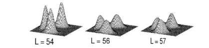
Figure 18: Many-particle energy spectrum (the interaction energy) for 4 electrons in a harmonic confinement as a function of the angular momentum. Solid points: Exact diagonalization; Squares: Model Hamiltonian (the numbers indicate the vibrational state in question). The lower panel shows the pair correlation functions for some yrast states.

The pair correlation functions shown in the lower panel of Fig. 18 further support this conclusion. For the cusp states (as here at $L=50,54,58$ for $N=4$), the pair correlations show clearly the localization of the electrons in a square geometry, while the points in between these angular momenta reflect the properties of the two different vibrational states.

Finally, let us discuss how this relates to the fractional quantum Hall effect. Laughlin [18] showed already in his pioneering work that the maximum amplitude of the many-electron state in the fractional QHL

$$\Psi_{q}(z_{1},z_{2},\cdots,z_{N})=\prod_{i<j}^{N}(z_{i}-z_{j})^{q}e^{-\sum|z_{k}|^{2}/2\ell_{h}^{2}},$$ (17)

is obtained when the electrons are localized at their classical equilibrium positions. In the wave funtion above, $q$ is an odd integer (the filling fraction of the LLL is $\nu=1/q$). The localization becomes more pronounced when $q$ increases [111]. In the region where the true Wigner crystal is formed, the above wave function is not any more accurate. In small systems, however, already in the region of $\nu=1/3$ ($q=3$) the exact energy spectrum shows the periodic oscillation of the yrast spectrum caused by the electron localization (see Fig. 17). The spectrum in Fig. 18 is from the region $\nu\sim 1/9$.

The classical geometry of the localized electrons depends on their number [117]. Generally, the electrons tend to form concentric rings. Up to five electrons they form a single ring, but for six electrons the ground state is a five-fold ring with one electron at the center, as schematically shown in Fig. 19. This figure displays the classical equilibrium positions, for the example of six (upper panel) and ten electrons (lower panel), respectively (after Bolton and Rössler [118]. See also the discussion in Ref. [4]).

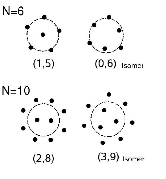
Figure 19: Classical electron positions for small particle numbers, $N\leq 10$, in a parabolic well. After Bolton and Rössler [118].

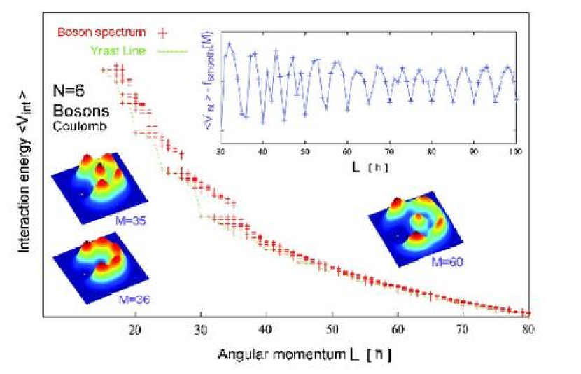
Figure 20: Interaction energy of $N=6$ bosons as a function of the angular momentum. The inset shows the yrast line with a smooth function of angular momentum (3rd order polynomial) subtracted from the energies, in order to make the oscillations more visible. The large-$L$ limit is dominated by a regular oscillation with $\Delta L=5$. The pair correlation functions to the left clearly demonstrate localization in Wigner molecule geometries at high angular momenta. While at smaller $L$-values, the $(1,5)$ and the $(0,6)$ configurations compete, at extreme angular momenta fivefold symmetry dominates.

The localization caused by the highly rotational state is not limited to electrons in a harmonic confinement, but is a more general phenomenon to occur for all particles with long-range interactions. The reason behind is simple: At large angular momenta, the system can be described by the classical rotations and vibrations of Eq. (16). The different symmetry requirements can, however, select different allowed vibration modes for fermions and bosons (at a given angular momentum).

Fig. 20 shows as an example the interaction energy as a function of the angular momentum, for six bosons interacting by Coulomb repulsion. Subtracting a smooth function of angular momentum (3rd order polynomial) from the yrast line, pronounced and regular oscillations of period $\Delta L=5$ are visible in the large-$L$ limit, originating from the localization into a five-fold ring with one boson at the center, just as for the fermion case discussed above. This localization is confirmed by the pair correlations, shown as an inset in the same figure. Reimann et al. [119] have furthermore shown, that the energy spectra of small numbers of bosons and fermions are nearly identical at high angular momenta.

The Laughlin wave function, Eq. (17), is also applicable for bosons. In this case, naturally the exponent $q$ needs to be even. This suggests that there is a relation between the boson and fermion wave functions. Since the boson wave function is symmetric, a proper fermion wave function can be constructed by multiplying the boson wave function with the determinant $\prod(z_{i}-z_{j})$. Indeed, for the wave functions at large angular momenta this construction gives excellent approximations for the fermion wave functions. The overlap between this construction and the exact fermion wave function for four electrons at high angular momenta is typically 99 %  [120]. Note, that this is not only true for the rigidly rotating states, but also for states with internal vibrations.

Why does the rotational motion localize the particles in a harmonic confinement? In the case of electrons with long-range Coulomb interactions one could think that this is caused by Wigner crystallization. When the angular momentum increases, the electron cloud expands due to the centrifugal force and eventually, Wigner crystallization sets in. However, we have already seen that the external magnetic field increases the strength of the confinement. In fact, the average electron density remains essentially constant when localization occurs.

6.4 Vortices in polarized fermion systems

Vortex formation in type-II superconductors is a well-known phenomenon [121]. When the magnetic field increases, at the first critical field strength at a given temperature, vortices penetrate the superconductor forming a regular triangular lattice. Similarly, in rotating ³He vortex formation has been observed by optical measurements [122]. Vortex formation in rotating systems has been considered as a definite signature of superfluidity.

In the case of semiconductor quantum dots, vortex formation was discussed theoretically by Saarikoski et al. [108] using the current-density functional formalism. Later this was confirmed by exact diagonalization calculations [123, 124]. The vortices appeared when the magnetic field was increased beyond formation of the maximum density droplet, but at field strengths below those where the fractional QHL occurs.

Just as for localization of the electrons, as discussed above, in mean-field theory the vortices are visible directly as distinct minima in the total electron density, with the electron current showing circulation of the vortex core, as illustrated in Fig. 21. The vortices seem to localize a in a regular ’molecule’, with geometries resembling those observed for the finite-size Wigner crystallites discussed above.

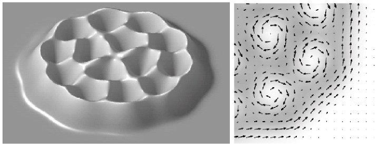
Figure 21: Electron density of a 24 electron quantum dot showing 14 vortices (left) and the corresponding currents (right). Results from a current-spin-density functional calculation by Saarikoski et al. From Ref. [108].

To analyze the vortex solutions gained by the exact diagonalization method, is not an easy task [125]. Naturally, for the exact solution of the many-body Hamiltonian, the total density is circularly symmetric and one has to study correlation functions – just as explained above for the case of Wigner localization. Figure 22 shows the electron-electron pair correlation for 36 electrons at a highly rotational state. Clearly, in addition to the exchange-correlation hole around the reference electron, there are four distinct minima in the pair correlation. These are four localized vortices – the reference electron pins their position, making them visible.

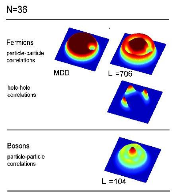
Figure 22: Pair correlation functions calculated for 36 electrons. The upper panel shows the electron-electron correlations for the MMD, $L=630$ (left), for particles at $L=706$ showing four vortices (right), and for holes at the same angular momentum (lower right). The lower panel shows the corresponding correlation function for a bosonic four-vortex state at angular momentum $L=104$. (Note the absence of the exchange hole in the bosonic case.) From Ref. [125].

Other ways to observe the internal symmetry breaking in the exact diagonalization study are to break the circular symmetry, for example by an ellipsoidal confinement [126, 127], or by using perturbation theory [123]. The electron density at the vortex core is zero, and the phase of the wave function changes by $2\pi$ when a coordinate is rotated around the vortex core. In the case of the many-particle wave functions, these characteristics are difficult to use. It was suggested by Saarikoski et al. [108] to determine the phase change of the many-particle wave function by by fixing the positions of $N-1$ coordinates when the $N$’th coordinate is rotated around the vortices (fixing the other coordinates fixes also the positions of the vortices). The phase maps created in this way [108, 123] show that in addition to the ’free’ vortices there is one vortex attached to each electron. In the language of the QHL, each electron carries a flux quantum (in the case of fractional QHL with filling factor $\nu=1/3$, each electron carries three flux quanta). Electrons with attached flux quanta (or vortices) are also called composite fermions [128].

In the polarized case, there is a simple way to understand the occurrence of free vortices. They are holes in the otherwise filled Fermi see, i.e. holes in the MDD, where all states up to the single-particle angular momentum $L_{\rm MDD}=N(N-1)/2$ are filled. When the angular momentum is increased we create holes (missing electrons) corresponding to small angular momenta relative to $L_{\rm MDD}$. Formally, we can can define the creation (annihilation) operator of a hole as $d^{+}=c$ ($d=c^{+}$) and write the Hamiltonian Eq. (15) in terms of these,

$$H=\sum_{i}m_{i}\hbar\omega_{0}(1-d_{i}^{+}d_{i})+2\sum_{i,j,k}\left(V_{ijkj}-V_{ijjk}\right)d_{k}^{+}d_{i}+\sum_{i,j,k,l}V_{ijkl}d_{l}^{+}d_{k}^{+}d_{j}d_{i}+{\rm constant}.$$ (18)

Note, that the interactions between the holes are the same as those between the particles, but the second term means that the particles do not any longer move in a strictly harmonic confinement. Naturally, the solution of this Hamiltonian leads to an equivalent result as that of the original Hamiltonian, requiring the same computational effort.

We will now show that – even within a limited single-particle space – the holes localize to a Wigner molecule. Let us consider $n$ holes in a system with $N$ electrons and restrict the single-particle basis to its minimum possible value in the LLL, i.e. the maximum single-particle angular momentum being $l_{\rm max}=N+n-1$. When the angular momentum of the electron system is $L_{e}=L_{\rm MDD}+\Delta L$, the angular momentum of the system of holes is $L_{h}=(N+n)(N+n-1)-L_{e}=2nN+n(n-1)-\Delta N$. For example, for the $N=4$ particle system (cf. Fig. 22), $L_{h}=66$ corresponds to such high angular momentum that the quasi-particles (now holes) are well localized.

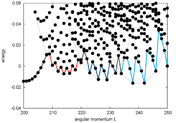
Figure 23: Energy spectrum as function of the total angular momentum for 20 electrons. A smooth function is subtracted from the total energy to show the oscillations of the yrast line (thick line). The thin lines show the lowest energy states with 1, 2, 3, and 4 vortices.

This localization suggests that the excitation spectrum can be determined from the “classical” rotations and vibrations, resulting in similar periodic oscillations as found above for localized electrons at high angular momenta. This indeed is the case, as shown by Manninen et al. [124, 125]. Figure 23 shows the energy spectrum for 20 electrons as a function of angular momentum. The yrast-line shows oscillations, in the beginning with period 2, followed by oscillations of period 3 and then period 4 (in units of angular momentum). These regions correspond to the formation of two, three, and four vortices, respectively. This means that the main features of the many-particle spectrum at these angular momenta are determined by the rotation-vibration spectrum of localized vortices. In Section 6.5 we will see that similar oscillations reveal the existence of vortices in rotating boson systems.

Like for fermions, also in the bosonic case, the structure of the bosonic wave function can be understood in terms of Laughlin-type wave functions [123, 125]. The simplest Ansatz for the single vortex at the center is the Bertsch-Papenbrock [129] wave function

$$\Psi_{\rm 1v}=\prod_{i}(z_{i}-z_{0})\Psi_{\rm MDD},$$ (19)

where $z_{0}=\sum z_{i}/N$ is the center-of-mass coordinate. This wave function is a good approximation for the wave function calculated using only the LLL. For example, for 10 electrons the overlap between these two states is $|\langle\Psi_{\rm 1v}|\Psi_{\rm exact}\rangle|^{2}=0.90$. In a large quantum dot, the center of mass can be approximated as fixed at the origin. Similarly, having $n$ vortices in a ring, we can approximate the wave function as

$$\Psi_{kV} = \prod_{j_{1}}^{N}(z_{j_{1}}-ae^{i\alpha_{1}})\times\cdots\times\prod_{j_{k}}^{N}(z_{j_{k}}-ae^{i\alpha_{k}})\Psi_{MDD}$$ (20)

$$= \prod_{j}^{N}(z_{j}^{k}-a^{n})\Psi_{MDD}~{},$$

where $k$ is the number of vortices, $a$ is the distance of the vortices from the origin and $\alpha_{j}=2\pi j/k$. Clearly, the above wave function does not have a good angular momentum. Projecting to good angular momentum means collecting out states with a given power of $a$. We obtain a state

$$\Psi_{kV}=a^{k(N-K)}{\cal{S}}\left(\prod_{j}^{K}z_{j}^{k}\right)\Psi_{MDD}$$ (21)

which now corresponds to a good angular momentum $M=M_{MDD}+kK$ (here, $\cal{S}$ symmetrizes the polynomial). The above wave function corresponds to the most important configuration of the exact wave function: The $n$ holes are next to each other in consecutive angular momenta. Toreblad et al. [123] called this state a “vortex-generating configuration”. (However, the wave function (21) does not localize the vortices but rather keeps them de-localized at a distance $a$ from the origin).

6.5 Vortices in rotating Bose systems

The observation of Bose-Einstein condensation in atomic traps once again increased the interest in the many-particle physics of the harmonic potential (for a review, see [130]). The experimental observation of vortex lattices in rotating systems was a further milestone. By external fields, the trap can be made to be three-dimensional or quasi-two-dimensional. In a highly rotational state, the cloud of atoms forms a (quasi two-dimensional) disc, with the effective confining potential in the rotating frame being

$$V_{\rm ext}(r,z)=\frac{1}{2}m\omega_{\rm eff}^{2}r^{2}+\frac{1}{2}m\omega_{0}^{2}z=\frac{1}{2}m\left(\omega_{0}^{2}-\omega_{r}^{2}\right)r^{2}+\frac{1}{2}m\omega_{0}^{2}z$$ (22)

where $\omega_{r}$ is the angular velocity of the rotation. For large enough $\omega_{r}$, only the lowest energy state along the $z$-direction is occupied. (Note, that the rotation velocity can not exceed $\omega_{0}$). We can then approximate the rotating Bose system as particles confined in a 2D harmonic trap, and directly compare to fermions confined in a quantum dot.

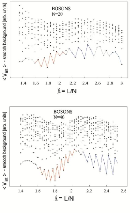
Figure 24: Energy spectrum as function of the total angular momentum for $N=20$ bosons (upper panel) and $N=40$ bosons (lower panel), with Coulomb interactions ($L$ is the angular momentum, $N$ the number of bosons). A smooth function is subtracted from the total energy to show the oscillations of the yrast line (thick line).

The interaction between the atoms in the dilute condensate consists of individual scattering events which are described by the scattering length. The contact interaction, being a standard model interaction for cold atom gases, is written as $v({\bf r}_{i}-{\bf r}_{j})=g\delta({\bf r}_{i}-{\bf r}_{j})$, where $g=4\pi a_{s}\hbar^{2}/m$, $a_{s}$ being the scattering length (for $s$-wave scattering). In the dilute gas, the total energy per particle is proportional to the density. Consequently, in the local density approximation the effective potential will also be proportional to the density. In a Bose system at zero temperature, all particles are in the same quantum state, and the density is simply $\rho({\bf r}=|\psi({\bf r})|^{2}$, where the single-particle wave function $\psi$ is the solution of the so-called Gross-Pitaevskii equation

$$-\frac{\hbar^{2}}{m}\nabla^{2}\psi({\bf r})+\frac{1}{2}m\omega_{0}^{2}r^{2}+g|\psi({\bf r})|^{2}\psi({\bf r})=\epsilon\psi({\bf r}),$$ (23)

which is a mean-field equation in close correspondence to the Kohn-Sham LDA equations for the electron system [131]. The nonlinearity of the equation makes symmetry-breaking possible. Indeed, for a rotating Bose gas, the equation has solutions showing vortex patterns very similar to the ones discussed above for the fermion case [132, 133]. Figure 24 shows the boson spectra, with oscillations in the yrast line resembling to vortex structures as discussed above in the fermion case.

For small numbers of bosons in a harmonic potential, the problem can be solved exactly. In the case of weak interactions between the bosons, the basis set can be restricted to the lowest Landau level. The only difference to the fermion system discussed above is, that now the wave function has to be symmetric. For contact interactions, it has been shown that the Bertsch-Papenbrock Ansatz

$$\Psi_{\rm BP}=\prod_{i}(z_{i}-z_{0})e^{-\sum|z_{k}|^{2}/2\ell_{0}^{2}}=\prod_{i}(z_{i}-z_{0})\Psi_{\rm BEC}$$ (24)

is exact for the state with a single vortex at the center ($\ell_{0}$ is now the oscillator length of the pure confinement). This state has total angular momentum $L=N$. Increasing the angular momentum creates more vortices. A second vortex appears at $L=1.7N$, the third at $L=2.1N$ and the fourth at $L=2.8N$ [133]. An approximation for the $n$ vortices in a ring is again the vortex generating state, Eq. (20), where now the fermion MDD is replaced by the ground state of the BEC. But again, as for fermions, the exact solution is more complicated and supports vortex localization in a much more effective way.

Figure 25: Vortex-vortex correlation functions for three vortices in a fermion and boson system with $N=20$ particles. (The difference in total angular momentum is due to the MDD in the fermion case, with $L_{\rm MDD}=N(N-1)/2$). The boson wave function was first transformed to fermion Fock states, as described in the text. The arrows shows the site of the reference vortex.

For bosons, the localization of vortices is not as easily seen in the pair correlations as for fermions – mainly, because the bosonic occupancies in the Fock states make it difficult to interpret the vortices directly as unoccupied states or holes in the MDD (as in the fermion case), as the occupation number is not limited. Nevertheless, for small particle numbers we can transform of the boson wave function to its fermionic equivalent, by multiplying it with the determinant $\prod(z_{i}-z_{j})$. Figure 25 shows the vortex-vortex pair correlations determined in this way, for $N=20$ bosons with three vortices ($L=48$). For comparison, the corresponding fermion state (which in this case is not the ground state) is shown as well ($L=328$). The correlation functions appear suprisingly similar.

The above analysis showed very clearly that vortex localization occurs both in the bosonic and the fermionic case, and is mapped out very directly by studying the corresponding correlation functions. The rotational spectra confirmed this observation.

Figure 24 shows the energetically low-lying many-body energies for $N=20$ and 40 bosons, respectively. As for fermions, we observe the oscillatory behavior of the yrast line. We saw above that the period of the oscillations corresponds to the number of the first few vortices that localize on a ring. Note, that on the horizontal axis we have now given the ratio $L/N$ in order to demonstrate that for bosons, the regions for different vortex numbers only depend on $L/N$. This is not the case in fermion systems [125], where for larger systems with $N\geq 14$, the vortices appear closer of the surface of the MDD, leaving its center unaffected.

Finally, we mention the possibility of vortex formation in boson and fermion systems where the particles have an internal degree of freedom, like spin or pseudospin. In this case, the single-component vortex patterns are still observed, however, they are not any longer lowest-energy excitations. This holds for fermions [134] as well as for bosons.

Concluding our discussion of vortices in harmonically confined quantum systems that are set rotating, we should emphasize that the vortex formation gives characteristic oscillations in the yrast spectrum [125]. The low-energy states of the rotational spectrum are determined by the rigid rotation and vibrational states of Wigner molecules of vortices [124]. The vortex formation is similar for bosons and fermions and it is nearly independent of the form of the repulsive interparticle interaction [123, 135].

7 One-dimensional systems

7.1 1D harmonic oscillator

Let us finally discuss interacting electrons confined by a one-dimensional harmonic oscillator, as well as a quasi-one-dimensional quantum ring. In an anisotropic oscillator, $V_{\rm ext}=(1/2)m(\omega_{x}^{2}x^{2}+\omega_{y}^{2}y^{2}+\omega_{z}^{2}z^{2})$ choosing the frequencies $\omega_{y}$ and $\omega_{z}$ of two spatial directions is so large that the particles occupy only the lowest state in the perpendicular direction, the system becomes effectively one-dimensional.

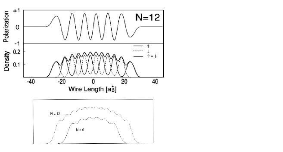
Figure 26: Upper figure: Spin polarization, as well as spin- and total electron densities at the center of a quasi-1D wire with 12 electrons, calculated with the LSDA. Lower figure: Electron densities for $N=6$ and $N=12$ noninteracting spinless fermions in a 1D harmonic oscillator.

The 1D system of fermions is very different from the 2D and 3D cases. The exchange interaction, or the Pauli exclusion principle, becomes dominating. Since two electrons with the same spin can not be in the same place, in 1D this means that electrons with the same spin can not pass each other. This enhances drastically the tendency to form a spin density wave. In fact, an infinite 1D electron gas is unstable against the so-called spin-Peierls transition: A static spin density makes a spin-dependent mean-field potential (e.g. LSDA) with a wave length of $\pi/2k_{F}$ and consequently opens a gap at the Fermi level. (Remember that the Fermi surface consist of only two points in 1D). Figure 26 shows the result of an LSDA calculation for 12 electrons in a quasi-1D harmonic potential, showing very clearly the resulting spin-density wave. The total density shows 12 maxima corresponding to ’localized’ electrons forming an anti-ferromagnetic chain. Even in 1D, the LSDA can not properly localize the electrons.

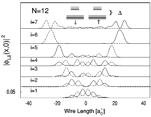
Figure 27: Single-particle (Kohn-Sham) densities and energy eigenvalues (inset) for a linear finite wire with 12 electrons. Note that the last occupied state ($i=6$) is localized at either end of the wire. The energy gap between occupied and unoccupied states is denoted by $\Delta$ in the inset. From Ref. [64].

It is interesting to compare the self-consistent electron density to that of non-interacting electrons, shown also in Fig. 26. The density for 12 spinless electrons is quite similar to the LSDA result, while the density of 12 electrons with spin has only 6 maxima since each single-particle state now occupies two electrons. However, the similarity of the LSDA density to that of the noninteracting spinless electrons does not reach to the individual single-particle wave functions. Figure 27 shows the densities of the single-particle wave functions of the LSDA calculation. Interestingly, the last occupied state $i=6$ is localized at the end of the electron cloud. This end state is related to the surface states in a metal surface. The existence of the periodic potential which ends at the surface makes localized states possible [41]. In our 1D case the periodic potential is provided by the spin-Peierls transition and the static spin-density wave.

7.2 Quantum rings

The observation of Aharonov-Bohm oscillations [136] and persistent currents [137] have made quasi-1D quantum rings a playground for simple theories. Indeed, the one-dimensionality as such gives a multitude of interesting properties [138, 87]. Here we will only study the spectral properties of finite rings since they are directly related to what we discussed earlier in connection to rotational states in a 2D harmonic confinement.

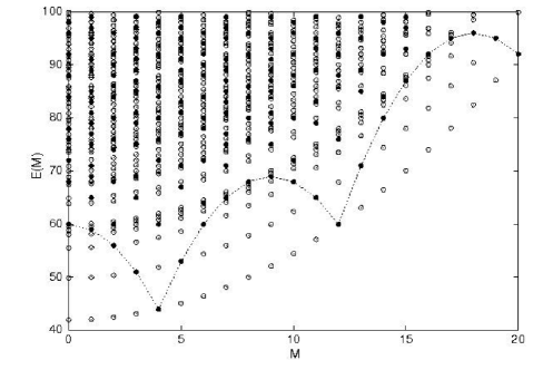
Figure 28: Many-particle energy spectrum of 8 non-interacting polarized electrons in a strictly one-dimensional quantum ring (black dots) compared to the rotation-vibration spectrum of classical particles interacting with $1/r^{2}$ interaction (open circles). The dotted curve shows the yrast line of the polarized electrons. From Ref. [87].

In the strictly 1D case, the single-particle eigenvalues are $\epsilon_{l}=\hbar^{2}l^{2}/2mR^{2}$, where $R$ is the radius of the ring and $l$ the angular momentum eigenvalue. The corresponding single-particle states are $\psi(\phi)=\exp(il\phi)$. The total angular momentum and energy for noninteracting particles is

$$L=\sum_{i}^{N}l_{i},\qquad E=\sum_{i}^{N}\epsilon_{l_{i}}.$$ (25)

Let us first consider noninteracting polarized (spinless) fermions. It is easy to determine their energy as a function of the total angular momentum using Eqs. (25). The results are shown for $N=8$ fermions in Fig.28 as black dots. The yrast line shows a period of eight, suggesting that the electrons are localized in an octagon, the downward cusps corresponding to purely rotational states of the octagon. The black dots correspond to internal vibrations of the Wigner molecule. The fact that noninteracting polarized electrons form a Wigner molecule is a special property of 1D. It can be shown that particles interacting with $1/r^{2}$ interaction in a 1D ring have the same energy spectrum as noninteracting particles (or particles interacting with an infinitely strong interaction of delta-function type) [87]. Figure 28 shows (as open circles) also the classically determined energies

$$E=E_{\rm rot}+E_{\rm vib}=\frac{\hbar^{2}L^{2}}{2NmR^{2}}+\sum_{\nu}n_{\nu}\hbar\omega_{\nu}$$ (26)

for the $1/r^{2}$ interaction. Each vibrational level forms a rotational band. We can see that the spectrum of noninteracting polarized fermions (black dots) consists only of points at the classical energies. In fact, for electron with spin and infinite strong delta-function interaction ($v(r)=A\delta(r)$, where $A\rightarrow\infty$) one obtains all the classical points (open circles).

The reason why noninteracting spinless electrons localize and have vibrational modes simply follows from the fact that the electrons can not pass each other. If the electron-electron distance is $d$, each electron is then localized between its neighbors in a region $2d$. Its kinetic energy will then be proportional to $1/d^{2}$. This effectively leads to a $1/r^{2}$ interaction between the electrons.

Interacting electrons in 1D systems have been extensively studied using the Hubbard model (for reviews see [138, 87]). The energy spectrum can be solved exactly using the Bethe Ansatz [139]. There, several analytic results exist. For a half-filled Hubbard band (with one electron per site) it is rather easy to show that the large $U$-limit the Hubbard model becomes an anti-ferromagnetic Heisenberg model. However, the Heisenberg model seems to be a good approximation also for small filling [140, 87]. This is important, since the low-filling limit of the Hubbard model approaches to free electrons with delta interaction (this is the same as the tight-binding model approaching the free electron model at the bottom of the band [141]). Thus, also free electrons with spin localize in anti-ferromagnetic order as long as they have strong enough repulsive interactions between them.

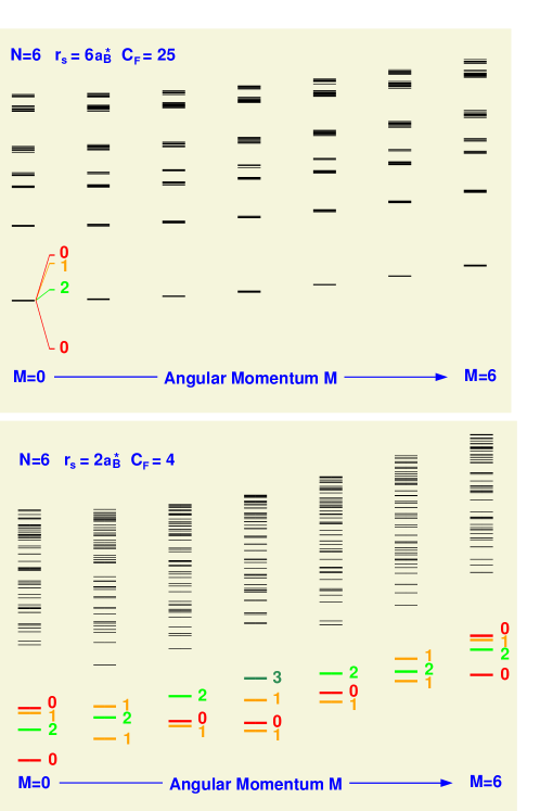
Figure 29: Energy spectra for two quasi-one-dimensional continuum rings with six electrons (in zero magnetic field). The upper panel is for a narrow ring and it shows several vibrational bands. The lower panel is for a wider ring which shows stronger separation of energy levels corresponding to different spin states (shown as numbers next to the energy levels). Note that also the narrow ring has the same spin-ordering of the nearly degenerate state as expanded for the lowest $L=0$ state.

Koskinen et al. [142] performed exact diagonalization calculations for electrons confined in a quasi-1D ring described with the external 2D potential $V_{\rm ext}=m\omega_{0}^{2}(r-r_{0})^{2}/2$, where $r=(x,y)$. The rotational spectrum for six particles is shown in Fig. 29 for two different values of the narrowness of the ring. The upper panel corresponds to a very narrow ring. In this case, the different vibrational bands are clearly separated and correspond quantitatively to the energies determined by solving the vibrational frequencies of the classical linear chain of electrons on the ring. The lower panel shows the result obtained for a wider, less one-dimensional ring. In this case, only the vibrational ground state is clearly separated, with the different spin-states separating in energy. With high accuracy, these different spin-states correspond to those of an antiferromagnetic Heisenberg model for six electrons on a ring [142].

In narrow quantum rings the rotational spectrum is very robust. It is insensitive to the interparticle interaction or the specific model for the confinement. Even the discrete Hubbard model gives similar results as the continuum approaches [87]. However, this demonstrates once more that the most clear indication of Wigner molecules in the ground states of high-symmetry systems can be obtained by analyzing the rotation-vibration spectrum.

8 Concluding remarks

In this short review, we summarized some characteristic aspects of finite quantal systems, that have their origin in the quantized level structure in – and beyond – the mesoscopic regime. We discussed shell structure and deformation, as well as the ocurrence of Hund’s rule in finite fermion systems, conjointly for metallic clusters, quantum dots in semiconductor heterostructures, or cold atoms in traps – seemingly different, but nevertheless in many aspects rather similar quantum systems. Like for atoms, shell structure does not only determine the stability and chemical inertness of metallic clusters, but also determines the conductance of a small quantum dot – both close to, and far away from equilibrium.

The experimental realization of Bose-Einstein condensation in an atomic gas [143, 144, 145, 146] opened up a whole new research field on ultra-cold atoms and coherent matter. In a cloud of bosonic atoms that is set rotating, vortices may form. We discussed the fact that this vortex formation is not unique for bosonic systems, but may occur in a very similar way for (non-paired) fermions under rotation, showing many analogies to the physics of the quantum Hall effect. Extreme rotation causes strong correlations, and the system is formally equivalent to charged particles in a strong magnetic field. We finally gave a short summary of the physics of a finite fermionic system in quasi one dimension.

As a final remark, we wish to emphasize that the many analogies existing between nanostructures such as quantum dots and quantum wires, and cold atom gases will become more important in the future – last but not least due to the fact that these systems can be built much more “clean”, and thus more coherent, than their semiconductor counterparts. An example for the cross-fertilization between these different sub-fields of physics, is the recently discussed possibility of of van-der-Waals blockade [147], which is expected to play a key role in transport experiments on confined cold atoms, and in atomtronic devices [148].

9 Acknowldegements

This work was financially supported by the Swedish Research Council and the Swedish Foundation for Strategic Research, as well as uthe European Community project ULTRA-1D (NMP4-CT-2003-505457). We thank J. Akola, M. Borgh, P. Singha Deo, H. Häkkinen, G. Kavoulakis, M. Koskinen, P. Lipas, B. Mottelson, P. Nikkarila, M. Toreblad, S. Viefers, and Y. Yu for their collaboration on the subjects discussed in this review.

References

- [1] Å. Bohr and B. R. Mottelson, 1975, Nuclear Structure (W.A. Benjamin, London 1975).
- [2] W. de Heer, Rev. Mod. Phys. 65, 611 (1993).
- [3] S. Tarucha, D.G. Austing, T. Honda, R.J. van der Haage, and L. Kouwenhoven, Phys. Rev. Lett. 77, 3613 (1996).
- [4] S.M. Reimann and M. Manninen, Rev. Mod. Phys. 74, 1283 (2002).
- [5] J. Akola, M. Manninen, H. Häkkinen, U. Landman, X. Li, and L.-S. Wang, Phys. Rev. B 60, R11297 (1999).
- [6] M. Brack, Rev. Mod. Phys. 65, 677 (1993).
- [7] I. Talmi, Simple models for complex nuclei (Harwood, Chur 1993).
- [8] D. Pfannkuche, and R.R. Gerhardts, Phys. Rev. B 44 13132 (1991).
- [9] A. Wixforth, M. Kaloudis, C. Rocke, K. Ensslin, M. Sundaram, J.H. English and A.C. Gossard, Semicond. Sci. Tech. 9, 215 (1994).
- [10] P. Hawrylak, P.A. Schulz, and J.J. Palacios, Solid State Comm. 93, 909 (1995).
- [11] T. Darnhofer, U. Rössler, and D.A. Broido, Phys. Rev. B 52, 14379 (1995).
- [12] D. Heitmann, K. Bollweg, V. Gudmundsson, T. Kurth, and S.P.Riege, Physica E 1, 204 (1997).
- [13] W. Kohn, Phys. Rep. 123, 1242 (1961).
- [14] S. Frauendorf, V.V. Pashkevich, Z. Phys. D 26, 98 (1993).
- [15] V. Fock, Z. Phys. 47, 446 (1928).
- [16] C. G. Darwin, Proc. Cambridge Philos. Soc. 27, 86 (1930).
- [17] L. Landau, Z. Phys. 64, 629 (1930).
- [18] R.B. Laughlin, Phys. Rev. B 27, 3383 (1983).
- [19] N. D. Lang and W. Kohn, Phys. Rev. B 1, 4555 (1970).
- [20] N.D. Lang, Solid State Phys. 28, 225 (1973).
- [21] M. Manninen, R. Nieminen, P. Hautojärvi, and A. Arponen, Phys. Rev. B 12, 4012 (1975).
- [22] M. J. Puska, R. M. Nieminen, and M. Manninen, Phys. Rev. B 24, 3037 (1981).
- [23] J.L. Martins, R. Car and J. Buttet, Surf. Sci. 106, 265 (1981).
- [24] R. Monnier and J.P. Perdew, Phys. Rev. B 17, 2595 (1978).
- [25] R.G. Parr and W. Yang, Density-functional theory of atoms and molecules (Oxford Universiy Press, Oxford 1989).
- [26] W. Ekardt, Phys. Rev. Lett. 52, 1925 (1984).
- [27] C. Yannouleas, Phys. Rev. B 58, 6748 (1998).
- [28] M. Koskinen, P.O. Lipas, and M. Manninen, Phys. Rev. B 49, 8418 (1994).
- [29] C. Yannouleas, R. A. Broglia, M. Brack, and P.F. Bortignon, Phys. Rev. Lett. 63, 255 (1989).
- [30] J. Martins, R. Car and J. Buttet, Surf. Sci. 106, 261 (1981).
- [31] M. Manninen and R. Nieminen, J. Phys. F 8, 2243 (1978).
- [32] A. Hintermann and M. Manninen, Phys. Rev. B 27, 7262 (1983).
- [33] W. Ekardt, Phys. Rev. B 29, 1558 (1984).
- [34] W.D. Knight, K. Clemenger, W.A. de Heer, W.A. Saunders, M.Y. Chou, and M.L. Cohen, Phys. Rev. Lett. 52, 2141 (1984).
- [35] I.I. Geguzin, Sov. Phys. Solid State 24, 248 (1982).
- [36] B. Mottelson, Nucl. Phys. A 574, 365c (1994).
- [37] R. Balian and C. Bloch, Ann. of Phys. 60, 401 (1970).
- [38] H. Nishioka, K. Hansen and B. Mottelson, Phys. Rev. B 42, 9377 (1990).
- [39] J. Pedersen, S. Bjørnholm, J. Borgreen, K. Hansen, T.P. Martin, and H.D. Rasmunssen, Nature 353, 733 (1991).
- [40] M. Walter and H. Häkkinen, Phys. Chem. Chem. Phys. 8, 5407 (2006).
- [41] A. Zangwill, Physics at Surfaces (Cambridge University Press, Cambridge 1988).
- [42] T.P. Martin, Phys. Reports 273, 201 (1996).
- [43] F. Baletto and R. Ferrando, Rev. Mod. Phys. 77, 371 (2005).
- [44] S. Bjørnholm and J. Borggreen, Phil. Mag. B 79, 1321 (1999).
- [45] F. Chandezon, S. Bjørnholm, J. Borggreen, and K. Hansen, Phys. Rev. B 55, 5485 (1997).
- [46] T.P. Martin, U. Näher, H. Schaber, and U. Zimmermann, J. Chem. Phys. 100, 2322 (1994).
- [47] K. Clemenger, Phys. Rev. B 32, 1359 (1985).
- [48] M. Brack, J. Damgaard, A.S. Jensen, H.C. Pauli, V.M. Strutinsky, and C.Y. Wong, Rev. Mod. Phys. 44, 320 (1972).
- [49] S.M. Reimann, M. Brack, and K. Hansen, Z. Phys. D 28, 235 (1993).
- [50] C. Yannouleas and U. Landman, Phys. Rev. B 48, 8376 (1993).
- [51] S.M. Reimann, S. Frauendorf, and M. Brack, Z. Phys. D 34, 125 (1995).
- [52] S.M. Reimann and S. Frauendorf, Surf. Rev. Lett. 3, 25 (1996).
- [53] Z. Penzar and W. Ekardt, Z. Phys. D 17, 69 (1990).
- [54] T. Hirschmann, M. Brack, and J. Meyer, Annalen der Physik 3, 336 1994.
- [55] M. Manninen, Phys. Rev. B 34, 6886 (1986).
- [56] M. Koskinen, P.O. Lipas, and M. Manninen, Z. Phys. D 35, 285 (1995).
- [57] M. Moseler, B. Huber, H. Hakkinen, U. Landman, G. Wrigge, M.A. Hoffmann, and B. von Issendorff, Phys. Rev. B 68, 165413 (2003).
- [58] H. Häkkinen, J. Kolehmainen, M. Koskinen, P.O. Lipas and M. Manninen, Phys. Rev. Lett. 78, 1034 (1997).
- [59] M. Koskinen, P.O. Lipas, and M. Manninen, Nucl. Phys. A 591, 421 (1995).
- [60] M. Manninen, J. Kolehmainen, M. Koskinen, and S.M. Reimann, Physica Scripta T88, 90 (2000).
- [61] A. Yoshida, T. Dossing, and M. Manninen, J. Chem. Phys. 101, 3041 (1994).
- [62] C. Kohl, B. Montag, and P.-G. Reinhard, Z. Phys. D 38, 81 (1996).
- [63] C. Kohl and P.-G. Reinhard, Z. Phys. D 39, 225 (1997).
- [64] S.M. Reimann, M. Koskinen, J. Helgesson, P.E. Lindelof and M. Manninen, Phys. Rev. B 58, 8111 (1998).
- [65] S.M. Reimann, M. Koskinen, H. Häkkinen, P.E. Lindelof, and M. Manninen, Phys. Rev. B 56, 12147 (1997).
- [66] I. Hamamoto, B.R. Mottelson, H. Xie, and X.Z. Zhang, Z. Phys. D 21, 163 (1991).
- [67] J. Akola, K. Rytkönen, and M. Manninen Eur. Phys. J. D 16, 21 (2001).
- [68] U. Röthlisberger and W. Andreoni, J. Chem. Phys. 94, 8129 (1991).
- [69] J. Li, X. Li, H.J. Zhai, L.S. Wang, Science 299, 864 (2003).
- [70] Th. Diederich, T. Döppner, Th. Fennel, J. Tiggesb umker, and K.-H. Meiwes-Broer, Phys. Rev. A 72, 023203 (2005).
- [71] Y.-P. Chiu, L.-W. Huang, C.-M. Wei, C.-S. Chang, and T.-T. Tsong, Phys. Rev. Lett. 97, 165504 (2006).
- [72] J. Dudek, A. Góźdź, N. Schunck, and M. Miśkiewicz, Phys. Rev. Lett. 88, 252502 (2002).
- [73] J. Dudek, C. Curien, N. Dubray, J. Dobaczewski, V. Pangon, P.Olbratowski, and N. Schunck, Phys. Rev. Lett. 97, 072501 (2006).
- [74] N. Schunck, J. Dudek, A. Góźdź, and P.H. Regan, Phys. Rev. C 69, 061305(R) (2004).
- [75] T. Chakraborty, Quantum Dots: A survey of the properties of artificial atoms (North-Holland, Amsterdam 1999).
- [76] T. Demel, D. Heitmann, P. Grambow, and K. Ploog, Phys. Rev. Lett. 64, 788 (1990).
- [77] B. Tanatar, and D.M. Ceperley, Phys. Rev. B 39, 5005 (1989).
- [78] P. Matagne, J.P. Leburton, D.G. Austing, and S. Tarucha, Phys. Rev. B 65, 85325 (2001).
- [79] C. Thelander, T. Mårtensson, M. T. Björk, B. J. Ohlsson, M. W. Larsson, L. R. Wallenberg and L. Samuelson, Appl. Phys. Lett. 83, 2052, (2003)
- [80] A. Fuhrer, L. E. Fröberg, J. N. Pedersen, M. W. Larsson, A. Wacker, M.-E. Pistol, and L. Samuelson, Nano Letters 7, 243 (2007).
- [81] M. Koskinen, M. Manninen, and S.M. Reiman, Phys. Rev. B 56, 12147 (1997).
- [82] C. Attaccalite, S. Moroni, P. Gori-Giorgi, G.B. Bachelet, Phys. Rev. Lett. 88, 256601 (2002), and Erratum, Phys. Rev. Lett. 91, 109902 (2003).
- [83] M. Borgh, M. Toreblad, M. Koskinen, M. Manninen, S. Åberg and S.M. Reimann, Int. J. of Quant. Chem. 105, 817 (2005).
- [84] S.M. Reimann, M. Koskinen, M., M. Manninen, and B. Mottelson, Phys. Rev. Lett. 83, 3270 (1999).
- [85] K. Hirose, and N.S. Wingreen, Phys. Rev. B 59, 4604 (1999).
- [86] A. Harju, E. Räsänen, H. Saarikoski, M.J. Puska, R.M. Nieminen, K. Niemälä, Phys. Rev. B69, 153101 (2004).
- [87] S. Viefers, P. Koskinen, P.S. Deo, and M. Manninen, Physica E 21, 1 (2004).
- [88] C. Yannouleas and U. Landman, Proc. Nat. Acad. Sci. 103, 10600 (2006).
- [89] E.P. Wigner, Phys. Rev. 46, 1002 (1934).
- [90] D.M. Ceperley, and B.J. Alder, Phys. Rev. Lett. 45, 566 (1980).
- [91] C.E. Creffield, C.E., W. Häusler, J.H. Jefferson, and S. Sarkar, Phys. Rev. B 59, 10719 (1999)
- [92] R. Egger, W. Häusler, C.H. Mak, and H. Grabert, Phys. Rev. Lett. 82, 3320 (1999).
- [93] C. Yannouleas, and U. Landman, Phys. Rev. Lett. 82, 5325 (1999).
- [94] H.M. Müller and S.E. Koonin, Phys. Rev. B 54, 14532 (1996).
- [95] S.M. Reimann, M. Koskinen, and M. Manninen, Phys. Rev. B 62, 8108 (2000).
- [96] D. Pfannkuche, R.R. Gerhardts, P.A. Maksym, and V. Gudmundsson, Physica B 189, 6 (1993).
- [97] M. Taut, J. Phys. A 27, 1045 (1994).
- [98] M. El-Said, Phys. Status Solidi B193, 105 (1996).
- [99] A. González, L. Quiroga, and B.A. Rodriguez, Few-Body Syst. 21, 47 (1996).
- [100] M. Dineykhan, and R.G. Nazmitdinov, Phys. Rev. B 55, 13707 (1997).
- [101] J.-L. Zhub, S. Zhub, Z. Zhuc, Y. Kawazoec and T. Yaoc, Phys. Lett. A 246, 157 (1998).
- [102] K. Kärkkäinen, M. Koskinen, S.M. Reimann, and M. Manninen, Phys. Rev. B 70, 195310 (2004).
- [103] T.H. Oosterkamp, J.W. Janssen, L.P. Kouwenhoven, D.G. Austing, T. Honda, and S. Tarucha, Phys. Rev. Lett. 82, 2931 (1999).
- [104] K. Capelle and G. Vignale, Phys. Rev. B 65, 113106 (2002).
- [105] R. D’Agosta and G. Vignale, Phys. Rev. B 71, 245103 (2005).
- [106] G. Vignale and M. Rasolt, Phys. Rev. Lett. 59, 2360 (1987).
- [107] M. Koskinen, J. Kolehmainen, S.M. Reimann, J. Toivanen, and M. Manninen, Eur. J. Phys. D 9, 487 (1999).
- [108] H. Saarikoski, A. Harju, M. J. Puska, and R. M. Nieminen, Phys. Rev. Lett. 93, 116802 (2004).
- [109] E. Goldmann and S.R. Renn, Phys. Rev. B 60, 16611 (1999).
- [110] M. Toreblad, Y. Yu, S.M. Reimann, M. Koskinen, and M. Manninen, J. of Phys. B: At. Mol. & Opt. 39, 2721 (2006).
- [111] M. Manninen, S. Viefers, M. Koskinen, and S. M. Reimann, Phys. Rev. B 64, 245322 (2001).
- [112] J.R. Grover, Phys. Rev. 157, 832 (1967).
- [113] P.A. Maksym, Phys. Rev. B 53, 10871 (1996).
- [114] P.A. Maksym, H. Imamura, G.P. Mallon, and A. Aoki, J. Phys. Cond. Mat. 12, R299 (2000).
- [115] J.-P. Nikkarila and M. Manninen, Solid State Commun. 141, 209 (2007).
- [116] M. Tinkham, (McGraw-Hill, New York 1964).
- [117] V.M. Bedanov and F.M. Peeters, Phys. Rev. B 49, 2667 (1994).
- [118] F. Bolton, and U. Rößler, Superlatt. Microstr. 13, 139 (1993).
- [119] S.M. Reimann, M. Koskinen, Y. Yu, and M. Manninen, New J. Phys., 8, 59 (2006).
- [120] M. Borgh, M. Manninen and S.M. Reimann, to be published.
- [121] M. Tinkham, Introduction to Superconductivity, (Krieger Pub Co 1975).
- [122] A. J. Manninen, J. P. Pekola, G. M. Kira, J. P. Ruutu, A. V. Babkin, H. Alles, and O. V. Lounasmaa, Phys. Rev. Lett. 69, 2392 (1992).
- [123] M. Toreblad, M. Borgh, M. Manninen, M. Koskinen, and S.M. Reimann, Phys. Rev. Lett. 93, 090407 (2004).
- [124] M. Manninen, S. M. Reimann M. Koskinen, Y. Yu, and M. Toreblad, Phys. Rev. Lett. 94, 106405 (2005).
- [125] S.M. Reimann, M. Koskinen, Y. Yu, and M. Manninen, Phys. Rev. A 74, 043603 (2006).
- [126] M. Manninen, M. Koskinen, S.M. Reimann, and B. Mottelson, Eur. Phys. J. D 16, 381 (2001).
- [127] H. Saarikoski, S. M. Reimann, E. Räsänen, A. Harju, and M. J. Puska, Phys. Rev. B 71, 035421 (2005).
- [128] J.K. Jain, and R.K. Kamilla, in Composite Fermions: A unified view of the quantum Hall effect, edited by O. Heinonen (World Scientific, River Edge, NJ, 1998).
- [129] G.F. Bertsch and T. Papenbrock, Phys. Rev. Lett. 83, 5412 (1999).
- [130] C.J. Pethick, and H. Smith, Bose-Einstein condensation in dilute gases. (Cambridge University Press, Cambridge, 2002).
- [131] K. Capelle et al., to be published (2007).
- [132] D.A. Butts and D.S. Rokshar, Nature (London) 397, 327 (1999).
- [133] G.M. Kavoulakis, B. Mottelson and C.J. Pethick, Phys. Rev. A 62, 063605 (2000).
- [134] M. Koskinen, S.M. Reimann, J.-P. Nikkarila, and M. Manninen, J. Phys.: Condens. Matter 19, 076211 (2007).
- [135] O.K. Vorov, M.S. Hussein, and P. van Isacker, Phys. Rev. Lett. 90, 200402 (2003).
- [136] Y. Aharonov and D. Bohm, Phys. Rev. 115, 485 (1959).
- [137] R. A. Webb, S. Washburn, C. P. Umbach, and R. B. Laibowitz, Phys. Rev. Lett. 54, 2696 (1985).
- [138] E.B. Kolomeisky, and J.P. Straley, Rev. Mod. Phys. 68, 175 (1996).
- [139] E.H. Lieb and F.Y. Wu, Phys. Rev. Lett. 20, 1445 (1968).
- [140] N. Yu and M. Fowler, Phys. Rev. B 45, 11795 (1992).
- [141] M. Manninen, J. Mansikka-aho, and E. Hammarén, Europhys. Lett. 15, 423 (1991).
- [142] M. Koskinen, M. Manninen, B. Mottelson, and S.M. Reimann, Phys. Rev. B 63, 205323 (2001).
- [143] M.H. Anderson, J.R. Ensher, M. R. Matthews, c.E. Wieman and E.A. Cornell, Science 269, 189 (1995).
- [144] K.B. Davis, M.O. Mewes, M.R. Andrews, N.J. van Druten, D.S. Drufee, D.M. Kurn and W. Ketterle, Phys. Rev. Lett. 75, 3969 (1995).
- [145] W. Ketterle, Rev. Mod. Phys. 74, 1131 (2002).
- [146] E. A. Cornell and C. E. Wieman, Rev. Mod. Phys. 74, 875 (2002).
- [147] K. Capelle, M. Borgh, K. Kärkkäinen and S.M. Reimann, http://arxiv.org/cond-mat/0702246 to be published (2007).
- [148] B. T. Seaman, M. Krämer, D. Z. Anderson and M. J. Holland, http://arxiv.org/cond-mat/0606625 (2006).