Electron Transport through Nanosystems Driven by Coulomb Scattering

Abstract

Electron transmission through nanosystems is blocked if there are no states connecting the left and the right reservoir. Electron-electron scattering can lift this blockade and we show that this feature can be conveniently implemented by considering a transport model based on many-particle states. We discuss typical signatures of this phenomena, such as the presence of a current signal for a finite bias window.

I Introduction

Quantum dots constitute an excellent testbed for transport through general nanosystems, where the local density of states is dominated by discrete localized levels. The key points are conduction quantization van Wees et al. (1988) due to the discreteness of levels, Coulomb Blockade due to electron repulsion,Meirav et al. (1990) and the interplay between resonant tunneling and charging in double dot structures.van der Wiel et al. (2003) In this work we consider a further issue, the transport by electron-electron scattering.

Electron-electron scattering is not included in standard transmission models,Lindsay and Ratner (2007) where the Coulomb interaction is taken into account by a mean-field approach frequently including exchange-correlation interactions as well. Within such models electron transport strongly depends on the presence of states in the system connecting both leads.Heurich et al. (2002) Here we show that electron-electron scattering allows for additional transport channels and that it can be consistently implemented using a many-particle basis following the concepts developed in Refs. Kinaret et al., 1992; Pfannkuche and Ulloa, 1995; Tanaka and Akera, 1996; Hettler et al., 2003; Pedersen and Wacker, 2005; Muralidharan et al., 2006.

While in double-dot structures, each dot has direct access to a reservoir with a continuous level density, the situation is essentially different in triple-dot structures,Gaudreau et al. (2006) where the states in the central dot only couple to discrete states in the neighboring dots. Thus the properties of these states are far more sensitive to scattering events, which may essentially determine the transport through the structure. This is precisely the situation depicted in Fig. 1: Here the upper level 4 of the middle dot can be filled from the left lead by resonant tunneling via level 1, while its lower level can be emptied into the right lead by resonant tunneling via level 6. Thus the current is very sensitive to scattering between level 4 and level 3. In this work we restrict to electron-electron scattering, which is appropriate if the phonon energies do not match the transition energy.

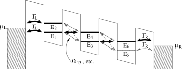
Figure 1: The triple-dot system considered. The bold lines represent the simplified system.

II The Model

II.1 The System

The system depicted in Fig. 1 is described by the Hamiltonian $\hat{H}=\hat{H}_{\mathrm{dots}}+\hat{H}_{\mathrm{leads}}$:

$$\hat{H}_{\mathrm{dots}}=\sum_{i=1}^{6}E_{i}a_{i}^{\dagger}a_{i}-\sum_{ij}\Omega_{ij}a_{i}^{\dagger}a_{j}+\hat{H}_{\mathrm{ee}}$$ (1)

refers to the dot region where $a_{i}^{\dagger}$ ($a_{i}$) is the creation (annihilation) operator for the $i$’th state. Assuming that the states in the individual dots are strongly localized, only states in dots next to each other couple and we restrict to those couplings $\Omega_{ij}$ depicted in Fig. 1. For the Coulomb part $\hat{H}_{\mathrm{ee}}$ we neglect interactions between the leads and the dots as well as interactions between next-nearest neighboring dots. Then we obtain

$$\hat{H}_{\mathrm{ee}}=U(a_{1}^{\dagger}a_{2}^{\dagger}a_{2}a_{1}+a_{3}^{\dagger}a_{4}^{\dagger}a_{4}a_{3}+a_{5}^{\dagger}a_{6}^{\dagger}a_{6}a_{5})\\ +U_{\mathrm{n}}(a_{1}^{\dagger}a_{1}+a_{2}^{\dagger}a_{2}+a_{5}^{\dagger}a_{5}+a_{6}^{\dagger}a_{6})(a_{3}^{\dagger}a_{3}+a_{4}^{\dagger}a_{4})\\ +\{U_{\mathrm{sc}}a_{3}^{\dagger}a_{2}^{\dagger}a_{1}a_{4}+U_{\mathrm{sc}}a_{5}^{\dagger}a_{4}^{\dagger}a_{3}a_{6}+h.c.\}\,.$$ (2)

Here $U$ and $U_{\mathrm{n}}$ are the matrix elements of the standard Coulomb repulsion between states located in the same and neighboring dots, respectively. $U_{\mathrm{sc}}$ describes Coulomb scattering between different states, which is the central issue of this work.foo

Finally, the Hamiltonian of the leads and their coupling to the dots reads:

$$\hat{H}_{\mathrm{leads}}=\sum_{k\ell}E_{k\ell}c_{k\ell}^{\dagger}c_{k\ell}-\sum_{ik\ell}\left(t_{ik\ell}a_{i}^{\dagger}c_{k\ell}+t^{*}_{ik\ell}c^{\dagger}_{k\ell}a_{i}\right)$$ (3)

Here $\ell=L,R$ denotes the left and right lead, respectively. The energies $E_{k\ell}$ in lead $\ell$ provide a continuum of states (labeled by $k$). We assume that the corresponding density of states has the constant value $g_{\ell}$ in the energy range $-W<E<W$ and is zero otherwise. Disregarding the $k$-dependence of the tunneling matrix elements $t_{ik\ell}$ we set $t_{1kL}=t_{2kL}=\sqrt{\Gamma_{L}/(2\pi g_{L})}$ and $t_{5kR}=t_{6kR}=\sqrt{\Gamma_{R}/(2\pi g_{R})}$. These are the transitions sketched in Fig. 1. All other tunneling matrix elements are neglected in Eq. (3). Throughout this work we restrict to a single spin direction for simplicity.

II.2 Parameters

For specific calculations we use the parameters of Table 1 unless stated otherwise.

$E_{1}=40$	$E_{2}=60$	$E_{3}=20$	$E_{4}=40$	$E_{5}=0$	$E_{6}=20$
$\Omega_{14}=\Omega_{36}=\Omega_{23}=\Omega_{45}=0.1$				$\Omega_{13}=\Omega_{35}=0.05$
$\Gamma_{L}=\Gamma_{R}=0.1$		$\mu_{L}=50$	$\mu_{R}=10$	$\Omega_{24}=\Omega_{46}=-0.2$
$U_{\mathrm{sc}}=-0.2$	$U=10$	$U_{\mathrm{n}}=3$	$k_{B}T=2$	$W=400$

Table 1: Parameters used if not stated otherwise. They refer to the modulated nanowire discussed in Sec. II.2, but have been rounded off for an easier recognition of scales in the plots. All energies are in meV. In the simplified system we neglect level 5 and set $\Omega_{13}=\Omega_{24}=\Omega_{23}=\Omega_{46}=U=U_{\mathrm{n}}=0$.

They relate to an InAs/InP modulated nanowire structure similar to the structures of Refs. Björk et al., 2002; Fuhrer et al., 2007. We assume three InAs wells with a thickness of $40$ nm, which are separated by $3$ nm thick InP barriers. The outer barriers are assumed to be $1.5$ nm thick. As we are only interested in order of magnitude estimates we choose the simple one-band envelope function model, with Dirichlet boundary condition on the outside of the wire. In addition, we assume that the wire is cylindrical with radius $R=20$ nm which enables us to reduce the problem to a one dimensional problem by using cylindrical coordinates, i.e., the single particle Hamiltonian is given by

$$H=[-\frac{\partial}{\partial z}\frac{\hbar^{2}}{2m_{\rm eff}}\frac{\partial}{\partial z}+\frac{\hbar^{2}j_{ln}^{2}}{2m_{\rm eff}R^{2}}+V_{c}(z)]$$ (4)

where $j_{ln}$ is the $n$’th zero of the Bessel function $J_{l}$. $m_{\rm eff}$ is the effective mass function, $V_{\rm eff}$ is the conduction band edge function (they are stepwise constant). In the previous section we assumed that states in individual dots are strongly localized. One way of achieving that is to use Wannier states $\Psi_{i}(z)$ for individual dots, assuming a periodic repetition of the structure. Using the masses $m_{\rm InAs}=0.026m_{e}$ and $m_{\rm InP}=0.08m_{e}$, where $m_{e}$ is the free electron mass, and a conduction band offset of $0.6eV$ Björk et al. (2002) we get an energy difference between the ground state and the first excited state of $E_{2}-E_{1}=21$ meV for a given $l$ and $n$. The excitation energy for the radial modes $\tfrac{\hbar^{2}}{2m_{\rm eff}R^{2}}(j_{11}^{2}-j_{01}^{2})=29$ meV is larger and thus these radial modes can be neglected. (In addition, the coupling between states of different radial symmetry should be small.) The couplings $\Omega_{ij}$ are evaluated following Sec. 2.3 of Ref. Wacker, 2002 for a bias drop of 20 meV per period.

For the coupling to the leads we use the estimateWacker and Hu (1999)

$$\Gamma_{iL/R}\approx\frac{2dT_{i}^{2}}{\hbar\sqrt{2(E_{i}-E_{r})/m_{\rm InAs}}},$$ (5)

where $T_{i}$ is the coupling element between Wannier state $i$ in neighboring dots for a barrier width of $1.5$ nm (the outer barrier) and $E_{r}$ is the sum of the conduction band edge of InAs and the radial confinement energy.

In general the Coulomb interaction is described by

$$\hat{H}_{ee}=\frac{1}{2}\sum_{ijkl}U_{ijkl}a_{i}^{\dagger}a_{j}^{\dagger}a_{k}a_{l}$$ (6)

with

$$U_{ijkl}=\int{\rm d}^{3}r\int{\rm d}^{3}r^{\prime}\frac{e^{2}\quad\varphi^{*}_{i}({\bf r})\varphi_{l}({\bf r})\varphi^{*}_{j}({\bf r}^{\prime})\varphi_{k}({\bf r}^{\prime})}{4\pi\epsilon_{r}\epsilon_{0}|{\bf r}-{\bf r}^{\prime}|}$$ (7)

Commonly, one focuses on the direct interaction of two states, where $i=l$ and $j=k$. Taking into account the normalization of the wave functions, we can estimate

$$U_{ijji}\approx\frac{e^{2}}{4\pi\epsilon_{r}\epsilon_{0}d}$$ (8)

where $d$ is the average distance between the particle densities. Using $d\approx 10$ nm, if the states $i$ and $j$ are within the same dot, and $d\approx 40$ nm, if the states $i$ and $j$ are within adjacent dots, we obtain the values for $U$ and $U_{n}$ given in Table 1, respectively, for $\epsilon_{r}\approx 13$.

The key scattering element $U_{\rm sc}$ corresponds to $U_{3214}$. As the states $\varphi^{*}_{3}({\bf r})$ and $\varphi_{4}({\bf r})$ [as well as $\varphi^{*}_{2}({\bf r})$ and $\varphi_{1}({\bf r})$] are orthogonal, one cannot approximate the $1/|{\bf r}-{\bf r}^{\prime}|$ potential by a constant value as in the case of the direct interaction discussed above. Instead a dipole expansion is possible providing

$$U_{3214}\approx-\frac{e^{2}}{4\pi\epsilon_{r}\epsilon_{0}}\frac{2z_{21}z_{34}}{d^{3}}$$ (9)

where $d\approx 43$ nm is the distance between the centers of neighboring quantum dots. The $z$-matrix elements $z_{ij}=\int{\rm d}z\varphi^{*}_{i}(z)z\varphi_{j}(z)$ are evaluated for the Wannier functions, providing $z_{12}=z_{34}=-8$ nm, which gives the value in Table 1. As $U_{\rm sc}\ll U,U_{n}$, it is usually neglected. However, here we show that it can have an crucial impact on the transport.

II.3 Transport approach

For our calculations we use a basis of many-particle states $|a\rangle,|b\rangle,\ldots$, which diagonalize the dot Hamiltonian $H_{\mathrm{dots}}$ including the Coulomb interaction. Using the approach of Ref. Pedersen and Wacker, 2005, but only including first-order transition processes between the leads and the dot region, the following rate equations (first-order von Neumann approach, see also Ref. Pedersen et al., 2007) can be derived for the reduced density matrix of the dot $w_{bb^{\prime}}=\operatorname{Tr}\{\langle b|\hat{\rho}|b^{\prime}\rangle\}$ where the trace is taken over all lead states $\{k\ell\}$:

$$\begin{split}{\rm i}\hbar\frac{{\rm d}}{{\rm d}t}&w_{bb^{\prime}}=(E_{b}-E_{b^{\prime}})w_{bb^{\prime}}\\ &+\sum_{a,k\ell}[T_{ba}(k\ell)\phi^{*}_{b^{\prime}a}(k\ell)-\phi_{ba}(k\ell)T^{*}_{b^{\prime}a}(k\ell)]\\ &+\sum_{c,k\ell}[T^{*}_{cb}(k\ell)\phi_{cb^{\prime}}(k\ell)-\phi^{*}_{cb}(k\ell)T_{cb^{\prime}}(k\ell)]\,,\end{split}$$ (10)

with $T_{ba}(k\ell)=\sum_{i}t_{ik\ell}\langle b|a_{i}^{\dagger}|a\rangle$ and

$$\begin{split}\phi_{cb}(k\ell)=&\sum_{b^{\prime}}\frac{T_{cb^{\prime}}(k\ell)f_{\ell}(E_{k})}{E_{k}-E_{c}+E_{b}+{\rm i}0^{+}}w_{b^{\prime}b}\\ &-\sum_{c^{\prime}}\frac{T_{c^{\prime}b}(k\ell)[1-f_{\ell}(E_{k})]}{E_{k}-E_{c}+E_{b}+{\rm i}0^{+}}w_{cc^{\prime}}\,.\end{split}$$ (11)

Here $f_{\ell}(E)=(1+e^{(E-\mu_{\ell})/k_{b}T})^{-1}$ is the Fermi distribution for the lead $\ell$ with electrochemical potential $\mu_{\ell}$. The current from lead $\ell$ into the sample is given by $J_{\ell}=\sum_{cb}J_{\ell}(cb)$, where

$$J_{\ell}(cb)=-e\frac{2}{\hbar}\Im\left\{\sum_{k}T^{*}_{cb}(k\ell)\phi_{cb}(k\ell)\right\}$$ (12)

is the part of the current associated with transitions between states $b$ and $c$ within the dot.Pedersen and Wacker (2005); Pedersen et al. (2007) We disregard the sign of the electron charge $e$, so that the sign of the electrical current equals the sign of the particle current.

It should be noted that we obtain the Pauli Master Equation, Beenakker (1991) if we neglect the off-diagonal elements of the density matrix. However, this approximation is only reasonable as long as the spacing between the many-particle energies is large compared to the contact couplings $\Gamma$.Pedersen et al. (2007) This is not the case for the systems considered here, so the full set of equations is needed.

III Results for the simplified system

At first we study a simplified system where we neglect state 5 and all interdot tunneling processes except for $\Omega_{23}$ and $\Omega_{36}$ which are in resonance. This corresponds to the thick lines and arrows in Fig. 1. In order to avoid complications due to Coulomb charging, we set $U_{\mathrm{n}}=U=0$, thus focusing on the scattering via $U_{\mathrm{sc}}$.

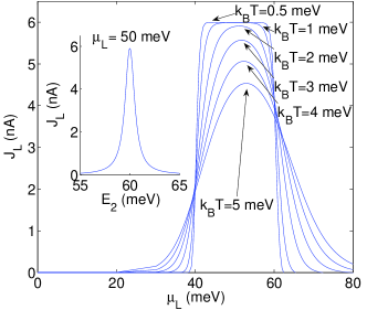
Figure 2: Currents as a function of $\mu_{L}$ and $E_{2}$ (subfigure). Other parameters from Table 1 (simplified system).

In Fig. 2 we show the current as a function of the left Fermi level $\mu_{L}$. There is no current until the left Fermi level comes within the vicinity of the ground-state of the first dot ($E_{1}=40$ meV). At this point electrons start to flow from the left lead into this state and further into the excited state of the second dot. If both states 1 and 4 are occupied, the Coulomb scattering via $U_{\mathrm{sc}}$ is possible. This process transfers one electron from level 1 to level 2 and a second electron from level 4 to level 3, which can subsequently reach the right lead via level 6. Thus Coulomb scattering establishes a transport path through the nanosystem. However, when the left Fermi level comes into the vicinity of the excited state of the first dot ($E_{2}=60$ meV) electrons will start to occupy this state. This causes a decrease in the current (see Fig. 2) as Pauli blocking hinders the scattering process addressed above. Likewise the temperature dependence essentially follows the probability

$$F=f_{L}(E_{1})f_{L}(E_{4})[1-f_{L}(E_{2})][1-f_{R}(E_{3})]$$ (13)

to find states $1$ and $4$ occupied while states $2$ and $3$ are empty. The relevance of level $E_{2}$ for the transport is further demonstrated in the subfigure of Fig. 2, showing that current only flows through the triple-dot structure if $E_{2}-E_{1}\approx E_{4}-E_{3}$, where the Coulomb scattering is energetically allowed.

This presence of current enhancement in a finite bias window $\Delta\mu_{L}$ matching the energy transfer $\Delta E$ by the scattering process is the characteristic signal of electron transport by Coulomb scattering. This Pauli-blocking of the scattering from level 4 to level 3 by occupation of the further level 2 does not appear for other inelastic scattering mechanisms such as phonon scattering.

IV Description by scattering

The description based on scattering given above becomes quantitative if the Coulomb scattering is the limiting process for transport through the device, i.e., if $U_{\mathrm{sc}}$ is significantly smaller than $\Omega_{14}$ and $\Omega_{36}$. For this reason, we have performed calculations for the increased values $\Omega_{14}=\Omega_{36}=1$ meV, see Fig. 3. The strong coupling between the states $3$ and $6$ yields a bonding and an anti-bonding state, with energies $20\mp 1$ meV. Therefore the resonance condition for Coulomb scattering is now satisfied at $E_{2}=59$ meV and $E_{2}=61$ meV (not shown) as displayed in the right subfigure of Fig. 3.

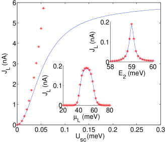
Figure 3: Current as a function of $U_{\mathrm{sc}}$ with $\Omega_{14}=\Omega_{36}=1$ meV and $E_{2}=59$ meV. The two subfigures show the current for $U_{\mathrm{sc}}=0.01$ meV as a function of $\mu_{L}$ and $E_{2}$, respectively. Other parameters from Table 1 (simplified system). The solid lines are calculated by the first-order von Neumann approach and the dots depict $J_{L}=eR_{\mathrm{tr}}$, where $R_{\mathrm{tr}}$ is the transition rate, Eq. (14), for the electron-electron scattering process.

Fermi’s golden rule provides us with the transition rate by Coulomb scattering into the anti-bonding state between 3 and 6:

$$\begin{split}R_{\mathrm{tr}}=&\frac{U_{\mathrm{sc}}^{2}}{2\hbar}\frac{\Gamma_{\mathrm{eff}}}{(E_{2}+E_{3}+\Omega_{36}-E_{1}-E_{4})^{2}+\Gamma_{\mathrm{eff}}^{2}/4}F\end{split}$$ (14)

Here we have replaced the energy-conserving $\delta$-function by a Lorentzian, representing life-time broadening due to the coupling to leads. $\Gamma_{\mathrm{eff}}=2\Gamma_{L}+\Gamma_{R}/2$ is the sum of broadenings for the individual states: $\Gamma_{L}$ for the levels 1 and 2, and $\Gamma_{R}/2$ for the anti-bonding combination of 3 and 6. Fig. 3 shows that Fermi’s golden rule provides a full quantitative description for small $U_{\mathrm{sc}}$. However, for larger values of $U_{\mathrm{sc}}$, this simple reasoning, based on single-particle states, fails. In particular, the width of the current peak becomes much broader than the simple life-time broadening $\Gamma_{\mathrm{eff}}$ (see subfigure of Fig. 2), which makes it easier to observe the effect in a real system with imprecise control over the level energies.

V Description by many-particle states

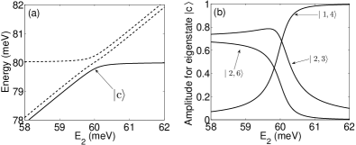
Figure 4: a) Energies of selected two-particle states as a function of $E_{2}$. b) Coefficients of state $|c\rangle$. Other parameters from Table 1 (simplified system).

Now we want to sketch, how this scattering-induced transport emerges within a basis of many-particle states, which takes into account the entire Coulomb interaction. For the parameters of Table 1 the anti-symmetrized two-particle product states $|1,4\rangle$, $|2,3\rangle$, and $|2,6\rangle$ all have the same sum of single-particle energies $E_{i}+E_{j}=80$ meV. They couple to each other due to the matrix elements $U_{\mathrm{sc}}$ and $\Omega_{36}$, resulting in the three many-particle states depicted in Fig. 4. For $E_{2}\approx 60$ meV, the three states are highly entangled and we focus in the following on one of these entangled states, denoted by $|c\rangle$. This state contributes to a circle of transitions between different many-particle states depicted in Fig. 5:

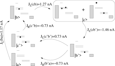
Figure 5: Diagrammatic representation of a circle of transport processes involving the many-particle states $|b\rangle$, $|c\rangle$, $|b^{\prime}\rangle$, $|a\rangle$, and $|c\rangle$. The two sets of double lines are the bonding and anti-bonding combinations of the states $1$, $4$ and $3$, $6$, respectively.

The state $|c\rangle$ can be reached by tunneling of an electron from the left lead into the state $|b\rangle$ (process from upper left to upper right). Here $|b\rangle$ is the binding one-particle state combining levels 1 and 4. By removing an electron towards the left lead (at a higher energy than before), the state $|c\rangle$ decays to the one-particle state $|b^{\prime}\rangle$, the binding state combining levels 3 and 6. Then the original state $|b\rangle$ is restored by one electron tunneling from the state $|b^{\prime}\rangle$ to the right lead and one electron tunneling into the state $|b\rangle$ from the left lead, which can happen in two different sequential orders. The key issue for the existence of this circle is the presence of the entangled state $|c\rangle$, which enables the transition between $|b\rangle$ and $|b^{\prime}\rangle$ via two single-electron tunneling processes. Therefore the current drops, if the product states $|1,4\rangle$ and $(|2,3\rangle+|2,6\rangle)/\sqrt{2}$ are detuned by varying $E_{2}$.

The currents $J_{L/R}(cb)$ in Fig. 5 denote the contribution of the transitions $b\leftrightarrow c$ between the corresponding many-particle states to the current from the left/right lead into the system, respectively, as given in Eq. (12). The magnitude of these currents corresponds to the transition rate between the states. Fig. 5 shows that the ingoing and outgoing rates partially balance for all states depicted. Nevertheless, there are plenty of further transitions, which make the full picture far more involved. In total this circle provides $J_{L}=1.71$ nA and $J_{R}=-1.46$ nA, which constitutes only a part of the total current $J_{L}=-J_{R}=5.9$ nA. The remaining part is carried by similar circles involving the other many-particle states as well as more complicated transitions which cannot be separated into circles that easily.

Finally, note that the electrons enter the structure with $E\approx E_{1}$ from the left contact and leave the structure with $E\approx E_{5}$ to the right contact as well as with $E\approx E_{2}$ to the left contact. Thus there is no single transmission channel at a given energy as typical for the frequently used transmission models.

VI Results for the full system

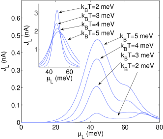
Figure 6: Current as a function of $\mu_{L}$ for different temperatures. Other parameters from Table 1. In the subfigure the single-particle energies $E_{1}=43$ meV, $E_{2}=63$ meV, $E_{3}=20$ meV, $E_{4}=40$ meV, $E_{5}=-4$ meV, and $E_{6}=16$ meV are used.

In Fig. 6 we present results for the full system, i.e., using all parameters given in Table 1. Like in Fig. 2 we observe a current signal in a finite region of $\mu_{L}$, which is a key feature of the current induced by electron-electron scattering (the current is below 0.006 nA if $U_{\mathrm{sc}}=0$ is used). However, contrary to the simplified system in Fig. 2, the peak current increases with temperature for the full system and is much weaker. This is due to the presence of an electron in state $5$ which breaks the alignment between the levels 3 and 6 by Coulomb repulsion. With increasing temperature, the probability for state 5 to be empty increases and so does the current. In the subfigure of Fig. 6 we show results for a case where the single-particle energies have been modified to compensate for charging effects, which provides results similar to Fig. 2. In both cases we observe enhanced current in (multiple) finite bias windows $\Delta\mu_{L}$ matching the energy transfer $\Delta E$, which are however smeared out by temperature. This shows that the essential features of transport by electron-electron scattering are robust with respect to other electron-electron interaction mechanisms.

VII Conclusion

We have shown that Coulomb scattering provides a current channel for transport through a triple-dot system. The mechanism holds for general nanosystems exhibiting two pairs of states with a similar level spacing $\Delta E$. An example is the conduction through a macro molecule, where an appropriate chemical group appears twice. A typical signature is a current signal for a finite bias window, matching the energy transfer $\Delta E$. If the Coulomb scattering is the slowest transfer process involved, a simple description based on Fermi’s golden rule is valid. Otherwise a systematic implementation is possible within a basis of many-particle states, which reflects the total Coulomb interaction for the nanosystem.