Coil-Stretch Transition and the Break Down
of Continuum Models

Abstract

The breakdown of finite element (FEM) computations for the flow of an Oldroyd-B fluid around a cylinder confined between parallel plates, at Weissenberg numbers $W\!i=\mathcal{O}(1)$, is shown to arise due to a coil-stretch transition experienced by polymer molecules traveling along the centerline in the wake of the cylinder. With increasing $W\!i$, the coil-stretch transition leads to an unbounded growth in the stress maximum in the cylinder wake. Finite element computations for a FENE-P fluid reveal that, although polymer molecules undergo a coil-stretch transition in the cylinder wake, the mean extension of the molecules saturates to a value close to the fully extended length, leading to bounded stresses with increasing $W\!i$. The existence of a coil-stretch transition has been deduced by examining the behavior of ultra-dilute Oldroyd-B and FENE-P fluids. In this case, the solution along the centerline in the cylinder wake can be obtained exactly since the velocity field is uncoupled from the stress and conformation tensor fields. Estimation of the number of finite elements required to achieve convergence reveals the in-feasibility of obtaining solutions for the Oldroyd-B model for $W\!i>1$.

I Introduction

The behavior of polymeric liquids in complex flows is intimately linked to the distribution of molecular conformations in the flow field. Macroscopic field variables such as the stress and velocity are strongly coupled to microscopic quantities such as the stretch and orientation of polymer molecules, and they influence and determine the magnitude of each other. Recent advances in computational rheology have led to the development of micro-macro methods that are capable of resolving information at various length and time scales. However, because of computational cost, most numerical simulations are still based on the purely macroscopic approach of continuum mechanics, where the conservation laws of mass and momentum are solved with a constitutive equation that relates the stress to the deformation history, without explicitly accounting for the microstructure Keunings [2000]. The simplest constitutive equations capable of capturing some qualitative aspects of the viscoelastic behavior of polymer solutions and melts are the Oldroyd-B and upper convected Maxwell models, respectively. These models have been widely used in the investigation of complex flows since the early days of computational rheology Owens and Phillips [2002].

In spite of the apparent simplicity of the macroscopic equations, obtaining solutions at industrially relevant values of the Weissenberg number $W\!i$ has proven to be extremely difficult in a range of flow geometries. Careful numerical studies over the past few decades suggest that the principal source of computational difficulties is the emergence of large stresses and stress gradients within narrow regions of the flow domain. Significant efforts have been made to develop grid-based numerical techniques for resolving these stresses and their gradients. In spite of considerable progress, numerical solutions still breakdown at disappointingly low values of $W\!i\sim\mathcal{O}(1)$, and it is still not clear whether this is because solutions do not exist at higher values of $W\!i$, or whether it is simply due to the inadequacy of current numerical techniques Keunings [2000]. Very recently, Renardy [2006] has shown analytically that in the special case of steady flows with an interior stagnation point, the mathematical structure of the upper convected Maxwell and Oldroyd-B models can be expected to lead to singularities in the viscoelastic stresses and their gradients with increasing $W\!i$.

Nearly two decades ago, Rallison and Hinch [1988] argued in a seminal paper that in the case of the Oldroyd-B model, the inability to compute macroscopic flows at high Weissenberg numbers (the so called high Weissenberg number problem, or HWNP), has a physical origin in a microscopic phenomenon. The Oldroyd-B model predicts an unbounded extensional viscosity in homogenous extensional flows at a critical value of $W\!i$. The Oldroyd-B constitutive equation can be derived from kinetic theory by representing polymer molecules by Hookean dumbbells. The unphysical behavior in extensional flows is due to the infinite extensibility of the Hookean spring used in the model. By considering the simple example of a stagnation point flow of an Oldroyd-B fluid, Rallison and Hinch showed that when the strain rate is supercritical, infinite stresses can occur in the interior of a steady flow, brought about by the unbounded stretching of polymer molecules. Based on their analysis, they suggested the use of a constitutive equation that is derived from a microscopic model with a nonlinear spring force law (which would impose a finite limit on a polymers extension), as an obvious remedy for the HWNP.

Chilcott and Rallison [1988] examined the benchmark complex flow problems of unbounded flow around a cylinder and a sphere, using a dumbbell model with finite extensibility, as a means of demonstrating the validity of this analysis. In order to understand the coupling between the polymer extension by flow, the stresses developed in the fluid, and the resultant flow field, they deliberately used the conformation tensor as the fundamental variable instead of the stress. The conformation tensor gives information on the distribution of polymer conformations within the flow field in an averaged sense. The use by Chilcott and Rallison of kinetic theory to develop their model enabled the derivation of a simple expression relating the conformation tensor to the polymer contribution to the stress. By solving the equation for the conformation tensor along with the mass and momentum conservation laws, Chilcott and Rallison showed that even though there existed highly extended material close to the boundary and in the wake of the obstacle, there no longer was an upper limit to $W\!i$ in the range of values that was examined in their computations. Since the degree of molecular extension is directly related to the magnitude of stress, the Chilcott and Rallison procedure established a clear connection between high stresses and stress gradients in the flow domain with the configurational and spatial distribution of polymer conformations. Indeed, when simulations were carried out with the polymer length set to infinity rather than a finite value, the downstream structure was no longer resolvable, and the mean stretch of the polymers in the flow direction continued to grow with increasing $W\!i$ until the solution failed.

In spite of this compelling demonstration of the physical origin of the HWNP, the upper convected Maxwell and Oldroyd-B models have continued to be used extensively in computational rheology. The reason for this might perhaps be attributed to the fact that even though stresses may be large, they are still bounded, and so far, there has been no conclusive demonstration that bounded solutions for the viscoelastic stress do not exist in complex flows at high values of $W\!i$. On the contrary, by considering the steady flow of upper convected Maxwell and Oldroyd-B fluids around a cylinder confined between two parallel plates (a schematic of the flow geometry is displayed in Fig. 1), Wapperom and Renardy [2005] have presented strong numerical evidence that suggests that solutions do exist for $W\!i>1$, and that current numerical techniques are not able to resolve them.

\psfrag{Z}{\large${\bf v}_{\bf x}={\bf f(y)}$}\psfrag{A}{\large${\bf v}_{\bf y}={\bf 0}$}\psfrag{B}{\large${\bf v}\cdot{\mbox{\boldmath$\nabla$}}{{\bf M}}={\bf 0}$}\psfrag{F}{\large${\bf v}_{\bf x}={\bf f(y)}$}\psfrag{G}{\large${\bf v}_{\bf y}={\bf 0}$}\psfrag{M}{\large${\bf v}={\bf 0}$}\psfrag{D}{\large${\bf t}{\bf n}:{(\bm{\tau}_{\text{s}}+\bm{\sigma})}=0$}\psfrag{E}{\large${\bf v}_{\bf y}={\bf 0}$}\includegraphics*{Fig1.eps}

Figure 1: Flow domain and boundary conditions for the flow around a cylinder confined between parallel plates.

The particular benchmark problem of flow around a cylinder between parallel plates was chosen by these authors since even though the geometry has no singularities, the maximum values of $W\!i$ for which converged solutions exist are amongst the smallest of all benchmark flows Fan et al. [1999]; Sun et al. [1999]; Alves et al. [2001]; Caola et al. [2001]; Oscar et al. [2006]. The presence of upstream and downstream stagnation points leads to the development of steep stress boundary layers near the cylinder and in the wake of the cylinder, making the flow a stringent test of any numerical technique. Rather than solving the coupled problem simultaneously for the velocity and conformation tensor fields, for which the existence of solutions at high $W\!i$ is unknown, Wapperom and Renardy assumed a Newtonian-like velocity field and solved only for the conformation tensor field. The chosen velocity field has an analytical representation, is very similar to the Newtonian velocity field in the same geometry (and the velocity field for an Oldroyd-B fluid at $W\!i\sim\mathcal{O}(1)$), and satisfies all the key requirements for the velocity field near the cylinder. The advantage of this approach is that the existence of a solution for an upper convected Maxwell model in such a velocity field, at all values of $W\!i$ is guaranteed Renardy [2000], and hence failure of a numerical scheme can be attributed purely to numerics. By developing a Lagrangian technique which involves integrating the conformation tensor equation along streamlines using a predictor-corrector method, the authors were able to compute stresses up to arbitrarily large values of $W\!i$ (as high as 1024), and as a result, establish conclusively the existence of narrow regions with very high stresses near the cylinder, and in its wake. Further, they show that although the velocity field is known, one of the currently used numerical techniques, the backward-tracking Lagrangian technique, is unable to resolve the extremely thin stress boundary layers even for relatively low values of $W\!i$. Since the fully coupled problem and the fixed flow kinematics problem share the same basic dilemma of computing the stress field, Wapperom and Renardy argue that solutions also probably exist for $W\!i>1$ for the steady flow of Oldroyd-B and upper convected Maxwell fluids around a cylinder confined between parallel plates, but current numerical techniques are not able to resolve them.

The use of the conformation tensor as the fundamental quantity rather than the stress has become common in computational rheology, and the challenge of developing numerical methods capable of resolving steep stresses and stress gradients has been transformed to one of developing techniques capable of resolving rapidly varying conformation tensor fields. In an important recent breakthrough, Fattal and Kupferman [2004] have shown that by changing the fundamental variable to the matrix logarithm of the conformation tensor, stable numerical solutions can be obtained at values of $W\!i$ significantly greater than ever obtained before. The success of their variable transformation protocol is predicated on their identification of the source of the HWNP as the inability of methods based on polynomial basis functions (such as finite element methods), to adequately represent the exponential profiles that emerge in conformational tensor fields in the vicinity of stagnation points and in regions of high deformation rate.

Hulsen et al. [2005] have recently carried out a stringent test of the log conformation representation by examining the flow of Oldroyd-B and Giesekus fluids around a cylinder confined between parallel plates. (It is worth noting that unlike the Oldroyd-B models prediction of unbounded extensional viscosity at a finite extension rate, the extensional viscosity predicted by the Giesekus model is always finite Bird et al. [1987a]). For both the fluids, Hulsen et al. [2005] find that with the log conformation formulation, the solution remains numerically stable for values of $W\!i$ considerably greater than those obtained previously with standard finite element (FEM) implementations. On the other hand, the two fluids differ significantly from each other with regard to the behavior of the convergence of solutions with mesh refinement. The lack of convergence with mesh refinement is usually seen most dramatically in the failure of different meshes to accurately predict the maximum that occurs in the normal polymeric stress component ${\sigma}_{xx}$ on the centerline in the wake of the cylinder. In the case of the Giesekus model, even at values of Weissenberg number as high as $W\!i=100$, mesh convergence is achieved in large parts of the flow domain, with the exception of localized regions near the stress maximum in the wake where convergence is not realized. For the Oldroyd-B model, however, the log conformation formulation fails to achieve mesh convergence in the entire wake region at roughly the same value ($W\!i\gtrsim 0.6$) as in previous studies. Further, the solution becomes unsteady at some greater value of $W\!i$ (depending on the mesh), finally breaking down at even higher $W\!i$. Hulsen et al. [2005] speculate that this failure is probably due to the infinite extensibility of the Hookean dumbbell model that underlies the Oldroyd-B model, and call for further investigations to see if this might lead to the non-existence of solutions beyond some value of $W\!i$. Thus, after many years of attempting to resolve the HWNP by purely numerical means, it’s origin still remains a mystery.

In this paper, we conclusively establish the connection between the HWNP and the unphysical behavior of the Oldroyd-B model, in the benchmark problem of the steady flow around a cylinder confined between parallel plates. We show that when $W\!i\approx 1$, polymer molecules flowing along the centerline in the wake of the cylinder undergo a coil-stretch transition, and that the location of the transition coincides with the maximum in the normal stress component ${\sigma}_{xx}$ on the centerline. With increasing $W\!i$, the molecules stretch without bound, and this is accompanied by a normal stress that increases without bound. (For an UCM fluid, Alves et al. [2001] have previously speculated that ${\sigma}_{xx}$ may develop a singularity at the position where it reaches a maximum value, based on the asymptotic behavior of highly accurate numerical results obtained by them using a finite volume method. However, they were unable to attribute a precise reason for the occurrence of a singularity). Computations carried out here for a FENE-P fluid reveal that in this case also, polymer molecules undergo a coil-stretch transition which is located at the stress maximum. However, with increasing $W\!i$, the mean extension of the molecules saturates to a value close to their fully extended length, enabling computations beyond the critical Weissenberg number.

These dilute solution results have been obtained by drawing on insights gained from the solution of an ultra-dilute model, in which the velocity field is decoupled from the conformation tensor (and stress) field. This procedure is similar to the earlier work by Wapperom and Renardy [2005] described above. However, rather than using an ad hoc velocity field, we have solved for the Newtonian velocity field using a full-fledged FEM simulation. Even for the ultra-dilute model, with a known velocity field, the solution of the equation for the conformation tensor (which is denoted here by ${\bf M}$) for the Oldroyd-B model is found to breakdown for $W\!i\sim\mathcal{O}(1)$, when a standard FEM method is used. However, an exact (numerical) solution for ${\bf M}$, valid for arbitrary large values of $W\!i$, is obtained along the centerline using two different techniques. In the first method, we exploit the fact that the equation for ${\bf M}$ in the Oldroyd-B and FENE-P models reduces at steady state to a system of ordinary differential equations (ODEs) along the centerline. In the second method, trajectories of the end-to-end vectors of an ensemble of dumbbells, flowing down the centerline in the wake of the cylinder, are calculated by carrying out Brownian dynamics simulations using the known velocity field. Averages carried out over the ensemble of trajectories lead to macroscopic predictions that are identical to the exact (numerical) results obtained by solving the macroscopic model ODEs discussed above, for arbitrary values of $W\!i$. Comparison of the FEM results with the exact numerical results enables a careful examination of the reasons for the breakdown of the finite element method. In particular, the occurrence of a coil-stretch transition at the location of the stress maximum in the wake is clearly demonstrated, and an estimation of the number of elements in the FEM method required to achieve convergence with increasing $W\!i$ reveals the in-feasibility of obtaining solutions for $W\!i>1$.

The plan of this paper is as follows. In section II, we summarize the governing equations, boundary conditions and computational method for the flow of dilute Oldroyd-B and FENE-P fluids around a cylinder confined between parallel plates. We also elaborate on the connection between the macroscopic models, and the Kinetic theory models from which they are derived. In section III, we describe the means by which exact solutions to the ultra-dilute models may be obtained, and examine the nature of the maximum in the $\text{M}_{xx}$ component of the conformation tensor. The results of FEM computations and the exact numerical methods are first discussed for ultra-dilute solutions in section IV, followed by a discussion of the predictions of FEM computations for the dilute model. Section V summarizes the main conclusions of this work.

II Dilute Solutions

II.1 Basic equations

As displayed in Fig. 1, the cylinder axis is in the $z$-direction perpendicular to the plane of flow. With the assumption of a plane of symmetry along the centreline ($y=0$), computations are only carried out in half the domain. The cylinder, with radius $a$, is assumed to be placed exactly midway between the plates, which are separated from each other by a distance $2H$. In common with other benchmark flow around a confined cylinder simulations, we set the blockage ratio $H/a=2$.

We normalize all macroscopic length scales with respect to $a$, velocities with respect to the mean inflow velocity far upstream ${\bigl{\langle}}v{\bigr{\rangle}}$, macroscopic time scales with respect to $a/{\bigl{\langle}}v{\bigr{\rangle}}$, and stresses and pressure with respect to $\eta\,{{\bigl{\langle}}v{\bigr{\rangle}}}/a$, where $\eta=\eta_{\text{s}}+\eta_{\text{p,0}}$ is the sum of the Newtonian solvent viscosity $\eta_{\text{s}}$ and the zero-shear rate polymer contribution to viscosity $\eta_{\text{p,0}}$. Microscopic length and time scales are discussed subsequently. The two dimensionless numbers of relevance here are the Weissenberg number $W\!i=\lambda\,{{\bigl{\langle}}v{\bigr{\rangle}}}/a$, in which $\lambda$ is a relaxation time, and the Reynolds number $Re=\rho\,a\,{{\bigl{\langle}}v{\bigr{\rangle}}}/\eta$, where $\rho$ is the fluid density.

The complete set of non-dimensional governing equations for a dilute polymer solution, described by the Oldroyd-B or FENE-P models, is

$${\bf\nabla}\cdot{\bf v} =0$$ (Mass balance) (1)

$$Re\,{\bf v}\cdot{\bf\nabla}{\bf v}-{\bf\nabla}p-{\bf\nabla}\cdot\bm{\tau}_{\text{s}}-{\bf\nabla}\cdot\bm{\sigma} ={\bf 0}$$ (Momentum balance) (2)

$$\frac{\partial{\bf M}}{\partial t}+{\bf v}\cdot\nabla{\bf M}-\bm{\kappa}\cdot{\bf M}-{\bf M}\cdot\bm{\kappa}^{T} =-\frac{1}{W\!i}\left\{f(\mathrm{tr}\,{\bf M})\,{\bf M}-{\bf I}\right\}$$ (Conformation tensor) (3)

$$\bm{\tau}_{\text{s}} =2\,\beta\,{\bf D}$$ (Solvent stress) (4)

$$\bm{\sigma} =\frac{(1-\beta)}{W\!i}\left\{f(\mathrm{tr}\,{\bf M})\,{\bf M}-{\bf I}\right\}$$ (Polymer stress) (5)

In these equations, $\bm{\kappa}=(\nabla{\bf v})^{T}$ is the transpose of the velocity gradient, ${\bf D}=\frac{1}{2}\left(\bm{\kappa}^{T}+\bm{\kappa}\right)$ is the rate of deformation tensor, and the parameter $\beta=(\eta_{\text{s}}/\eta)$ is the viscosity ratio. Here, we use $\beta=0.59$, and set $Re=0$, which are the values used in benchmarks for the Oldroyd-B model. The form of the function $f(\mathrm{tr}\,{\bf M})$ depends on the microscopic model used to derive the equation for the evolution of the conformation tensor, and is consequently different in the Oldroyd-B and FENE-P models, as elaborated below.

II.1.1 Oldroyd-B model

As mentioned earlier, the Oldroyd-B constitutive equation can be derived from Kinetic theory, with the polymer molecule represented by a Hookean dumbbell model consisting of two beads connected together by a spring Bird et al. [1987b]. The spring obeys a linear spring force law ${\bf F}^{\text{(s)}}=H{\bf Q}$, where $H$ is the spring constant, and ${\bf Q}$ is the connector vector between the beads. In this model, the conformation tensor ${\bf M}$ is defined by the expression,

$${\bf M}=\frac{1}{({\bigl{\langle}}Q^{2}{\bigr{\rangle}}_{\text{eq}}/3)}\,{\bigl{\langle}}{\bf Q}{\bf Q}{\bigr{\rangle}}$$ (6)

where, ${\bigl{\langle}}(.){\bigr{\rangle}}$ denotes an ensemble average, and $\sqrt{{\bigl{\langle}}Q^{2}{\bigr{\rangle}}_{\text{eq}}}$ is the root mean square end-to-end vector at equilibrium. Note that, $\sqrt{{\bigl{\langle}}Q^{2}{\bigr{\rangle}}_{\text{eq}}/3}=\sqrt{k_{\text{B}}T/H}$ (with $k_{\text{B}}$ being the Boltzmanns constant and $T$ the temperature), is the microscopic length scale. The connection between the microscopic and macroscopic models is established by deriving an evolution equation for the conformation tensor, and by relating the macroscopic polymeric stress to the conformation tensor. The expression of the conformation tensor is given by eqn (3) above, where in this case, the function $f$ is identically equal to unity, i.e. $f(\mathrm{tr}\,{\bf M})=1$. The polymer contribution to the stress is given by Kramers expression Bird et al. [1987b],

$$\bm{\sigma}=n\,k_{\text{B}}T\,\left\{{\bf M}-{\bf I}\right\}$$ (7)

where, $n$ is the number density of polymer molecules in solution. With the relaxation time $\lambda$, and the zero-shear rate polymer contribution to the viscosity $\eta_{\text{p,0}}$, of the Oldroyd-B model related to microscopic model parameters by,

$$\lambda=\frac{\zeta}{4H}\,;\quad\eta_{\text{p,0}}=nk_{\text{B}}T\,\lambda$$ (8)

where, $\zeta$ is the bead friction coefficient, it is straightforward to see that the non-dimensionalization scheme used here leads to equation (5) for $\bm{\sigma}$.

II.1.2 FENE-P model

The FENE-P model corrects the failing of the Hookean dumbbell model with its infinite extensibility, by using a spring force law that ensures that the magnitude of the end-to-end vector remains (on an average) below the fully extensible length of the spring $Q_{0}$,

$${\bf F}^{\text{(s)}}=\frac{H}{\left(1-{{\bigl{\langle}}Q^{2}{\bigr{\rangle}}}/{Q_{0}^{2}}\right)}\,{\bf Q}$$ (9)

For the FENE-P model, the conformation tensor is also defined by eqn (6), but with the mean square end-to-end vector at equilibrium ${{\bigl{\langle}}Q^{2}{\bigr{\rangle}}_{\text{eq}}}$ given by,

$${\bigl{\langle}}Q^{2}{\bigr{\rangle}}_{\text{eq}}=\frac{3\,Q_{0}^{2}\,(k_{\text{B}}T/H)}{Q_{0}^{2}+3\,(k_{\text{B}}T/H)}$$ (10)

Defining the finite extensibility parameter $b$ by,

$$b=\frac{Q_{0}^{2}}{{\bigl{\langle}}Q^{2}{\bigr{\rangle}}_{\text{eq}}}$$ (11)

the function $f(\mathrm{tr}\,{\bf M})$ for the FENE-P model in the conformation tensor evolution equation (3) can be shown to be given by Pasquali and Scriven [2002],

$$f(\mathrm{tr}\,{\bf M})=\frac{b-1}{b-\mathrm{tr}\,{\bf M}/3}$$ (12)

Note that the definition of $b$ used in eqn (11) is different from the definition of the finite extensibility parameter given in Bird et al. [1987b], which is widely used in the literature. In the Bird et al.  definition, the microscopic length scale used to non-dimensionalize $Q_{0}$ is the Hookean dumbbell length scale $\sqrt{k_{\text{B}}T/H}$. The polymeric stress for a FENE-P fluid is given by,

$$\bm{\sigma}=n\,k_{\text{B}}T\,\left\{f(\mathrm{tr}\,{\bf M})\,{\bf M}-{\bf I}\right\}$$ (13)

With the relaxation time $\lambda$, and the zero-shear rate polymer contribution to the viscosity $\eta_{\text{p,0}}$ related to microscopic model parameters by,

$$\lambda=\left(\frac{b-1}{b}\right)\frac{\zeta}{4H}\,;\quad\eta_{\text{p,0}}=nk_{\text{B}}T\,\lambda$$ (14)

non-dimensionalization of eqn (13) leads to eqn (5).

Table 1: Meshes used in the finite element simulations for computing viscoelastic flow around a cylinder.

Mesh	M1	M2	M3	M4	M5
Number of Elements	2311	5040	8512	16425	31500

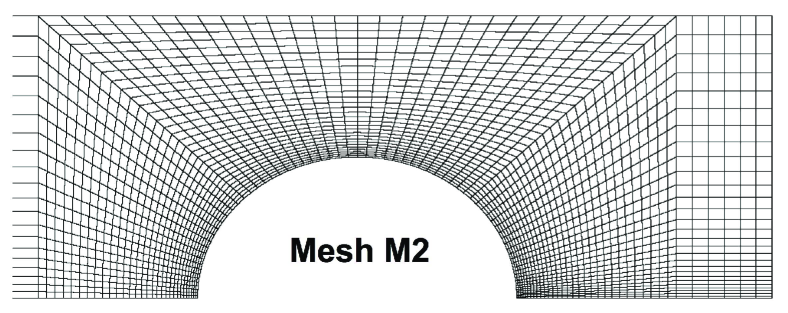
Figure 2: Mesh M2 used in the finite element simulations.

II.2 Boundary conditions and computational method

The set of governing equations (1)-(5) are solved with the boundary conditions shown in Fig. 1. The location of the inflow and outflow boundaries coincides with that chosen by Sun et al. [1999], who showed that the flow is insensitive to further displacement of the open boundaries in the range of Weissenberg numbers examined. A no-slip boundary condition is imposed on the cylinder surface and the channel walls. Fully developed flow is assumed at both inflow and outflow boundaries, with the velocity prescribed at both boundaries. Here, ${\bigl{\langle}}v{\bigr{\rangle}}=1$ for the prescribed velocity field. The boundary conditions on the conformation tensor are imposed only at the inflow boundary. At the symmetry line, ${\bf t}{\bf n}:{(\bm{\tau}_{\text{s}}+\bm{\sigma})}=0$ and $v_{y}=0$ is imposed, where, ${\bf t}$ and ${\bf n}$ are the unit vectors tangential and normal to the symmetry line, respectively.

The governing equations are discretized by using the DEVSS-TG/SUPG mixed finite element method Pasquali and Scriven [2002]. The DEVSS-TG formulation involves the introduction of an additional variable, the velocity gradient $\bm{\kappa}$. Continuous biquadratic basis functions are used to represent velocity, linear discontinuous basis functions to represent pressure and continuous bilinear basis functions are used for the interpolated velocity gradient and conformation tensor. The DEVSS-TG/SUPG spatial discretization results in a large set of coupled non-linear algebraic equations, which are solved by Newton’s method with analytical Jacobian and first order arc-length continuation in $W\!i$ Pasquali and Scriven [2002]. Five different meshes are used for the FEM calculations. Details of the different meshes used in this work are given in Table 1, and the mesh M2 is displayed in Fig. 2. The important distinction among the five meshes is the density of elements on the cylinder surface and in the wake of the cylinder.

III Ultra-Dilute Solutions

The phrase “ultra-dilute” is used to describe a situation where, even though polymer molecules are present, they have a negligible effect on the velocity field. As demonstrated in the earlier work by Wapperom and Renardy [2005] , the solution of the ultra-dilute problem provides important insights into the structure of the solution to the dilute problem, where the polymer stress and velocity fields are fully coupled. As will be clear from the results and discussion presented subsequently, the solution of the ultra-dilute case lies at the heart of the analysis carried out in this work.

Since the velocity field for an ultra-dilute solution is determined completely by the solvent stress, it is identical to the velocity field for a Newtonian fluid. The ultra-dilute conformation tensor and velocity fields are simply obtained by solving the governing equations with the parameter $\beta$ set equal to unity. As can be seen from eqn (5), this implies $\bm{\sigma}=0$, leading to eqns (1) and (2) being identical to the mass and momentum balances for a Newtonian fluid. The same FEM formulation described above for the solution of the dilute case, can consequently, also be used to obtain the ultra-dilute conformation tensor and Newtonian velocity fields when $\beta=1$.

The conformation tensor field, for an ultra-dilute solution, corresponds to the average configurations of polymer molecules in a pre-determined velocity field. Note that the choice of value for $W\!i$ has no influence on the velocity field (which is determined once and for all for the specified geometry), but can significantly effect the conformation tensor field, as will be seen subsequently.

Clearly, the polymer contribution to the stress tensor cannot be obtained from a solution of the macroscopic equations, where it is assumed to be zero. In this case, we resort to reporting the dimensionless stress predicted by the microscopic models, $\bm{\sigma}^{*}=\bm{\sigma}/n\,k_{\text{B}}T=(\lambda/\eta_{\text{p,0}})\,\bm{\sigma}$, given by eqns (7) and (13), in the Oldroyd-B and FENE-P models, respectively. This is similar to the evaluation of the polymer contribution to the stress in a homogenous simple shear or extensional flow, where the velocity field is prescribed a priori.

As mentioned earlier, the FEM formulation used here fails to give mesh-converged results for the conformation tensor field for an ultra-dilute solution beyond a threshold value of the Weissenberg number. The reasons for this failure are analyzed subsequently. Crucial for this analysis, however, is the possibility of obtaining an exact (numerical) solution to the conformation tensor equation along the centerline in the wake of the cylinder. Two means of obtaining such a solution are discussed below.

III.1 Exact (numerical) solution along the centerline in the cylinder wake

III.1.1 System of ODEs

By the requirements of symmetry along the centerline, the velocity field must have the form, $v_{x}=g(x)$, $v_{y}=0$, and the components of the velocity gradient tensor must satisfy, $\kappa_{xy}=\kappa_{yx}=0$. Incompressibility requires $\kappa_{xx}=-\kappa_{yy}$. The flow along the centerline is consequently planar extensional in character.

Substituting these results into the evolution equation for the conformation tensor (eqn (3)) leads, at steady state, to a system of ODEs in the independent variable $x$, for the components of the conformation tensor ${\bf M}$. In the case of the Oldroyd-B model, the equations for each of the components are decoupled from each other. For the purposes of analysis in the present work, we are only interested in the equation for the $\text{M}_{xx}$ component, which can be shown to be,

$$\frac{d\text{M}_{xx}}{dx}=-\frac{(1-2\lambda\kappa_{xx}(x))}{\lambda v_{x}(x)}\,\text{M}_{xx}+\frac{1}{\lambda v_{x}(x)}$$ (15)

Since the velocity field is known a priori, equation (15) is a first order liner ODE for $\text{M}_{xx}$ that can be solved straight-forwardly once a boundary condition is prescribed. We can expect that at the downstream stagnation point at $x=1$, the Hookean dumbbells that represent the polymer molecules are in their equilibrium configurations, and consequently $\text{M}_{xx}=1$. However, as can be seen from the form of eqn (15), we cannot use this boundary condition since $v_{x}=0$ at the stagnation point. We can overcome this difficulty by exploiting the fact that we can guess the form of the velocity field asymptotically close to the stagnation point. For an unbounded flow of a Newtonian fluid near a stagnation point on the surface of a two-dimensional body, the assumption of a quadratic velocity field, asymptotically close to the stagnation point, is exactly valid for Stokes flow, and is consistent with the accepted numerical solution for Hiemenz flow Pozrikidis [1997]. The approximate Newtonian velocity field postulated by Wapperom and Renardy [2005] for the flow around a confined cylinder is also of the form $v_{x}=k\,(x-1)^{2}$ (see also Renardy [2000]), with $k=4$, in the limit as $x\to 1$ (from above). We find that the assumption of a quadratic velocity field, with a value of $k=4.178$, leads to an excellent fit of the Newtonian velocity field close to the downstream stagnation point obtained by the FEM solution. For a quadratic velocity field, eqn (15) admits an analytical solution for $\text{M}_{xx}$,

$$\text{M}_{xx}=1+2\alpha\,(x-1)+3\alpha^{2}\,(x-1)^{2}+3\alpha^{3}\,(x-1)^{3}+1.5\alpha^{4}\,(x-1)^{4}$$ (16)

where, $\alpha=2k\lambda$. As a result, we use the analytical value of $\text{M}_{xx}$ at $x=1.01$ as the boundary condition to integrate eqn (15), with a Runge-Kutta 4th order method. The functions $v_{x}(x)$ and $\kappa_{xx}(x)$ are obtained by interpolation from the Newtonian FEM solution, at each of the values of $x$ where they are required for the purpose of integration.

For the FENE-P model, the diagonal components are not decoupled from each other, and consequently, evaluation of the $\text{M}_{xx}$ component requires a solution of a system of ODEs for all the diagonal components, as can be seen from the equations below,

$$\frac{d\text{M}_{xx}}{dx} =-\frac{1}{\lambda v_{x}(x)}\,\left\{\frac{b-1}{b-\mathrm{tr}\,{\bf M}/3}-2\lambda\kappa_{xx}(x)\right\}\,\text{M}_{xx}+\frac{1}{\lambda v_{x}(x)}$$ (17)

$$\frac{d\text{M}_{yy}}{dx} =-\frac{1}{\lambda v_{x}(x)}\,\left\{\frac{b-1}{b-\mathrm{tr}\,{\bf M}/3}-2\lambda\kappa_{yy}(x)\right\}\,\text{M}_{xx}+\frac{1}{\lambda v_{x}(x)}$$

$$\frac{d\text{M}_{zz}}{dx} =-\frac{1}{\lambda v_{x}(x)}\,\left\{\frac{b-1}{b-\mathrm{tr}\,{\bf M}/3}\right\}\,\text{M}_{zz}+\frac{1}{\lambda v_{x}(x)}$$

It is difficult to solve these equations analytically even with the assumption of a quadratic velocity field close to the stagnation point. Since $\kappa_{xx}(x)\ll 1$ at $x=1.01$, we use the equilibrium initial conditions, $\text{M}_{xx}=1$, $\text{M}_{yy}=1$, and $\text{M}_{zz}=1$, as the boundary conditions, though these values are strictly correct only at the stagnation point $x=1$. It turns out, however, that the conformational tensor fields along the centerline, downstream of the stagnation point, are insensitive to a variation by a few percent, in the boundary values chosen for the diagonal components of ${\bf M}$ close to the stagnation point. (For instance, identical results are obtained if the boundary conditions for the Oldroyd-B model at $x=1.01$, are used instead).

III.1.2 Brownian dynamics simulations

An alternative means of obtaining an exact solution along the centerline in the cylinder wake is to exploit the connection between the macroscopic and microscopic models. If we imagine an ensemble of dumbbells at any position $x$ on the centerline, subject to the local velocity gradient, we expect that at steady state, the ensemble average ${\bigl{\langle}}{\bf Q}^{\dagger}{\bf Q}^{\dagger}{\bigr{\rangle}}={\bf M}$, where, ${\bf Q}^{\dagger}={\bf Q}/\sqrt{({\bigl{\langle}}Q^{2}{\bigr{\rangle}}_{\text{eq}}/3)}$. We could also imagine a packet of fluid with an ensemble of dumbbells, starting close to the stagnation point and traveling down the centerline with velocity $v_{x}(x)$, experiencing the local velocity gradient at each position $x$. In this case, the variation with time of ${\bigl{\langle}}{\bf Q}^{\dagger}{\bf Q}^{\dagger}{\bigr{\rangle}}$ would be equivalent to the variation of ${\bf M}$ with $x$ in the macroscopic models. The ensemble average ${\bigl{\langle}}{\bf Q}^{\dagger}{\bf Q}^{\dagger}{\bigr{\rangle}}$ can be obtained by integrating the stochastic differential equation (SDE),

$$d{\bf Q}^{\dagger}=\{\bm{\kappa}(t)\cdot{\bf Q}^{\dagger}-\frac{1}{2W\!i}\,f\left({\bigl{\langle}}{Q^{\dagger}}^{2}{\bigr{\rangle}}\right){\bf Q}^{\dagger}\}\,dt+\frac{1}{\sqrt{W\!i}}\,d{\bf W}^{\dagger}$$ (18)

which governs the stochastic dynamics of Hookean or FENE-P dumbbells subject to the time varying velocity gradient $\bm{\kappa}(t)$ Öttinger [1996]. Here, ${\bf W}^{\dagger}$ is a non-dimensional Wiener process, and

$$f\left({\bigl{\langle}}{Q^{\dagger}}^{2}{\bigr{\rangle}}\right)=\begin{cases}1&\text{for Hookean dumbbells},\\ ({b-1})/({b-{\bigl{\langle}}{Q^{\dagger}}^{2}{\bigr{\rangle}}/3})&\text{for FENE-P dumbbells}\end{cases}$$ (19)

is the same function for the FENE-P model as in eqn (12), with ${\bigl{\langle}}{Q^{\dagger}}^{2}{\bigr{\rangle}}$ taking the place of $\mathrm{tr}\,{\bf M}$.

The only remaining issue is to obtain $\kappa_{xx}(t)$ for a packet of fluid traveling down the centerline in the wake of the cylinder. This can be done in a straightforward way since we know $v_{x}(x)$ and $\kappa_{xx}(x)$ for a Newtonian fluid. Since $dx/dt=v_{x}(x)$, the integral,

$$t=\int_{1+\delta}^{x}dx^{\prime}\,\frac{1}{v_{x}(x^{\prime})}\equiv h(x)$$ (20)

gives us $t$ as a function of $x$ for a material particle. Clearly, $\kappa_{xx}(t)=\kappa_{xx}(h^{-1}(t))$. The fluid packet would have to start its journey slightly downstream of the stagnation point (represented by $1+\delta$ in the lower limit of the integral in eqn (20)), since otherwise it would remain indefinitely at the stagnation point. Time is therefore initialized at $x=1+\delta$.

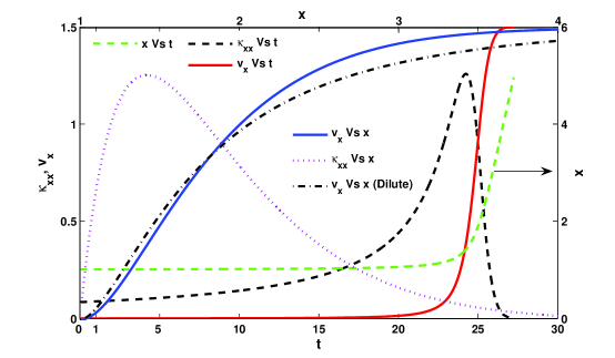
Figure 3: (Color online) Velocity $(v_{x})$ and velocity gradient $(\kappa_{xx})$ for an ultra-dilute solution (or a Newtonian fluid) along the center line in the wake of the cylinder, computed using the FEM formulation with the M5 mesh. The dashed green line is the position $x$, as a function of time, of a material particle traveling downstream starting close to the stagnation point. The dashed black line is the time dependent velocity gradient $\kappa_{xx}(t)$ used for carrying out BDS of the ultra-dilute models. The dot-dashed line is the velocity profile for a dilute Oldroyd-B model at $W\!i=0.6$.

The velocity field $v_{x}(x)$ and the velocity gradient $\kappa_{xx}(x)$ along the centerline, computed using the FEM formulation with the M5 mesh, are displayed in Fig. 3. Note the quadratic nature of the velocity close to the stagnation point. The position $x$ of a fluid packet as a function of time $t$, calculated using eqn (20), is displayed as the dashed green line. Consistent with the boundary conditions for the ODE for $\text{M}_{xx}$ above, we use $\delta=0.01$. Clearly, a material particle spends a significant fraction of time close to the stagnation point before rapidly accelerating away from it. The time dependent velocity gradient $\kappa_{xx}(t)$, necessary for the integration of the stochastic differential equation (18), calculated as described above, is shown as the dashed black line.

The configurational distribution function for the Hookean dumbbell model is Gaussian both at equilibrium, and in the presence of a homogenous flow field Bird et al. [1987b]. Since a Gaussian distribution is completely determined by its second moments, the initial distribution function at $x=1.01$ can be calculated for the known velocity gradient $\kappa_{xx}$, using the analytical solution for $\text{M}_{xx}$ in eqn (16) (and a similar expression for $\text{M}_{yy}$. Note $\text{M}_{zz}$ = 1). For Hookean dumbbells, the SDE (18) is integrated forward in time here, using a second order predictor-corrector Brownian dynamics simulation (BDS) algorithm Öttinger [1996], with an initial ensemble of connector vectors distributed according to the Gaussian distribution at $x=1.01$, subjected to the time dependent velocity gradient $\kappa_{xx}(t)$ for $t>0$.

The distribution function is also Gaussian in the case of the FENE-P model, and as a result, the initial distribution function at $x=1.01$ can in principle be determined using the second moments obtained by solving the set of governing equations (17). However, we adopt the simpler procedure of using a Gaussian distributed initial ensemble with equilibrium second moments, $\text{M}_{xx}=1$, $\text{M}_{yy}=1$, and $\text{M}_{zz}=1$, at $x=1.01$, since the solution of the SDE downstream of the stagnation point is found to be insensitive to the choice of the initial distribution. (For instance, identical results are obtained if the initial distribution of Hookean dumbbells at $x=1.01$, is used instead). The BDS algorithm for FENE-P dumbbells is identical to the one used to integrate the SDE for Hookean dumbbells, with the additional feature of having to evaluate ${\bigl{\langle}}{Q^{\dagger}}^{2}{\bigr{\rangle}}$ at every time step.

The exact (numerical) results along the centerline in the cylinder wake, for an ultra-dilute solution, calculated by solving the ODEs and the SDE above, are compared with the FEM solution in section IV below. Before doing so, however, important insights can be obtained by considering the nature of the maximum in the $\text{M}_{xx}$ component in the wake of the cylinder.

III.2 The maximum in the wake

For an ensemble of dumbbells which start near the stagnation point (where the velocity gradient $\kappa_{xx}$ is negligibly small), and then travel downstream to the region of fully developed flow (where $\kappa_{xx}=0$), the $\text{M}_{xx}$ component of the conformation tensor initially has a value close to unity, and ultimately returns to a value of unity. Since $\kappa_{xx}>0$ at intermediate values of $x$, it is clear that $\text{M}_{xx}$ must attain a maximum at some point $x=x^{*}$ along the centerline in the wake of the cylinder. Indeed all computations of flow around a confined cylinder report the occurrence of a maximum, and as mentioned earlier, failure to attain mesh convergence is usually observed most noticeably at the maximum.

At the maximum (where $d\text{M}_{xx}/{dx}=0$), eqn (15) implies that,

$$\text{M}_{xx}|_{x=x^{*}}=\frac{1}{1-2\,\lambda\kappa_{xx}|_{x=x^{*}}}$$ (21)

Clearly, if $\lambda\kappa_{xx}=0.5$ at $x=x^{*}$, the maximum value of $\text{M}_{xx}$ will be unbounded. One can see from the dotted curve in Fig. 3 that for values of $\lambda=\mathcal{O}(1)$, there are many points along the centerline in the cylinder wake where $\lambda\kappa_{xx}$ can be greater than 0.5. However, as manifest from eqn (21), the real issue is whether $\lambda\kappa_{xx}=0.5$ at $x=x^{*}$. This question is examined in the section below, using the different solutions methods discussed above.

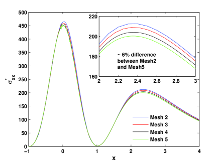
Figure 4: (Color online) The dimensionless polymer contribution to stress, $\sigma^{*}_{xx}=(\lambda/\eta_{\text{p,0}})\sigma_{xx}$, along the cylinder wall and along the centerline in the cylinder wake, at $W\!i=1.0$, for an ultra-dilute solution of an Oldroyd-B fluid. The computations are carried out using the FEM formulation discussed in section II.2. The inset shows the lack of mesh convergence in the wake.

IV Results and Discussion

IV.1 Ultra-dilute solutions

The failure to attain mesh convergence in the cylinder wake, for an ultra-dilute polymer solution at $W\!i=1$, using the FEM formulation discussed in section II.2, is displayed in terms of the non-dimensional polymer contribution to the stress in Fig. 4. The profile for the stress, with two maxima, one on the cylinder wall, and a second in the wake is typical for viscoelastic flow around a confined cylinder. As $W\!i$ increases further, the maximum in the wake grows significantly, and becomes the more dominant of the two maxima. The lack of mesh convergence, which is already apparent at $W\!i=1$ in Fig. 4, becomes much more pronounced. These predictions are completely in accord with what has been observed previously for dilute solutions. They have only been reproduced here to demonstrate the existence of a similar mesh convergence problem even in the simpler case of an ultra-dilute solution.

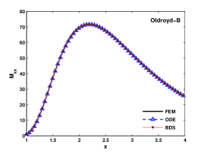
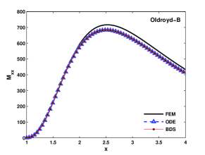
(a) $W\!i=0.8$	(b) $W\!i=1.3$
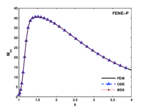
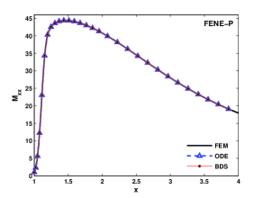
(c) $W\!i=1.5$	(d) $W\!i=2.0$

Figure 5: (Color online) The $\text{M}_{xx}$ component of the conformation tensor, computed using FEM, ODE and BDS, for an ultra-dilute solution of Oldroyd-B and FENE-P ($b=55$) fluids. The BDS results are obtained by averaging over $10^{6}$ dumbbell trajectories. The FEM results are computed using the M5 mesh. For the Oldroyd-B model, at $W\!i=1.3$, the FEM results at the maximum are approximately $6\%$ different from the ODE or BDS values.

The advantage of considering ultra-dilute solutions is that exact (numerical) solutions along the centerline in the cylinder wake can be obtained as outlined in section III.1. Fig. 5 compares the predictions of FEM computations with the exact solutions obtained by solving the ODEs, eqns (15) and (17), and by integrating (using BDS) the SDE, eqn (18), for the Oldroyd-B and FENE-P models. The excellent agreement of the FEM results with the exact solution (except for the Oldroyd-B model at $W\!i=1.3$) shows that the FEM results are accurate at the Weissenberg numbers that have been displayed. The departure of FEM predictions, at $W\!i=1.3$, from the exact results for the Oldroyd-B model (Fig. 5 (b)), is clear proof of the breakdown of FEM computations for $W\!i>1$. Since the exact solution is known for any value of $W\!i$, the error in the FEM computation can be estimated. Before we discuss the error, however, we first consider the more pressing issue of the value of the non-dimensional strain rate $\lambda\kappa_{xx}$ at $x=x^{*}$, the location of the maximum in $\text{M}_{xx}$ in the cylinder wake.

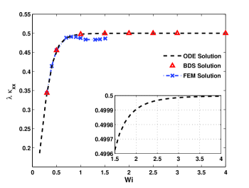
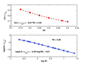
(a)	(b)

Figure 6: (Color online) (a) Dependence of the non-dimensional strain rate $\lambda\kappa_{xx}$ on $W\!i$, at the location $x=x^{*}$ of the maximum in $\text{M}_{xx}$ in the cylinder wake, for an ultra-dilute Oldroyd-B fluid. Inset shows $\lambda\kappa_{xx}|_{x=x^{*}}$ approaching $0.5$, computed from the ODE solution, for $W\!i>1.5$. (b) $\lambda\kappa_{xx}|_{x=x^{*}}$ approaches the critical value 0.5 as a power-law with increasing $W\!i$. The FEM results are for the M5 mesh and BDS results are obtained by averaging over $10^{6}$ individual Brownian trajectories of Hookean dumbbells.

Fig. 6 (a) displays $\lambda\kappa_{xx}|_{x=x^{*}}$ as a function of $W\!i$, for an ultra-dilute Oldroyd-B fluid, obtained with the three different solution techniques. As was discussed earlier in section III.2, the maximum in $\text{M}_{xx}$ becomes unbounded as $\lambda\kappa_{xx}|_{x=x^{*}}\to 0.5$ (see eqn (21)). Interestingly, $\lambda\kappa_{xx}|_{x=x^{*}}$ first approaches $0.5$ at $W\!i\approx 1$, where computational difficulties with the FEM method are first encountered. While the ODE solution and BDS can be continued to higher $W\!i$, FEM computations (indicated by the crosses) are no longer accurate beyond $W\!i=1$, breaking down completely by $W\!i=1.55$. This is related, as will be discussed in greater detail shortly, to the inability of the FEM solution to resolve the very large stresses that arise as $\lambda\kappa_{xx}|_{x=x^{*}}$ approaches 0.5. Fig. 6 (b) shows that the approach of $\lambda\kappa_{xx}|_{x=x^{*}}$ to the critical value is approximately linear in Weissenberg number for small values of $W\!i$, becoming a power-law ($W\!i^{-4.59}$), for $W\!i\gtrsim 0.4$. Thus, though $\lambda\kappa_{xx}|_{x=x^{*}}\to 0.5$ asymptotically, it never equals or exceeds the critical value. This implies that $\text{M}_{xx}$ (and, consequently, $\sigma^{*}_{xx}$) will increase without bound as $W\!i$ increases, but will never become singular.

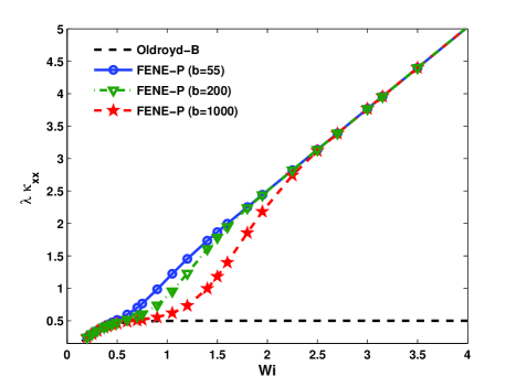
Figure 7: (Color online) Dependence of the non-dimensional strain rate $\lambda\kappa_{xx}$, at the location $x=x^{*}$ of the maximum in $\text{M}_{xx}$ in the cylinder wake, on $W\!i$, for a FENE-P fluid.

In the case of the FENE-P model, $\lambda\kappa_{xx}|_{x=x^{*}}$ approaches and exceeds 0.5 with increasing $W\!i$, as shown in Fig. 7, for a range of values of the finite-extensibility parameter $b$. The value 0.5 is not significant for the FENE-P model since, as can be seen from eqn (17), $\text{M}_{xx}|_{x=x^{*}}\rightarrow(b-\mathrm{tr}\,{\bf M}/{3})/(\mathrm{tr}\,{\bf M}/{3}-1)$ as $\lambda\kappa_{xx}|_{x=x^{*}}\to 0.5$. Hence, $\text{M}_{xx}|_{x=x^{*}}$ remains finite as long as $b$ is finite. Before we compare the predictions of $\text{M}_{xx}|_{x=x^{*}}$ and $\sigma^{*}_{xx}|_{x=x^{*}}$ by the Oldroyd-B and FENE-P models as a function of $W\!i$, it is interesting to consider the dependence of the location of the maximum, $x=x^{*}$, and $\kappa_{xx}|_{x=x^{*}}$, on $W\!i$.

Figure 8 (a) shows that for the Oldroyd-B model, the location $x^{*}$ of the maximum in $\text{M}_{xx}$ continuously moves downstream away from the stagnation point in the cylinder wake, with increasing $W\!i$. Simultaneously, Fig. 8 (b) indicates that the value of $\kappa_{xx}|_{x=x^{*}}$ continuously decreases. This is consistent with the behavior of $\kappa_{xx}$ as a function of $x$ displayed in Fig. 3. Since the velocity field is determined a priori for an ultra-dilute solution, $W\!i$ is varied in the computations by varying $\lambda$. With increasing $W\!i$, the product $\lambda\kappa_{xx}|_{x=x^{*}}$ (with $\lambda$ increasing, and $\kappa_{xx}|_{x=x^{*}}$ decreasing) tends to 0.5 in the manner depicted above in Fig. 6 (a). The continued use of the Oldroyd-B fluid in computational rheology, in spite of its known shortcoming in extensional flow, has sometimes been justified by the argument that real flows adapt to avoid an infinite stress. Curiously, the results in Figs. 6 and 8 appear to suggest that the flow does regulate the stress, and avoid a singularity. This does not, however, prevent the failure of the FEM computations for the Oldroyd-B fluid!

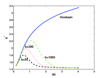
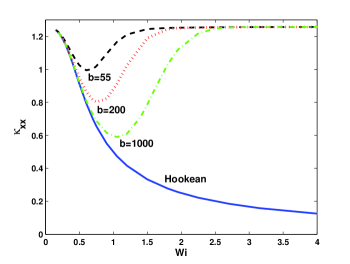
(a)	(b)

Figure 8: (Color online) The dependence on $W\!i$ of (a) the location $x^{*}$ of the maximum in $\text{M}_{xx}$, and (b) the strain rate $\kappa_{xx}|_{x=x^{*}}$, for ultra-dilute solutions of Oldroyd-B and FENE-P models. Results displayed are solutions of the respective ODEs.

For a FENE-P fluid, the location of the maximum in $\text{M}_{xx}$ and the value of $\kappa_{xx}$ at $x=x^{*}$, display intriguing behavior with increasing $W\!i$, as shown in Fig. 8. For each value of $b$, beyond some threshold value of $W\!i$, both quantities attain constant values. As a consequence, beyond this threshold value, the product $\lambda\kappa_{xx}|_{x=x^{*}}$ increases linearly with $W\!i$, as can be seen clearly in Fig. 7, enabling a straightforward mapping between $\lambda\kappa_{xx}|_{x=x^{*}}$ and $W\!i$ to be made.

The steep increase in $\text{M}_{xx}|_{x=x^{*}}$ and $\sigma^{*}_{xx}|_{x=x^{*}}$ for the Oldroyd-B model, as $\lambda\kappa_{xx}|_{x=x^{*}}\to 0.5$, is displayed in Figs. 9 (a) and (b). For the FENE-P model, there is a point of inflection at $\lambda\kappa_{xx}|_{x=x^{*}}=0.5$, after which the curves increase much more gradually with increasing $\lambda\kappa_{xx}|_{x=x^{*}}$. The shapes of the curves for the Oldroyd-B and FENE-P models are strikingly reminiscent of the well-known extensional viscosity versus strain rate curves for these models, commonly used to display the unphysical behavior of the Oldroyd-B model Bird et al. [1987b]; Owens and Phillips [2002]. As is well known, in that case, the onset of the steep increase in stress is attributed to the occurrence of a coil-stretch transition, leading to an unbounded stress in the Oldroyd-B model, but a bounded stress in the FENE-P model. While the former is because of the infinite extensibility of the Hookean spring in the Hookean dumbbell model, the latter is because of the existence of a upper bound to the mean stretchability of the spring in the FENE-P model. We can conjecture, consequently, that in the present instance also, polymer molecules undergo a coil-stretch transition in the wake of the cylinder, at the location of the stress maximum, giving rise to a stress that increases without bound as $W\!i$ increases.

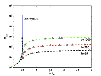
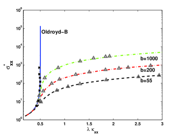
(a)	(b)

Figure 9: (Color online) Coil-stretch transition in the cylinder wake for an ultra-dilute solution. Dependence of the polymer stretch ($\text{M}_{xx}$) and stress ($\sigma^{*}_{xx}$), at $x=x^{*}$, on $\lambda\kappa_{xx}|_{x=x^{*}}$. The lines are ODE solutions and the symbols are FEM results on mesh M5.

The breakdown of the FEM computations for the Oldroyd-B model is clearly related to the steep increase in $\text{M}_{xx}|_{x=x^{*}}$ and $\sigma^{*}_{xx}|_{x=x^{*}}$, as $\lambda\kappa_{xx}|_{x=x^{*}}\to 0.5$. (Fig. 9 (b) indicates that the stress maximum increases by five orders of magnitude as $W\!i$ increases from 0.1 to 4). Since the exact solution is known at $x=x^{*}$, we can calculate the error at any value of $W\!i$ using,

$$\text{error}=\frac{(M^{\text{ODE}}_{xx}|_{x=x^{*}}-M^{\text{FEM}}_{xx}|_{x=x^{*}})}{M^{\text{ODE}}_{xx}|_{x=x^{*}}}\times 100$$ (22)

Error estimates obtained in this manner are displayed in Fig. 10 (a) for the Oldroyd-B model. The error remains small $(<1\%)$ at low $W\!i$, but increases sharply to approximately $8\%$ as $W\!i\gtrsim\mathcal{O}(1)$. The value of $W\!i^{*}$, the Weissenberg number up to which the error is less than $1\%$, depends on the degree of mesh refinement, and a clear improvement in $W\!i^{*}$ can be observed with increased mesh refinement. However, to obtain mesh converged results for $W\!i>0.7$ (with error $<1\%$), an approximately 100 fold increase in mesh density and hence, approximately $\sim 100$ fold increase in computational time is required.

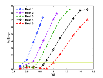
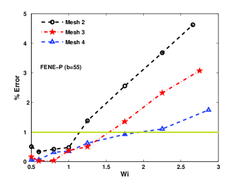
(a) Oldroyd-B	(b) FENE-P

Figure 10: (Color online) Percentage error in FEM computations of (a) $\text{M}_{xx}|_{x=x^{*}}$ for an ultra-dilute Oldroyd-B solution, and (b) $\text{M}_{yy}|_{x=x^{*}}$ for an ultra-dilute FENE-P fluid, as a function of $W\!i$. The error is calculated based on the results of the ODE solutions.

In the case of the FENE-P model, the error in $\text{M}_{xx}|_{x=x^{*}}$ is small even at relatively large values of $W\!i$ since the chains are close to their fully extended length, and it is difficult to see a clear pattern in the change in error with mesh refinement, unlike in the case of the Oldroyd-B model above. However, the error in the $\text{M}_{yy}|_{x=x^{*}}$ component reveals a more systematic behavior, as displayed in Fig. 10 (b), with a decrease in error with increasing mesh refinement.

The infeasibility of carrying out FEM computations for the confined flow around a cylinder of an ultra-dilute Oldroyd-B fluid, for $W\!i>1$, is revealed in Fig. 11, where the exponential increase in the number of elements required to attain an error less than $1\%$, with increasing $W\!i$, can be clearly observed. For the FENE-P model, the rate of increase in the number of elements required for an error less than $1\%$ is significantly lower than that for the Oldroyd-B fluid. The Mesh 4 curve in Fig. 10 (b) even seems to suggest that there might be a degree of mesh refinement beyond which, for the FENE-P model, one can compute at any $W\!i$ with an error less than $1\%$. However, this trend is not easily discernible in Fig. 11, and addtional mesh refinement may be required before a firm conclusion can be drawn. Further, a change of variable to the matrix logarithm of the conformation tensor, may lead to mesh converged results at significantly higher vales of $W\!i$.

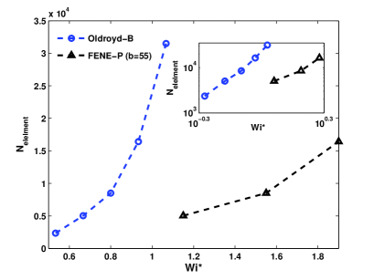
Figure 11: (Color online) The number of elements as a function of the Weissenberg number $W\!i^{*}$, up to which the error remains less than $1\%$, for the Oldroyd-B and FENE-P models. The inset displays the same data as a log-log plot.

The reason polymer molecules undergo a coil-stretch transition as they travel down the centerline in the cylinder wake is because of the extended period of time they spend in the neighborhood of the stagnation point, which leads to a significant accumulation of strain. The Hencky strain $\epsilon$ at any instant $t$, calculated from the expression $\epsilon=\int_{0}^{t}dt^{\prime}\,\kappa_{xx}(t^{\prime})$, is displayed in Fig. 12. A very large Hencky strain of roughly 8 units is built up by the time the molecules approach $x^{*}$. For a material element of unit length at $t=0$, this corresponds to a ratio of final to initial length of roughly 3000. The behavior of individual molecules as they are subjected to this degree of straining can be obtained, for an ultra-dilute solution, from the Brownian dynamics simulations carried our here since one can calculate the trajectories of dumbbells as they are convected by the flow field down the centerline, subjected to the local strain rate.

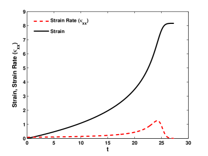
Figure 12: (Color online) Hencky strain accumulated by a fluid element as it travels along the centerline, from the neighborhood of the stagnation point in the cylinder wake.

In this context, it is instructive to calculate the size of individual dumbbells relative to a macroscopic feature, such as the length of an element in the finite element mesh. In the non-dimensionalization scheme used here, however, since the macroscopic length scale is the cylinder radius $a$, and the microscopic length scale for Hookean dumbbells is $\sqrt{{\bigl{\langle}}Q^{2}{\bigr{\rangle}}_{\text{eq}}/3}$, direct comparison is difficult unless one has estimates of these length scales. Here, we use the experimental data of McKinley et al. [1993], who investigated the flow around a confined cylinder (with radius $3.188\times 10^{-3}\,\text{m}$) of a 1.2 million molecular weight Polyisobutelene solution, to obtain a typical estimate of these length scales. For these molecules, the equilibrium size can be shown to be $\sqrt{{\bigl{\langle}}Q^{2}{\bigr{\rangle}}_{\text{eq}}}=0.0497\,\mu\text{m}$. Defining a dimensionless length in the flow direction by,

$$Q^{*}_{x}=\frac{Q^{\dagger}_{x}\,\sqrt{{\bigl{\langle}}Q^{2}{\bigr{\rangle}}_{\text{eq}}/3}}{a\,L_{m}|_{x=x^{*}}}$$ (23)

where, $L_{m}|_{x=x^{*}}$ is the non-dimensional length of the element at $x=x^{*}$, the relative length of individual molecules in the flow direction can be calculated from the BDS trajectories as a function of strain.

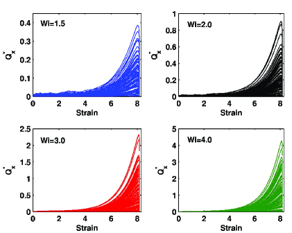
Figure 13: (Color online) The length of individual polymer molecules relative to the size of an element of the M5 mesh, at $x=x^{*}$, at various values of $W\!i$, for an ultra-dilute Oldroyd-B fluid. The experimental data of McKinley et al. [1993] is used to obtain an estimate of the equilibrium size of the molecules and the cylinder radius.

Figures 13 display $Q^{*}_{x}$ as a function of $\epsilon$, for an ensemble of 100 dumbbell trajectories, at various values of $W\!i$. Nearly all the dumbbells appear to remain close to their initial state of extension until approximately 5 strain units, beyond which several of the dumbbells undergo rapid extension, which is more pronounced as $W\!i$ increases. The rapid extension of the dumbbell spring represents the physical unraveling of a polymer molecule from a coiled to a stretched state, and the results in Figs. 13 are inline with the notion that a coil-stretch transition occurs as the molecules experience the maximum strain. As expected, the molecules relax back to their equilibrium configurations once the strain rate downstream of the maximum becomes zero.

The use of the local element size to achieve non-dimensionalization reveals strikingly that the magnitude of some of the molecules is large enough to span several elements. Kinetic theory models, such as the Hookean dumbbell model, are typically built on the assumption of homogenous fields, with negligible variation on the length scale of individual molecules. The data in Figs. 13 suggests that the extensive use of the unphysical Oldroyd-B model in complex flow simulations is questionable, and highlights the need to derive more refined models that are valid in non-homogeneous fields.

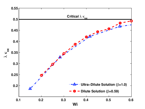
Figure 14: (Color online) Dependence of $\lambda\kappa_{xx}|_{x=x^{*}}$ on $W\!i$ for dilute and ultra-dilute solutions. The dilute solution curve first approaches the critical value at a value of $W\!i$ at which difficulties with FEM computations usually arise.

IV.2 Dilute solutions

All the results reported so far have been for ultra-dilute models, where the existence of exact solutions has enabled us to obtain a variety of insights into the origin of difficulties encountered with FEM computations. There is already an extensive literature on the numerical computation of the flow around a confined cylinder of various dilute solution models, and there are no new numerical techniques introduced in this paper for us to be able to report an improvement in the maximum attainable mesh converged Weissenberg number. Our interest here, instead, is to examine if any of the insight that has been gained for ultra-dilute solutions can be used to understand the observed behavior of dilute solutions.

The coupling of the velocity and the conformation tensor (and stress) fields, makes it impossible to obtain exact solutions for these variables. As a result, it is not possible to obtain error estimates as in the case of ultra-dilute solutions, or to calculate the trajectories of individual dumbbell molecules convected along the centerline by the flow. Nevertheless, we can exploit the key insight of the previous section because the value of the maximum in the $\text{M}_{xx}$ component in the cylinder wake, for the Oldroyd-B model, is still given by eqn. (21), even though we do not have a pre-determined velocity field $v_{x}(x)$.

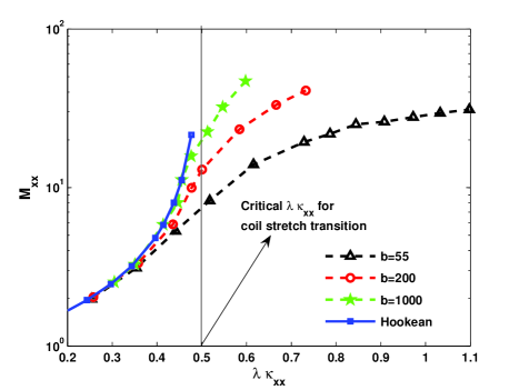
Figure 15: (Color online) Coil-stretch transition in the cylinder wake for a dilute solution. Variation of the polymer stretch $\text{M}_{xx}$ with $\lambda\kappa_{xx}|_{x=x^{*}}$ for Oldroyd-B and FENE-P models. The M4 mesh is used for the Oldroyd-B model and the M3 mesh is used for the FENE-P model in FEM computations. The viscosity ratio $\beta=0.59$.

In the case of an ultra-dilute solution, it was relatively straightforward to find the location $x^{*}$ of the stress maximum in the cylinder wake for each value of $W\!i$, and to calculate $\lambda\kappa_{xx}|_{x=x^{*}}$ from the known velocity field. For a dilute solution, the velocity field changes with each change in $W\!i$. All the same, it is still possible to find $\lambda\kappa_{xx}|_{x=x^{*}}$, at various values of $W\!i$, by integrating the full system of equations for the velocity and conformation tensor fields using the FEM formulation. A typical velocity profile for a dilute solution at $W\!i=0.6$ is shown in Fig. 3 as the dot-dashed line. (At this value of $W\!i$, it can be seen that the velocity profile is not significantly different from that for an ultra-dilute solution.)

Figure 14 indicates that $\lambda\kappa_{xx}|_{x=x^{*}}$ for a dilute solution approaches the critical value of 0.5 in a manner similar to that of an ultra-dilute solution, albeit at a slightly more rapid rate with increasing $W\!i$. The curve is not as smooth as the ultra-dilute case because of the growing error in FEM computations as $W\!i$ reaches the upper limit of computable values. Indeed, the typical limit of $W\!i=0.6$ where most computations in the literature first encounter problems, appears to be the value at which $\lambda\kappa_{xx}|_{x=x^{*}}$ first comes close to 0.5.

As may be anticipated from eqn. (21), $\text{M}_{xx}$ and $\sigma^{*}_{xx}|_{x=x^{*}}$ will increase steeply for the Oldroyd-B model as $\lambda\kappa_{xx}|_{x=x^{*}}\to 0.5$. This can be seen very clearly from Fig. 15, where $\text{M}_{xx}$ appears to become unbounded in this limit. For the FENE-P fluid on the other hand, the curves for $\text{M}_{xx}$ exhibit a point of inflection at $\lambda\kappa_{xx}|_{x=x^{*}}=0.5$, before leveling off to the fully stretched value corresponding to the respective value of $b$.

The similarity of the shapes of the curves in Fig. 15 to the curves in Fig. 9, and to the well-known extensional viscosity versus strain rate curves for the Oldroyd-B and FENE-P models suggests that even for a dilute solution, there occurs a coil-stretch transition at the location of the stress maximum in the cylinder wake, and this coil-stretch transition is the source of problems encountered with FEM computations for the flow of an Oldroyd-B fluid around a confined cylinder. It would be of great interest to examine if a similar coil-stretch transition is the source of computational difficulties encountered in the numerical simulation of other benchmark complex flows of Oldroyd-B fluids.

V Conclusions

The flow around a cylinder confined between parallel plates, of ultra-dilute and dilute polymer solutions, modeled by the Oldroyd-B and FENE-P constitutive equations, has been considered with a view to understand the origin of computational difficulties encountered in numerical simulations.

FEM computations of ultra-dilute Oldroyd-B solutions are shown to breakdown at $W\!i=\mathcal{O}(1)$, as has been observed previously for dilute solutions (see Fig. 4). Two different numerical means of obtaining an exact solution along the centerline in the cylinder wake, for both the Oldroyd-B and the FENE-P models, have been developed to enable a careful examination of the causes of the breakdown. The exact solution techniques, namely solving a system of ODEs and carrying out Brownian dynamics simulations, are useful to evaluate the value of $W\!i$ up to which the FEM computations are accurate (see Figs. 5), and to estimate the error in the FEM results (see Figs. 10).

An analysis of the structure of the Oldroyd-B equation shows that the maximum in the $\text{M}_{xx}$ component of the conformation tensor along the centerline in the cylinder wake, becomes unbounded if the non-dimensional strain rate at the location of the stress maximum, $\lambda\kappa_{xx}|_{x=x^{*}}$, approaches a critical value of $0.5$ (see eqn (21)). Numerical solution of the governing equations for an ultra-dilute solution reveals that $\lambda\kappa_{xx}|_{x=x^{*}}\to 0.5$ as a power-law in $W\!i$, for $W\!i\gtrsim\mathcal{O}(1)$ (see Fig. 6 (a) and (b)). On the other hand, analysis of the FENE-P model reveals that the maximum in $\text{M}_{xx}$ remains bounded for all values of the local non-dimensional strain rate. In contrast to the Oldroyd-B model, numerical results for $\lambda\kappa_{xx}|_{x=x^{*}}$ show that it does not have an asymptotic value, but instead increases linearly with $W\!i$ beyond a threshold value of the Weissenberg number (see Fig. 7).

As $\lambda\kappa_{xx}|_{x=x^{*}}\to 0.5$, both the maximum in $\text{M}_{xx}$ and the maximum in the stress ($\sigma^{*}_{xx}$) increase without bound for the ultra-dilute Oldroyd-B model. In comparison, for an ultra-dilute FENE-P model, these variables increase relatively rapidly as $\lambda\kappa_{xx}|_{x=x^{*}}$ approaches 0.5, but level off and remain bounded for higher values of $\lambda\kappa_{xx}|_{x=x^{*}}$ (see Figs. 9). The shape of the curves are strongly suggestive of the occurrence of a coil-stretch transition in the cylinder wake.

The steep increase in $\text{M}_{xx}$ and $\sigma^{*}_{xx}$ in the vicinity of $W\!i=\mathcal{O}(1)$ necessitates the use of increasingly refined meshes for increasing values of $W\!i$. The number of elements required to maintain the error in $\text{M}_{xx}$ less than 1% is shown to increase exponentially with increasing $W\!i$ for the Oldroyd-B model, making it practically infeasible to obtain solutions at $W\!i>1$. In the case of the FENE-P model, the current simulation data is inadequate to draw firm conclusions (see Figs. 11).

A material element of an ultra-dilute solution is shown to accumulate nearly 8 units of Hencky strain as it travels downstream from the stagnation point in the wake of the cylinder, due to the extended time it spends in the vicinity of the stagnation point (see Fig. 12). This strain leads to dumbbells undergoing a large extension in the flow direction, with their magnitude large enough to span several elements in the local finite element mesh see Fig. 13).

The analysis of the nature of the maximum in $\text{M}_{xx}$ in the cylinder wake, which suggests that the maximum becomes unbounded if $\lambda\kappa_{xx}|_{x=x^{*}}$ approaches the critical value of $0.5$, is valid for both ultra-dilute and dilute Oldroyd-B fluids. FEM computations of the fully coupled governing equations for a dilute Oldroyd-B fluid have been carried out to show that, just as in the case of an ultra-dilute solution, $\lambda\kappa_{xx}|_{x=x^{*}}$ tends to 0.5 with increasing $W\!i$ (see Fig. 14). The approach, however, is more rapid than the ultra-dilute case, with $\lambda\kappa_{xx}|_{x=x^{*}}$ becoming nearly equal to 0.5 at $W\!i\approx 0.6$, the value of the Weissenberg number where computational difficulties have been reported in the literature to be first typically encountered.

The approach of $\lambda\kappa_{xx}|_{x=x^{*}}$ to the critical value is shown to be accompanied by an unbounded increase in the maximum values of $\text{M}_{xx}$ and $\sigma^{*}_{xx}$ in the cylinder wake for a dilute Oldroyd-B fluid. FEM computations of the coupled governing equations for a FENE-P fluid on the other hand show that these variables increase relatively rapidly close to $\lambda\kappa_{xx}|_{x=x^{*}}=0.5$, but level off and remain bounded at higher values (see Figs. 15). The similarity of the curves with observations for ultra-dilute solutions, is strong evidence for a coil-stretch transition also occurring in dilute solutions, in the wake of the cylinder at the location of the stress maximum.

Several issues that must be addressed in the future can be tackled fruitfully with the framework developed here. For instance, the nature and structure of stress boundary layers in the vicinity of the cylinder can be examined for ultra-dilute solutions along lines similar to the analysis here. Further, the existence of a coil-stretch transition suggests that a model with conformation dependent drag might reveal the existence of coil-stretch hysteresis in the cylinder wake.

Acknowledgements This work has been supported by a grant from the Australian Research Council under the Discovery-Projects program, and the National Science Foundation. The authors would like to thank the APAC, VPAC (Australia) and the RTC (Rice University, Houston) for the allocation of computing time on their supercomputing facilities. JRP acknowledges helpful discussions with Professors Eric Shaqfeh and Gareth McKinley.

References

- Alves et al. [2001] Alves, M. A., F. Pinho and P. J. Oliveira, “The flow of viscoelastic fluids past a cylinder: finite-volume high-resolution methods,” J. Non-Newtonian Fluid Mech. 97, 207–203 (2001).
- Bird et al. [1987a] Bird, R. A., R. C. Armstrong and O. Hassager, Dynamics of Polymeric Liquids, vol. 1, John Wiley & Sons, New York, 2nd edn. (1987a).
- Bird et al. [1987b] Bird, R. A., C. F. Curtiss, R. C. Armstrong and O. Hassager, Dynamics of Polymeric Liquids, vol. 2, John Wiley & Sons, New York, 2nd edn. (1987b).
- Caola et al. [2001] Caola, A. E., Y. L. Yoo, R. C. Armstrong and R. A. Brown, “Highly parallel time integration of viscoelastic flows,” J. Non Newt. Fluid Mech. 100, 191–216 (2001).