Mott insulating phases and quantum phase transitions of interacting spin-$\frac{3}{2}$ fermionic cold atoms in optical lattices at half filling

Abstract

We study various Mott insulating phases of interacting spin-$\frac{3}{2}$ fermionic ultracold atoms in two-dimensional square optical lattices at half filling. Using a generalized one-band Hubbard model with hidden SO(5) symmetry, we identify two distinct symmetry breaking phases: the degenerate antiferromagnetic spin-dipole/spin-octupole ordering and spin-quadrupole ordering, depending on the sign of the spin-dependent interaction. These two competing orders exhibit very different symmetry properties, low energy excitations and topological characterizations. Near the SU(4) symmetric point, a quantum critical state with a $\pi$-flux phase may emerge due to strong quantum fluctuations, leading to spin algebraic correlations and gapless excitations.

I Introduction

The Mott insulating states are attracting extensive attention in modern condensed matter physics, which are believed to play a crucial role for resolving the mysteries in high temperature superconductors, heavy fermion compounds, colossal magnetoresistance manganites and so on. In the conventional band theory, the insulators are characterized by an energy gap between the highest filled and the lowest empty states. On the other hand, a charge excitation gap can open up with a partially filled energy band due to the competition between kinetic energy and repulsive force between the particles. Since the strong correlation effects are difficult to handled, an efficient theoretical description of the Mott insulating states is still a challenging task.

Since Greiner et al. experimentally succeeded in observing the superfluid-Mott phase transition of ultracold bosonic atoms in optical lattices Bloch-2002 , studying strongly interacting cold atom systems becomes a new research direction of condensed matter physics. In fact, an atomic Mott insulator is prepared using a deep optical lattice, where the particle number fluctuations are strongly suppressed. Such systems are rather clean and controllable compared to conventional solid state systems. Besides the single component atoms, the spinor atoms can also be loaded into the optical traps or lattices, leading to a variety of novel quantum phenomena.

Depending on the hyperfine spin values, the ultracold atoms are classified as bosons with integer $F$ and fermions with half odd $F$. Most previous studies on the Mott insulating states focused on scalar and spinor bosonic atoms. Various Mott insulating phases are also formed in higher spin ultracold atoms in optical lattices. For spin-1 bosons, the spin-singlet, dimerized, and the nematic Mott insulating states were studied Demler-Zhou-2002 ; Yip-2003 ; Zhou-2003 ; Demler-2003 ; Bernier-Kim-2006 . For spin-2 bosons, even more complicated Mott insulators can be realized Zhou-2006 ; Eckert-2006 . Depending on the scattering length and particle occupation number per site, the ground state can be spin-ordered ferromagnetic, cyclic and nematic states. When the potential barriers of the optical lattices are very high, one can even observe the coherent spin-mixing oscillations of the two isolated spin-2 ⁸⁷Rb atoms in one site Bloch-2005 ; HJHuang-2006 . Recently, the Mott insulating phases of spin-3 ⁵²Cr atoms have attracted attention motivated by the experimental progress, where the long-range dipole interaction plays an important role in determining the exotic ground states Bernier-2006 .

Actually, the physics of fermionic ultracold atoms in optical lattices is also interesting. For spin-$\frac{1}{2}$ fermions, the Hubbard and $t-J$ like models can be realized in optical lattices, which may shed light on the fundamental issues in studying the high-$T_{c}$ superconductors in the doped cuprates klein-jaksch . Furthermore, the high spin fermionic atoms provide opportunities to study novel basic physics with no counterparts for electrons in solids. Recently, rare-earth ¹⁷³Yb atoms with the lowest hyperfine manifold $F=\frac{5}{2}$ have been cooled down to quantum degeneracy regime Takahashi-2007 , free of spin relaxation. On the other hand, the $F=\frac{3}{2}$ interacting fermionic system is attracting theoretical interest, which can be realized with alkali atoms ¹³²Cs, as well as alkaline-earth atoms ⁹Be, ¹³⁵Ba, and ¹³⁷Ba. Recently, Wu et al. noticed that the spin-$\frac{3}{2}$ fermions with $s$-wave scattering interaction enjoy a hidden SO(5) symmetry, without tuning any parameter CWu-2003 ; CWu-2006 . Then, more interesting issues are studied, such as the competition between the baryon-like quartet pairing state and quintet pairing state in one-dimension CWu-2005 , the topological generation of quantum entanglement by non-Abelian half quantum vortices in quintet superfluid phase CWu-Hu-2005 .

In this paper, we will investigate the various Mott-insulating states and map out the ground state phase diagram for a half filled spin-$\frac{3}{2}$ ultracold fermionic atom system on a two dimensional square optical lattice. In addition to the spin-quadrupole ordering state Tu-2006 , we will show that a new Mott insulating state with degenerate antiferromagnetic spin-dipole/spin-octupole ordering can be formed as well. Between these two distinct spin-ordered phases, an SU(4) $\pi$-flux state may emerge as a quantum critical phase due to the competing orders. Furthermore, the spin-quadrupole correlations, as well as the spin-dipole and spin-octupole correlations display the same power-law behavior. This is in analogy with the staggered flux state in quantum spin $S=\frac{1}{2}$ Heisenberg antiferromagnets, in which the competing Néel order parameter and the valence-bond solid order parameter exhibit the same power-law correlations. In fact, the SU(4) $\pi$-flux state and the SU(2) staggered flux state both belong to a class of algebraic spin liquid states that unify the competing orders by emergent symmetry at low energies Hermele-2005 . A variety of novel algebraic spin liquid states have been studied in the underdoped region of cuprates Rantner-2001 , toy spin models Moessner-2003 ; Wen-2003 ; Hermele-2003 ; Xu-2006 and strongly correlated p-orbital band bosons in optical lattices Xu-Fisher-2006 .

The paper is organized as follows. In Sec. II, the general spin-$\frac{3}{2}$ Hubbard model will be introduced, which describes the spin-$\frac{3}{2}$ interacting fermionic atoms in optical lattices. In Sec. III, we will briefly review the Mott insulating phase with a staggered spin-quadrupole order. In Sec. IV, the Mott insulating phase with degenerate antiferromagnetic spin-dipole/spin-octupole order will be studied within the functional integral approach. The corresponding symmetry breaking pattern and the low energy collective excitation modes are discussed. Sec. V is devoted to an analysis of the SU(4) $\pi$-flux state as a quantum critical state. The phase diagram is obtained based on an effective model at low energies. Finally, a brief discussion is presented in Sec. VI.

II Generalized one-band Hubbard model

An optical lattice is a periodic potential $V(\mathbf{r})=\sum_{r=x,y,z}V_{r}\sin^{2}(\mathbf{k\cdot r})$ created by standing-wave laser beams, where $|\mathbf{k}|=2\pi/\lambda$ is the wave vector of the laser and $\lambda/2$ is the lattice spacing. When the potential is tuned to $V_{z}\gg V_{x}=V_{y}$, the atoms are confined to the lowest Bloch band of a two-dimensional $x$-$y$ plane square lattice at low temperatures. The system of spin-$\frac{3}{2}$ ultracold interacting fermionic atoms is well described by a generalized one-band Hubbard model

$$H = -t\sum_{\langle ij\rangle}(\psi_{i}^{{\dagger}}\psi_{j}+\text{H.c.})+\frac{c_{0}}{2}\sum_{i}(N_{i}-2)^{2}$$ (1)

$$+\frac{c_{2}}{2}\sum_{i}\mathbf{S}_{i}^{2}-\mu\sum_{i}N_{i},$$

where $\psi$ is a four-component spinor defined by $\psi_{i}=\left(\psi_{i,3/2},\psi_{i,1/2},\psi_{i,-1/2},\psi_{i,-3/2}\right)^{T}$ and the chemical potential $\mu=0$ is fixed at half filling on a bipartite lattice. Within the harmonic approximation, the parameters for the two-dimensional square optical lattice are given by

$$t = \frac{2}{\sqrt{\pi}}E_{R}\xi^{3}\exp(-2\xi^{2}),$$

$$c_{0} \sim \frac{5a_{2}-a_{0}}{\lambda}E_{R}\xi^{3},$$

$$c_{2} \sim \frac{a_{2}-a_{0}}{\lambda}E_{R}\xi^{3},$$ (2)

where $E_{R}=\hbar k^{2}/2m$ is the recoil energy, $\xi=(V_{x}/E_{R})^{1/4}$ and $a_{S}$ is the $s$-wave scattering length in the total spin-$S$ channel. Due to the Pauli’s exclusion principle, the $s$-wave interactions of identical spin-$\frac{3}{2}$ fermions in total spin $S=1$, $3$ channels are forbidden. The particle number and spin operators at lattice site $i$ are defined by

$$N_{i}=\sum_{\alpha}\psi_{i\alpha}^{{\dagger}}\psi_{i\alpha},\text{ }\mathbf{S}_{i}=\sum_{\alpha\beta}\psi_{i\alpha}^{{\dagger}}\mathbf{S}_{\alpha\beta}\psi_{i\beta},$$ (3)

where $\mathbf{S}$ are the spin-$\frac{3}{2}$ matrices. In addition, we have to consider the higher-order products of the spin matrices. The spin-quadrupole matrices are defined by

$$\frac{1}{\sqrt{3}}\left(S^{x}S^{y}+S^{y}S^{x}\right) = \Gamma^{1},\text{ }\frac{1}{\sqrt{3}}\left(S^{z}S^{x}+S^{x}S^{z}\right)=\Gamma^{2},$$

$$\frac{1}{\sqrt{3}}\left(S^{z}S^{y}+S^{y}S^{z}\right) = \Gamma^{3},\text{ }\left(S^{z}\right)^{2}-\frac{5}{4}=\Gamma^{4},$$

$$\frac{1}{\sqrt{3}}\left[(S^{x})^{2}-(S^{y})^{2}\right] = \Gamma^{5},$$ (4)

where

$$\Gamma^{1}=\left(\begin{array}[]{cc}0&-iI\\ iI&0\end{array}\right),\Gamma^{2,3,4}=\left(\begin{array}[]{cc}\vec{\sigma}&0\\ 0&-\vec{\sigma}\end{array}\right),\Gamma^{5}=\left(\begin{array}[]{cc}0&I\\ I&0\end{array}\right),$$

are the five Dirac Gamma matrices satisfying the Clifford algebra $\{\Gamma^{a},\Gamma^{b}\}=2\delta_{ab}$, $I$ is a $2\times 2$ unit matrix and $\vec{\sigma}$ are Pauli matrices. In terms of $\Gamma$ matrices, we have also tensor operators defined by $\Gamma^{ab}=-\frac{i}{2}[\Gamma^{a},\Gamma^{b}]$. Thus, the spin-$\frac{3}{2}$ (dipole) matrices are expressed as linear combinations of $\Gamma^{ab}$:

$$S^{x} = \frac{\sqrt{3}}{2}\Gamma^{34}+\frac{1}{2}(\Gamma^{12}+\Gamma^{35}),$$

$$S^{y} = -\frac{\sqrt{3}}{2}\Gamma^{24}-\frac{1}{2}(\Gamma^{13}-\Gamma^{25}),\text{ }$$

$$S^{z} = -\Gamma^{15}+\frac{1}{2}\Gamma^{23},$$ (5)

which form the spin SU(2) algebra with $[S^{\alpha},S^{\beta}]=i\epsilon_{\alpha\beta\gamma}S^{\gamma}$. Moreover, there are seven spin-octupole matrices given by

$$(S^{x})^{3} = \frac{7\sqrt{3}}{8}\Gamma^{34}+\frac{7}{8}\Gamma^{35}+\frac{13}{8}\Gamma^{12},$$

$$(S^{y})^{3} = -\frac{7\sqrt{3}}{8}\Gamma^{24}+\frac{7}{8}\Gamma^{25}-\frac{13}{8}\Gamma^{13},$$

$$(S^{z})^{3} = \frac{13}{8}\Gamma^{23}-\frac{7}{4}\Gamma^{15},$$

$$\{S^{x},(S^{y})^{2}-(S^{z})^{2}\} = -\frac{\sqrt{3}}{2}\Gamma^{34}+\frac{3}{2}\Gamma^{35},$$

$$\{S^{y},(S^{z})^{2}-(S^{x})^{2}\} = -\frac{\sqrt{3}}{2}\Gamma^{24}-\frac{3}{2}\Gamma^{25},$$

$$\{S^{z},(S^{x})^{2}-(S^{y})^{2}\} = \sqrt{3}\Gamma^{14},$$

$$S^{x}S^{y}S^{z}+S^{z}S^{y}S^{x} = \frac{\sqrt{3}}{2}\Gamma^{45},$$ (6)

where we have used the abbreviation $\left\{A,B\right\}=AB+BA$. The spin-quadrupole operators, spin-dipole and spin-octupole operators can be simply expressed as

$$n_{i}^{a} = \frac{1}{2}\sum_{\alpha\beta}\psi_{i\alpha}^{{\dagger}}\Gamma_{\alpha\beta}^{a}\psi_{i\beta}\;(1\leq a\leq 5),$$ (7)

$$L_{i}^{ab} = -\frac{1}{2}\sum_{\alpha\beta}\psi_{i\alpha}^{{\dagger}}\Gamma_{\alpha\beta}^{ab}\psi_{i\beta}\;(1\leq a<b\leq 5),$$ (8)

where $n_{i}^{a}$ corresponds to an SO(5) superspin vector, and $L_{i}^{ab}$ constitute the adjoint representation of the SO(5) Lie group satisfying the commutation relations:

$$[L_{i}^{ab},L_{j}^{cd}]=i\delta_{ij}(\delta_{ad}L_{i}^{bc}+\delta_{bc}L_{i}^{ad}-\delta_{ac}L_{i}^{bd}-\delta_{bd}L_{i}^{ac}).$$ (9)

Furthermore, $n_{i}^{a}$ and $L_{i}^{ab}$ together as generators form an SU(4) Lie group, the highest symmetry group for four-component spin-$\frac{3}{2}$ fermions in the particle-hole channel. Under the SO(5) transformations, the sixteen bilinear operators in the particle-hole channel are classified as particle number operator (scalar), spin-quadrupole operators (vector), spin-dipole and spin-octupole operators (tensor).

We would like to emphasize that in the multipolar expansion of classical electrodynamics, the higher-order multipolar interactions are usually much weaker than the dipolar interactions. However, this is not the case in the present system, where spin dipolar and multipolar operators are all expressed in terms of bilinear combinations of the fermionic operators.

In this paper, we will focus on the Mott insulating phases with two atoms per site. In the limit of $t=0$, each lattice site decouples from its nearest neighbor sites, then the single site ground state is a spin singlet ($S_{i}=0$) for $c_{2}>0$ and a spin quintet ($S_{i}=2$) for $c_{2}<0$. For $c_{2}=0$, the ground state is a six-fold degenerate state and the interactions gain an enhanced SU(4) symmetry. Since the scattering lengths for the spin-$\frac{3}{2}$ fermionic ultracold atoms are not available yet, we consider the parameter regime of $c_{0}\gg|c_{2}|,t$, where the spin-dependent interaction are much weaker than the spin-independent one. Actually, this request is well satisfied for current alkali atom experiments. Under these considerations, the stability of Mott insulator with double occupancy is also guaranteed and an interesting phase diagram with three different kinds of Mott insulating states will be obtained.

III Spin-quadrupole ordering state

In this section, we briefly review the Mott insulating phase with staggered spin-quadrupole ordering formed by the half-filled spin-$\frac{3}{2}$ fermionic atoms in a two-dimensional optical lattice Tu-2006 . To reveal such an order, the generalized Hubbard model can be rewritten in an SO(5) invariant form CWu-2003

$$H = -t\sum_{\langle ij\rangle,\alpha}(\psi_{i\alpha}^{{\dagger}}\psi_{j\alpha}+\text{H.c.})-\frac{3c_{2}}{4}\sum_{i,1\leq a\leq 5}(n_{i}^{a})^{2}$$ (10)

$$+\frac{8c_{0}-15c_{2}}{16}\sum_{i}(N_{i}-2)^{2}-\mu\sum_{i}N_{i}.$$

Provided the commutation rules

$$[L_{i}^{ab},n_{j}^{c}]=i\delta_{ij}(\delta_{bc}n_{i}^{a}-\delta_{ac}n_{i}^{b})$$ (11)

are satisfied, the generic SO(5) symmetry of this model manifests explicitly, i.e., the Hamiltonian is invariant under the transformation

$$\psi\rightarrow\psi^{\prime}=e^{-iL^{ab}\theta_{ab}}\psi,\text{ }1\leq a<b\leq 5,$$ (12)

where $\theta_{ab}$ are the Euler angles representing infinitesimal rotations between the ten independent planes in five dimensions. At half filling, the chemical potential $\mu$ is zero and the average number of fermions per site is $\langle N_{i}\rangle=2$. As far as an insulating state is concerned, the particle number fluctuations can be neglected and we focus on the quantum spin fluctuations, which result in various spin ordering states. In particular, for $c_{2}>0$, site-singlets formed by two spin-$\frac{3}{2}$ fermions with total spin $S=0$ are energetically favorable. In this case, the quantum spin-quadrupole fluctuations are an important feature of the generalized Hubbard model. As we have shown in the previous work Tu-2006 , the doubly occupied fermionic atoms in a square lattice can exhibit a staggered spin-quadrupole ordering with the order parameter $(-1)^{i}\langle n_{i}^{a}\rangle\neq 0$. Without loss of generality, the order parameter can be chosen as $(-1)^{i}\langle n_{i}^{4}\rangle\neq 0$, where

$$2n_{i}^{4}=\psi_{i,\frac{3}{2}}^{\dagger}\psi_{i,\frac{3}{2}}+\psi_{i,-\frac{3}{2}}^{\dagger}\psi_{i,-\frac{3}{2}}-\psi_{i,\frac{1}{2}}^{\dagger}\psi_{i,\frac{1}{2}}-\psi_{i,-\frac{1}{2}}^{\dagger}\psi_{i,-\frac{1}{2}},$$ (13)

corresponding to the difference between the $S^{z}=\pm 3/2$ and $S^{z}=\pm 1/2$ spin densities in the site singlet state. The typical configuration of this particular spin-quadrupole ordering state is shown in Fig. 1. This quantum analogue of liquid crystal state breaks the spin SU(2) rotational symmetry, but preserves the time reversal symmetry.

Due to the fixed direction $n_{i}^{4}$ of the SO(5) superspin vector, the symmetry of the spin-quadrupole ordering ground state is spontaneously broken down to SO(4) and the Goldstone manifold is SO(5)/SO(4)=S⁴, which is a four-dimensional sphere. Since $L_{i}^{ab}$ performs a rotation between $n_{i}^{a}$ and $n_{i}^{b}$, the generators of the SO(4) symmetry are $L_{i}^{12}$, $L_{i}^{13}$, $L_{i}^{15}$, $L_{i}^{23}$, $L_{i}^{25}$, and $L_{i}^{35}$. Thus, there are four Goldstone bosonic modes without coupling to each other due to the residual SO(4) symmetry. The presence of this high symmetry qualitatively affects the strong coupling behavior of the spin-quadrupole density waves, whose velocity is saturated at large $c_{2}$ as $v_{Q}\sim t$. However, in the antiferromagnetic ordering state of the half-filled spin-$\frac{1}{2}$ Hubbard model, the Goldstone manifold is SO(3)/SO(2)=S². The residual SO(2) symmetry does not forbid transverse spin wave mixing, and the density wave velocity is suppressed as $v_{\text{SDW}}\sim t^{2}/U$ in the strong coupling limit.

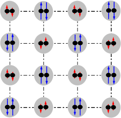
Figure 1: (Color online) The picture of the staggered spin-quadrupole long-range ordered state with the order parameter $(-1)^{i}\langle n_{i}^{4}\rangle$ on a two-dimensional square lattice, where each site is occupied by a spin singlet state. The long blue arrow and short red arrow denote a fermion with $S^{z}=\pm\frac{3}{2}$ and $S^{z}=\pm\frac{1}{2}$, respectively.

Another interesting physics in the spin-quadrupole ordering state is the non-abelian Berry phase. Since the four-component SO(5) spinor forms a seven-dimensional sphere $S^{7}$, the adiabatic rotation of the fermionic quasiparticle in spin-quadrupole ordering state defines the second Hopf map

$$S^{7}\rightarrow S^{4},$$ (14)

which enables an interesting non-abelian SU(2) gauge connection of the so-called Wilczek-Zee holonomy Wilczek-1984 ; Demler-1999 . Mathematically, it is understood that $S^{7}$ is an SU(2) bundle over $S^{4}$ sphere. Therefore, the topological structure of the spin-quadrupole ordering state is described by the second Hopf map and the second Chern number. As the fermionic quasiparticle spectrum is two-fold degenerate, once we perform an adiabatic circuit rotation of the superspin vector $n_{i}^{a}$, the spinor state can be a linear combination of the two degenerate low energy states, which is related to the original state by a $2\times 2$ unitary transformation matrix. Actually, the SU(2) non-abelian Berry phase is also present in the quintet pairing state Chern-2004 and plays a key role in the entanglement generation between the fermionic quasiparticles and the half-quantum vortex CWu-Hu-2005 .

IV Degenerate antiferromagnetic spin-dipole / spin-octupole ordering state

IV.1 Saddle point approximation

Next we will consider the case for $c_{2}<0$, where a spin quintet state is formed by two spin-$\frac{3}{2}$ fermions on each lattice site with total spin $S=2$. Applying the SU(4) Fierz identity

$$\sum_{1\leq a<b\leq 5}(L_{i}^{ab})^{2}+\sum_{1\leq a\leq 5}(n_{i}^{a})^{2}+\frac{5}{4}(N_{i}-2)^{2}=5,$$ (15)

to the interactions of the model Hamiltonian, we can rewrite the generalized one-band Hubbard model as

$$H = -t\sum_{\langle ij\rangle,\alpha}(\psi_{i\alpha}^{{\dagger}}\psi_{j\alpha}+\text{H.c.})+\frac{3c_{2}}{4}\sum_{i,1\leq a<b\leq 5}(L_{i}^{ab})^{2}$$ (16)

$$+\frac{c_{0}}{2}\sum_{i}(N_{i}-2)^{2}-\mu\sum_{i}N_{i},$$

where the chemical potential $\mu$ is set zero at half filling. As far as the Mott insulating phase is concerned, the particle number fluctuations can be neglected safely, and the spin-dipole and spin-octupole fluctuations become dominant when $c_{2}<0$.

Formally, the partition function is written as a path integral

$$Z=\int\mathcal{D}\psi^{{\dagger}}\mathcal{D}\psi\exp\left[-\int_{0}^{\beta}L\left(\tau\right)d\tau\right],$$ (17)

where $\beta=\frac{1}{k_{B}T}$ and the Lagrangian is given by $L=\sum_{i,\alpha}\psi_{i\alpha}^{{\dagger}}\partial_{\tau}\psi_{i\alpha}+H$. In the following we denote $U\equiv-\frac{3}{4}c_{2}$ for simplicity and a Hubbard-Stratonovich transformation is performed

$$\exp\left[U\int_{0}^{\beta}d\tau\sum_{i,a<b}(L_{i}^{ab})^{2}\right]$$

$$= \int\mathcal{D}\varphi\exp\left[\int_{0}^{\beta}d\tau\sum_{i,a<b}\left(\sqrt{2U}\varphi_{i}^{ab}L_{i}^{ab}-\frac{1}{2}(\varphi_{i}^{ab})^{2}\right)\right],$$

where a ten-component order parameter field $\varphi$ is introduced. By integrating out the fermion fields, an effective action is obtained as

$$S_{\text{eff}}=\int_{0}^{\beta}d\tau\sum_{i,a<b}\frac{1}{2}(\varphi_{i}^{ab})^{2}-\text{Tr}\ln\left[\partial_{\tau}+\mathbf{M}\right],$$ (18)

where the trace is taken over the spinor space, the spatial and imaginary time coordinates. The matrix element of $\mathbf{M}$ and Green’s function (GF) of the fermions satisfy

$$\langle\mathbf{r}_{i},\tau,\alpha|\mathbf{M}|\mathbf{r}_{j},\tau^{\prime},\beta\rangle = -2t\delta_{\tau\tau^{\prime}}\delta_{i,j+\delta}\delta_{\alpha\beta}$$

$$+\sqrt{\frac{U}{2}}\delta_{\tau\tau^{\prime}}\delta_{ij}\sum_{a<b}\varphi_{i}^{ab}\Gamma_{\alpha\beta}^{ab},$$

$$G_{\alpha\beta}(\mathbf{r}_{i},\tau;\mathbf{r}_{j},\tau^{\prime}) = \langle\mathbf{r}_{i},\tau,\alpha|\frac{-1}{\partial_{\tau}+\mathbf{M}}|\mathbf{r}_{j},\tau^{\prime},\beta\rangle.$$ (19)

So far no approximations have been made. Once we perform a loop expansion on the effective action with respect to $\varphi$, the instability owing the negative coefficient of the quadratic term in $\varphi$ is dominated by the so-called Fermi surface instability, which is similar to the well-known antiferromagnetic instability in half filled Hubbard model Nagaosa .

In order to determine the long range order of Mott insulator, we first consider the saddle point solution of the effective action. Differentiating $S_{\text{eff}}$ with respect to $\varphi_{i}^{ab}\left(\tau\right)$, we obtain the equation

$$\varphi_{i}^{ab}\left(\tau\right)=-\sqrt{\frac{U}{2}}\underset{\alpha\beta}{\sum}G_{\alpha\beta}(\mathbf{r}_{i},\tau;\mathbf{r}_{i},\tau)\Gamma_{\beta\alpha}^{ab}.$$ (20)

Then it is expected that the ground state is in a staggered phase of the SO(5) adjoint order parameter, namely, a staggered degenerate spin-dipole /spin-octupole ordering phase with a static order parameter field $\varphi_{i}^{ab}\left(\tau\right)\rightarrow|\varphi|e^{i\mathbf{Q}\cdot\mathbf{r}_{i}}d^{ab}$, where $\mathbf{Q}=(\pi,\pi)$ corresponds to the nesting vector in a two-dimensional square lattice, and $d^{ab}$ is the symmetry breaking direction. The degeneracy of spin-dipole and spin-octupole order is protected by the exact SO(5) symmetry of the Hamiltonian, which implies the spin-dipole operators can be rotated to spin-octupole operators and vice versa. Thus, this degeneracy is robust against quantum and thermal fluctuations. However, an anisotropy, such as lattice potential, will pin down a special choice of the ground state. Actually, the effective action at the saddle point becomes

$$S^{(0)} = \sum_{\mathbf{k},i\mathbf{\omega}_{n}}\left\{\psi_{\mathbf{k}}^{{\dagger}}(i\mathbf{\omega}_{n})\left(-i\mathbf{\omega}_{n}+\varepsilon_{\mathbf{k}}\right)\psi_{\mathbf{k}}(i\mathbf{\omega}_{n})+\frac{1}{2}\beta N|\varphi|^{2}\right.$$ (21)

$$\left.+\sqrt{\frac{U}{2}}|\varphi|\sum_{a<b}\psi_{\mathbf{k}}^{{\dagger}}(i\mathbf{\omega}_{n})d^{ab}\Gamma^{ab}\psi_{\mathbf{k}-\mathbf{Q}}(i\mathbf{\omega}_{n})\right\},$$

where the fermion dispersion relation is $\varepsilon_{\mathbf{k}}=-2t(\cos k_{x}+$ $\cos k_{y})$, and $\mathbf{\omega}_{n}$ is the fermionic Matsubara frequency. The fermion GF has to be defined as $G_{\alpha\beta}\left(\mathbf{k},\mathbf{k}^{\prime};\tau\right)=-\langle T_{\tau}\psi_{\mathbf{k}\alpha}(\tau)\psi_{-\mathbf{k}^{\prime}\beta}^{{\dagger}}(0)\rangle$, which has non-zero off-diagonal terms in momentum space due to the umklapp processes with respect to $\mathbf{Q}$. At the saddle point, the fermion single particle GF is given by

$$G_{\alpha\beta}\left(\mathbf{k},-\mathbf{k}^{\prime};i\omega_{n}\right)$$ (22)

$$= \frac{\left(i\omega_{n}+\varepsilon_{\mathbf{k}}\right)\delta_{\alpha\beta}\delta_{\mathbf{kk}^{\prime}}+\sqrt{\frac{U}{2}}|\varphi|\sum_{a<b}d^{ab}\Gamma_{\alpha\beta}^{ab}\delta_{\mathbf{k}^{\prime},\mathbf{k}-\mathbf{Q}}}{(i\omega_{n})^{2}-E_{\mathbf{k}}^{2}},$$

where GF poles determine the fermionic quasiparticle spectrum $E_{\mathbf{k}}=\pm\sqrt{\varepsilon_{\mathbf{k}}^{2}+\frac{U}{2}|\varphi|^{2}}$. At half filling, the upper band is empty while the lower band is completely filled. Thus an energy gap $\Delta=2\sqrt{\frac{U}{2}}|\varphi|$ opens up in the single particle spectrum. At $T=0$K, the gap equation is given by

$$\frac{1}{U}=\frac{1}{N}\sum_{\mathbf{k}}\frac{1}{E_{\mathbf{k}}}.$$ (23)

In the limit of $U\ll t$, it gives rise to $\Delta\simeq 2te^{-\pi\sqrt{2t/U}}$, which implies the Fermi surface is fully gapped for arbitrary small but finite $U$. For $U\gg t$, we have $\Delta\simeq 2U$, i.e., a large Mott gap.

We have shown two typical configurations of this long-range ordering phase in Fig. 2, and the corresponding order parameters are denoted by $(-1)^{i}\langle L_{i}^{15}\rangle\neq 0$ and $(-1)^{i}\langle L_{i}^{23}\rangle\neq 0$, respectively. More explicitly, $L_{i}^{15}$ and $L_{i}^{23}$ are expressed as

$$2L_{i}^{15} = \psi_{i,\frac{3}{2}}^{\dagger}\psi_{i,\frac{3}{2}}+\psi_{i,\frac{1}{2}}^{\dagger}\psi_{i,\frac{1}{2}}-\psi_{i,-\frac{1}{2}}^{\dagger}\psi_{i,-\frac{1}{2}}-\psi_{i,-\frac{3}{2}}^{\dagger}\psi_{i,-\frac{3}{2}},$$

$$2L_{i}^{23} = \psi_{i,\frac{1}{2}}^{\dagger}\psi_{i,\frac{1}{2}}+\psi_{i,-\frac{3}{2}}^{\dagger}\psi_{i,-\frac{3}{2}}-\psi_{i,\frac{3}{2}}^{\dagger}\psi_{i,\frac{3}{2}}-\psi_{i,-\frac{1}{2}}^{\dagger}\psi_{i,-\frac{1}{2}},$$

corresponding to two different patterns of total $S^{z}=\pm 2$ and $S^{z}=\pm 1$ of two atoms in the site-quintet state, respectively. Actually, both configurations display the coexistence of antiferromagnet spin-dipole and staggered spin-octupole ordering with breaking the spin SU(2) and time reversal symmetries.

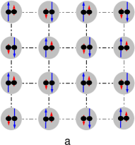
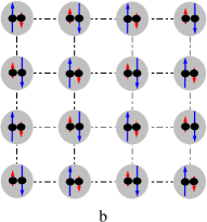
Figure 2: (Color online) The picture of the long range ordered state with the order parameter $(-1)^{i}\langle L_{i}^{15}\rangle$ (a) and $(-1)^{i}\langle L_{i}^{23}\rangle$ (b) on a two-dimensional square lattice, where each site is occupied by a spin quintet state.

To simplify the following discussions, we assume the order parameter is fixed by $(-1)^{i}\langle L_{i}^{15}\rangle\neq 0$. Along with the order parameter $L_{i}^{15}$ acquires non-zero vacuum expectation value, the SO(5) generators $L_{i}^{15}$, $L_{i}^{23}$, $L_{i}^{24}$ and $L_{i}^{34}$ still keep the ordering state invariant, where the latter three SO(5) generators form an SU(2) subgroup. Therefore, the Goldstone manifold is SO(5)/[SU(2)$\times$U(1)]=CP³, which is a six-dimensional complex projective space. According to the Goldstone theorem, there will be six branches of Goldstone bosons induced by the spontaneous symmetry breaking.

The topological aspects on the degenerate spin-dipole/spin-octupole ordering phase are also interesting. Mathematically, a seven-dimensional sphere $S^{7}$ can be viewed as a U(1) bundle over CP³, which is the Goldstone manifold in the current case. Because the four-component SO(5) spinor lives on $S^{7}$, the adiabatic circuit rotation of the fermionic quasiparticles in the degenerate spin-dipole with spin-octupole ordering state defines a U(1) gauge connection. Although the fermionic quasiparticle spectrum is also two-fold degenerate, once an adiabatic circuit rotation of the order parameter $L_{i}^{ab}$ is performed, only an additional U(1) phase factor can be generated in the resulting spinor state, instead of linear combination of the two degenerate states due to the abelian nature of the U(1) Berry phase Berry-1984 . Therefore, unlike the spin-quadrupole ordering state, the topological structure of the degenerate spin-dipole /spin-octupole ordering state is characterized by the U(1) abelian Berry phase  and the first Chern number.

IV.2 Gaussian fluctuations

To further study the collective excitations, we consider Gaussian fluctuations around the saddle point solution, $\varphi=\varphi_{c}+\delta\varphi$. Then the effective action $S_{\text{eff}}$ can be expanded as $S_{\text{eff}}=\sum_{n=0}^{\infty}S^{(n)}(\varphi_{c},\delta\varphi)$ from

$$\text{Tr}\ln\left[\partial_{\tau}+\mathbf{M}\right]=\text{Tr}\ln(-\mathbf{G}^{-1})-\sum_{n}\frac{1}{n}\text{Tr}(\mathbf{GV})^{n},$$ (24)

where $\mathbf{G}$ represents the fermion GF at the saddle point and the matrix element of $\mathbf{V}$ is given by

$$\langle\mathbf{r}_{i},\tau,\alpha|\mathbf{V}|\mathbf{r}_{j},\tau^{\prime},\beta\rangle=\delta_{\tau\tau^{\prime}}\delta_{ij}\sqrt{\frac{U}{2}}\sum_{a<b}\delta\varphi_{i}^{ab}\left(\tau\right)\Gamma_{\alpha\beta}^{ab}.$$ (25)

Since $\mathbf{V}$ only contains a linear term in $\delta\varphi$, the above procedure is indeed an expansion in the spin-dipole and spin-octupole fluctuations. The first order term in $\delta\varphi$ vanishes due to the saddle point equation. The Fourier transformation of $\delta\varphi_{i}^{ab}\left(\tau\right)$ is defined by

$$\delta\varphi_{i}^{ab}\left(\tau\right)=\frac{1}{\sqrt{\beta N}}\sum_{\mathbf{p},i\omega_{l}}\delta\varphi_{\mathbf{p}}^{ab}\left(i\omega_{l}\right)e^{i\mathbf{p}\cdot\mathbf{r}_{i}-i\omega_{l}\tau},$$ (26)

where $\omega_{l}$ are bosonic Matsubara frequencies. After some straightforward algebra, up to the second order expansion in the fluctuation field $\delta\varphi$, we arrive at

$$S^{(2)} = \sum_{\mathbf{p},i\omega_{l}}\left\{K_{0}(\mathbf{p},i\omega_{l})\Phi_{-\mathbf{p}}^{T}(-i\omega_{l})\Phi_{\mathbf{p}}(i\omega_{l})\right.$$ (27)

$$+\sum_{a=2,3,4}K_{1}(\mathbf{p},i\omega_{l})[\delta\varphi_{-\mathbf{p}}^{1a}\left(-i\omega_{l}\right)\delta\varphi_{\mathbf{p}}^{1a}\left(i\omega_{l}\right)+\delta\varphi_{-\mathbf{p}}^{a5}\left(-i\omega_{l}\right)\delta\varphi_{\mathbf{p}}^{a5}\left(i\omega_{l}\right)]$$

$$+\sum_{a=2,3,4}\left.K_{2}(\mathbf{p},i\omega_{l})[\delta\varphi_{-\mathbf{p}-\mathbf{Q}}^{1a}\left(-i\omega_{l}\right)\delta\varphi_{\mathbf{p}}^{a5}\left(i\omega_{l}\right)-\delta\varphi_{-\mathbf{p}-\mathbf{Q}}^{a5}\left(-i\omega_{l}\right)\delta\varphi_{\mathbf{p}}^{1a}\left(i\omega_{l}\right)]\right\},$$

where $\Phi_{i}=(\delta\varphi_{i}^{15},\delta\varphi_{i}^{23},\delta\varphi_{i}^{24},\delta\varphi_{i}^{34})^{T}$ is a Nambu spinor and the kernel functions are given by

$$K_{0}(\mathbf{p},i\omega_{l})=\frac{1}{2}-\frac{U}{\beta N}\sum_{\mathbf{k},i\mathbf{\omega}_{n}}\frac{\omega_{n}\left(\omega_{n}+\omega_{l}\right)-\varepsilon_{\mathbf{k}}\varepsilon_{\mathbf{k+p}}-\frac{\Delta^{2}}{4}}{(\omega_{n}^{2}+E_{\mathbf{k}}^{2})\left[\left(\omega_{n}+\omega_{l}\right)^{2}+E_{\mathbf{k}+\mathbf{p}}^{2}\right]},$$ (28)

$$K_{1}(\mathbf{p},i\omega_{l})=\frac{1}{2}-\frac{U}{\beta N}\sum_{\mathbf{k},i\mathbf{\omega}_{n}}\frac{\omega_{n}\left(\omega_{n}+\omega_{l}\right)-\varepsilon_{\mathbf{k}}\varepsilon_{\mathbf{k+p}}+\frac{\Delta^{2}}{4}}{(\omega_{n}^{2}+E_{\mathbf{k}}^{2})\left[\left(\omega_{n}+\omega_{l}\right)^{2}+E_{\mathbf{k}+\mathbf{p}}^{2}\right]},$$ (29)

$$K_{2}(\mathbf{p},i\omega_{l})=\frac{U\Delta}{2\beta N}\sum_{\mathbf{k},i\mathbf{\omega}_{n}}\frac{\omega_{l}}{(\omega_{n}^{2}+E_{\mathbf{k}}^{2})\left[\left(\omega_{n}+\omega_{l}\right)^{2}+E_{\mathbf{k}+\mathbf{p}}^{2}\right]}.$$ (30)

In the low energy limit $i\omega_{l}\rightarrow 0$, for the momentum transfer $\mathbf{p}=\mathbf{Q}$, $K_{0}\left(\mathbf{Q},0\right)>0$ and $K_{1}\left(\mathbf{Q},0\right)=K_{2}\left(\mathbf{Q},0\right)=0$ following from the gap equation. Therefore, the collective excitation modes in the first term of Eq.(27) is gapped, and the remaining terms describe the Goldstone modes related to the symmetry breaking. From Eq.(27), we notice that the couplings between the fluctuating Goldstone fields are in a twin form as $\delta\varphi^{12}\delta\varphi^{25}$, $\delta\varphi^{13}\delta\varphi^{35}$ and $\delta\varphi^{14}\delta\varphi^{45}$. As we discussed, the resulting effective action enjoys a residual SU(2)$\times$U(1) symmetry and the coupling between the Goldstone fields are allowed.

In order to evaluate the low energy behavior of the Goldstone bosons, we perform the summation over the Matsubara frequency in the kernel functions of $K_{1}$, $K_{2}$ and analytical continuation $i\omega_{l}\rightarrow\omega+i0^{+}$. When the long wavelength and low energy limit are considered at $T=0$K, the kernel functions are expanded to the leading order in $\mathbf{q}$ and $\omega$ as

$$K_{1}(\mathbf{Q}+\mathbf{q},\omega) \approx a\mathbf{q}^{2}-b\omega^{2},\text{ }K_{1}(\mathbf{q},\omega)\approx d,$$

$$K_{2}(\mathbf{Q}+\mathbf{q},\omega) = K_{2}(\mathbf{q},\omega)\approx c\omega,$$ (31)

where the coefficients are given by

$$a=\int_{-\pi}^{\pi}\frac{d^{2}\mathbf{k}}{(2\pi)^{2}}\frac{Ut^{2}\sin^{2}k_{x}}{2E_{\mathbf{k}}^{3}},\text{ }b=\int_{-\pi}^{\pi}\frac{d^{2}\mathbf{k}}{(2\pi)^{2}}\frac{U}{8E_{\mathbf{k}}^{3}},c=-\int_{-\pi}^{\pi}\frac{d^{2}\mathbf{k}}{(2\pi)^{2}}\frac{iU\Delta}{8E_{\mathbf{k}}^{3}},\text{ }d=\int_{-\pi}^{\pi}\frac{d^{2}\mathbf{k}}{(2\pi)^{2}}\frac{U\varepsilon_{\mathbf{k}}^{2}}{2E_{\mathbf{k}}^{3}}.$$ (32)

Thus, the effective action describing the Goldstone bosons is given by

$$S_{\text{GB}}=\int\frac{d\mathbf{q}d\omega}{(2\pi)^{3}}\sum_{a=2,3,4}\left(\begin{array}[]{c}\delta\varphi_{-\mathbf{q}-\mathbf{Q}}^{1a}\left(-\omega\right)\\ \delta\varphi_{-\mathbf{q}}^{1a}\left(-\omega\right)\\ \delta\varphi_{-\mathbf{q}-\mathbf{Q}}^{a5}\left(-\omega\right)\\ \delta\varphi_{-\mathbf{q}}^{a5}\left(-\omega\right)\end{array}\right)^{T}\left(\begin{array}[]{cccc}a\mathbf{q}^{2}-b\omega^{2}&0&0&c\omega\\ 0&d&c\omega&0\\ 0&-c\omega&a\mathbf{q}^{2}-b\omega^{2}&0\\ -c\omega&0&0&d\end{array}\right)\left(\begin{array}[]{c}\delta\varphi_{\mathbf{q}+\mathbf{Q}}^{1a}\left(\omega\right)\\ \delta\varphi_{\mathbf{q}}^{1a}\left(\omega\right)\\ \delta\varphi_{\mathbf{q}+\mathbf{Q}}^{a5}\left(\omega\right)\\ \delta\varphi_{\mathbf{q}}^{a5}\left(\omega\right)\end{array}\right).$$ (33)

Then the dispersion relation of the Goldstone bosons is determined by the pole of the collective mode correlation functions, giving rise to $\omega=v|\mathbf{q}|$, a linear dispersion with the density wave velocity

$$v=\sqrt{\frac{ad}{bd-c^{2}}}.$$ (34)

The corresponding numerical results are displayed in Fig. 3.

Figure 3: The degenerate spin-dipole/spin-octupole density wave velocity $v$ (dotted line) is compared with the spin-quadrupole wave velocity $v_{\text{Q}}$ (solid line).

In the small $U$ limit, the density wave velocity is approximated by $v\approx 2t(2U/t)^{1/4}/\sqrt{\pi}$, while in the large $U$ limit, it is given by $v\approx 2\sqrt{2}t^{2}/U$. Due to the presence of the coupled vibrations of the transverse modes, the wave velocity is suppressed in the strong coupling limit, in a sharp contrast to the velocity of the spin-quadrupole density waves. These properties can be understood on the basis of the symmetry considerations. The transverse mode couplings in spin-quadrupole density waves are absent because the SO(4) invariance of the effective action under the Gaussian fluctuations does not allow such couplings. However, the residual SU(2)$\times$U(1) symmetry does allow coupled vibrations of the Goldstone modes, which is analogous to the transverse spin wave mixing in half filled spin-$\frac{1}{2}$ Hubbard model.

V Algebraic spin liquid state

In the previous sections, we have established the spin-ordered Mott insulating phases of spin-$\frac{3}{2}$ fermions in various limits. Near the special SU(4) point, the energies of the ordering states are very close to each other. Since these two competing ordering ground states exhibit quite different symmetry properties, low energy excitations and topological characterizations, a continuous quantum phase transition from one to another is almost impossible. Therefore a nontrivial quantum critical state may emerge around the SU(4) symmetric point.

V.1 SU(4) symmetric point

Let us first consider the SU(4) point ($c_{2}=0$). In this case, the generalized one-band Hubbard model at half filling is reduced to the SU(4) Hubbard model:

$$H=-t\sum_{\langle ij\rangle,\alpha}(\psi_{i\alpha}^{{\dagger}}\psi_{j\alpha}+\text{H.c.})+\frac{c_{0}}{2}\sum_{i}(N_{i}-2)^{2}.$$ (35)

When the strong coupling limit ($c_{0}\gg t$) is considered, the effective exchange model can be derived by a second-order perturbation theory, which reads

$$H_{\text{eff}}=J\sum_{\langle ij\rangle}(\sum_{1\leq a<b\leq 5}L_{i}^{ab}L_{j}^{ab}+\sum_{1\leq a\leq 5}n_{i}^{a}n_{j}^{a}),$$ (36)

where the coupling constant $J\sim t^{2}/c_{0}$. When we introduce a spinon representation in terms of four component fermions, the operators $n_{i}^{a}$ and $L_{i}^{ab}$ can be expressed as

$$n_{i}^{a} = \frac{1}{2}\sum_{\alpha\beta}f_{i\alpha}^{{\dagger}}\Gamma_{\alpha\beta}^{a}f_{i\beta}\;(1\leq a\leq 5),$$

$$L_{i}^{ab} = -\frac{1}{2}\sum_{\alpha\beta}f_{i\alpha}^{{\dagger}}\Gamma_{\alpha\beta}^{ab}f_{i\beta}\;(1\leq a<b\leq 5),$$ (37)

with a local constraint $\sum_{\alpha}f_{i\alpha}^{{\dagger}}f_{i\alpha}=2$. The effective model Hamiltonian can thus be written as

$$H_{\text{eff}}=-J\sum_{\langle ij\rangle,\alpha\beta}f_{i\alpha}^{{\dagger}}f_{j\alpha}f_{j\beta}^{{\dagger}}f_{i\beta}.$$ (38)

This is nothing but the SU(4) quantum antiferromagnetic Heisenberg model, which was studied in the large-$N$ limit on a square lattice by Affleck and Marston Affleck-1988 . Formally, we can express the partition function as a path integral

$$Z=\int\mathcal{D}f^{{\dagger}}\mathcal{D}f\mathcal{D}\lambda\exp\left[-\int_{0}^{\beta}L_{\text{eff}}(\tau)d\tau\right],$$ (39)

where the effective Lagrangian is given by

$$L_{\text{eff}}=\sum_{i,\alpha}f_{i\alpha}^{{\dagger}}\partial_{\tau}f_{i\alpha}+H_{\text{eff}}+\sum_{i}\lambda_{i}\left(\sum_{\alpha}f_{i\alpha}^{{\dagger}}f_{i\alpha}-2\right),$$ (40)

and the Lagrange multiplier field $\lambda_{i}$ is introduced to impose the local constraint. Then the interaction part can be decoupled via a valence bond auxiliary field

$$\exp\left[\int_{0}^{\beta}d\tau\sum_{\langle ij\rangle,\alpha\beta}f_{i\alpha}^{{\dagger}}f_{j\alpha}f_{j\beta}^{{\dagger}}f_{i\beta}\right]$$ (41)

$$= \int\mathcal{D}\chi e^{\int_{0}^{\beta}d\tau\left[\sum_{\langle ij\rangle,\alpha}(f_{i\alpha}^{{\dagger}}f_{j\alpha}\chi_{ji}+\text{c.c.})-\sum_{\langle ij\rangle}|\chi_{ij}|^{2}\right]},$$

where $\chi_{ij}=\chi_{ji}^{\ast}=|\chi_{ij}|e^{-ia_{ij}}$ and $a_{ij}$ is a phase field. Under the gauge transformation $a_{ij}\rightarrow a_{ij}+\theta_{i}-\theta_{j}$, $f_{i}\rightarrow f_{i}e^{i\theta_{i}}$, the effective action is invariant, because $\partial_{\tau}\theta_{i}$ term can be absorbed in the Lagrange multiplier. The gauge invariance thus gives rise to a U(1) gauge field, which is also related to the local constraint. By gauge fixing, $\chi_{ij}$ can be chosen to be real, and a saddle point approximation leads to the $\pi$-flux state with

$$\chi_{i,i+x}=-\chi(-1)^{i_{y}},\text{ }\chi_{i,i+y}=\chi,\text{ }$$ (42)

and the Lagrangian multiplier is fixed by the particle-hole symmetry at $\lambda_{i}=0$. Although the above mean-field ansatz breaks the lattice translation symmetry, it can be restored when projecting the mean-field state onto the physical Hilbert space with two spinons per site. Then the effective model can be written as

$$H_{\pi\text{F}} = 2JN\chi^{2}-J\chi\sum_{i\alpha}(f_{i\alpha}^{{\dagger}}f_{i+y,\alpha}+f_{i\alpha}^{{\dagger}}f_{i-y,\alpha}$$ (43)

$$-(-1)^{i_{y}}f_{i\alpha}^{{\dagger}}f_{i-x,\alpha}-(-1)^{i_{y}}f_{i\alpha}^{{\dagger}}f_{i+x,\alpha}),$$

which is quadratic in spinon operators and is easily diagonalized. The spinon excitation spectrum is obtained by $\epsilon_{\mathbf{k}}^{\pm}=\pm 2J\chi\sqrt{\cos^{2}k_{x}+\cos^{2}k_{y}}$ with four gapless nodes at $k_{x}=\pm\frac{\pi}{2}$ and $k_{y}=\pm\frac{\pi}{2}$. The ground state energy per site is determined by filling the negative spinon bands:

$$\epsilon_{\pi\text{F}}=4\int_{-\pi}^{\pi}\frac{dk_{x}}{2\pi}\int_{-\frac{\pi}{2}}^{\frac{\pi}{2}}\frac{dk_{y}}{2\pi}\epsilon_{\mathbf{k}}^{-}+2J\chi^{2},$$ (44)

where the minimum energy is attained at $\chi=0.958091$. When taking into account the nodal SU(2) symmetry in the low energy limit, the $\pi$-flux state gains an emergent SU(8) symmetry Hermele-2005 .

In fact, the low energy effective theory of the SU(4) $\pi$-flux states should be described by a fluctuating massless U(1) gauge field minimally coupled to the Dirac spinons. This is different from the $\pi$-flux state with a gapless SU(2) gauge field in the spin-1/2 quantum Heisenberg antiferromagnets. However, the SU(4) $\pi$-flux state resembles the SU(2) staggered flux state. Recently, Hermele et al. argued that if the spin index is generalized to $N$, the problem of $2N$ two-component Dirac fermions coupled to a compact U(1) gauge field is deconfined for sufficient large $N$ Hermele-2004 . Furthermore, Assaad has performed quantum Monte Carlo simulations of the SU($N$) antiferromagnetic Heisenberg model on the square lattice and found that the optimal ground state for $N=4$ is a $\pi$-flux state with gapless spinon excitation and spin algebraic correlations Assaad-2005 . The lattice translational and spin rotational symmetries are preserved in such a $\pi$-flux state. Thus, a system of interacting spin-$\frac{3}{2}$ fermionic ultracold atoms at half-filling in a two-dimensional square optical lattice is a possible experimental realization to observe this interesting algebraic spin liquid state. The equal-time spin-quadrupole correlations and the SO(5) adjoint operator correlation functions display the same power-law behavior due to the SU(4) symmetry

$$(-1)^{(i_{x}+i_{y})}\left\langle n_{i}^{a}n_{0}^{a}\right\rangle=(-1)^{(i_{x}+i_{y})}\left\langle L_{i}^{ab}L_{0}^{ab}\right\rangle\sim\frac{1}{|\mathbf{r}_{i}|^{\eta}},$$ (45)

which in principle can be measured by spatial noise correlation experiments Altman-2004 ; Folling-2005 . In the mean field description, the correlation functions in the $\pi$-flux state decay as $1/|\mathbf{r}|^{4}$, because the spinons are effectively described by (2+1) dimensional relativistic free Dirac fermions at low energy regime. However, the gauge fluctuations are expected to enhance the correlations functions as shown in the quantum Monte Carlo results ($1/|\mathbf{r}|^{1.12}$) Assaad-2005 and the calculations including the gauge fluctuations in a large-$N$ approximation Rantner-2001 .

V.2 Effective model and the phase diagram

According to the Landau’s continuous phase transition theory, two phases with incompatible symmetries can not be connected by a continuous phase transition Senthil-2004 . In the previous section, our mean field theory have shown that the quantum critical $\pi$-flux state separates two insulating long-range ordered states, which are characterized by different symmetries, order parameters, and topological characterizations. However, we can not rule out the possibility that the quantum critical $\pi$-flux state actually controls a region in the parameter space. Moreover, our saddle point approaches to the generalized Hubbard model have neglected the particle number fluctuations, however, such particle number fluctuations may melt the assumed spin ordering at small but finite $c_{2}$ and stabilize the algebraic spin liquid state. Our system provides such a chance to study the quantum critical phase within the Landau’s paradigm.

Let us start from the effective Hamiltonian in the strong coupling limit CWu-2006

$$H_{\text{eff}}=J_{1}\sum_{\langle ij\rangle,a<b}L_{i}^{ab}L_{j}^{ab}+J_{2}\sum_{\langle ij\rangle,a}n_{i}^{a}n_{j}^{a}+J_{3}\sum_{i,a<b}(L_{i}^{ab})^{2},$$ (46)

where $J_{3}\propto c_{2}$. At the SU(4) point, $J_{3}=0$ and $J_{1}=J_{2}=4t^{2}/c_{0}$, the effective model is reduced to the previous SU(4) Heisenberg antiferromagnetic spin model. In the spin-quadrupole ordering phase, we should have $J_{2}\gg J_{1}>0$ and $J_{3}>0$, the first term can be neglected, and the effective model Hamiltonian becomes an SO(5) quantum rotor model. However, in degenerate antiferromagnetic spin-dipole/spin-octupole ordering phase, we should have $J_{1}\gg J_{2}>0$ and $J_{3}<0$, the latter two terms can be neglected, and the effective model is reduced to an SO(5) Heisenberg antiferromagnetic spin model. Thus, this effective model Hamiltonian well describes the basic physics of the system from the strong coupling limit. In this effective model, the virtue tunnelling processes of atoms between lattice sites have been taken into account, and the various spin ordering formation can be regarded as possible instabilities of algebraic spin liquid state.

V.2.1 Staggered spin-quadrupole ordering state

Since $J_{2}>J_{1}$ and $J_{3}>0$, we have to find relevant interactions for instability of the $\pi$-flux state to spin-quadrupole fluctuations. Again we use the fermionic spinon representations and the effective Hamiltonian can be expressed as

$$H_{\text{eff}} = -J_{1}\sum_{\langle ij\rangle,\alpha\beta}f_{i\alpha}^{{\dagger}}f_{j\alpha}f_{j\beta}^{{\dagger}}f_{i\beta}+{}J_{-}\sum_{\langle ij\rangle,a}n_{i}^{a}n_{j}^{a}$$ (47)

$$-J_{3}\sum_{i,a}(n_{i}^{a})^{2},$$

where $J_{-}=J_{2}-J_{1}$ and spinon number satisfy the constraint $\sum_{\alpha}f_{i\alpha}^{{\dagger}}f_{i\alpha}=2$. Since $J_{-}>0$ and $J_{3}>0$, the first term is decoupled according to the valence bond order parameters in the $\pi$-flux state as (42) and the latter two terms are treated in a mean field approximation. The following staggered spin-quadrupole order parameter is introduced

$$(-1)^{i}\left\langle n_{i}^{4}\right\rangle=\Delta,\text{ }(-1)^{i}\left\langle n_{i}^{a}\right\rangle=0\text{ }(a\neq 4)\text{.}$$ (48)

Then, the mean field Hamiltonian can be obtained as

$$H_{\text{MF}} = 2J_{1}\chi\sum_{\mathbf{k},\alpha}\left[\left(\cos k_{x}\right)f_{\mathbf{k}\alpha}^{{\dagger}}f_{\mathbf{k}-\pi\hat{k}_{y},\alpha}-\left(\cos k_{y}\right)f_{\mathbf{k}\alpha}^{{\dagger}}f_{\mathbf{k}\alpha}\right]$$ (49)

$$-(2{}J_{-}+J_{3})\Delta\sum_{\mathbf{k},\alpha\beta}f_{\mathbf{k}\alpha}^{{\dagger}}\Gamma_{\alpha\beta}^{4}f_{\mathbf{k}-\mathbf{Q},\beta}$$

$$+2J_{1}\chi^{2}N+(2{}J_{-}+J_{3})\Delta^{2}N,$$

which can be easily diagonalized. The spinon quasiparticle spectrum is thus derived as

$$E_{\mathbf{k}}^{\pm}=\pm\sqrt{4J_{1}^{2}\chi^{2}(\cos^{2}k_{x}+\cos^{2}k_{y})+(2{}J_{-}+J_{3})^{2}\Delta^{2}},$$ (50)

where an energy gap is induced by the formation of the long range spin-quadrupole ordering. By minimizing the ground state energy, a set of self-consistent equations determining the order parameters $\chi$ and $\Delta$ are deduced to

$$\int_{-\frac{\pi}{2}}^{\frac{\pi}{2}}\frac{dk_{x}dk_{y}}{(2\pi)^{2}}\frac{\left(\cos^{2}k_{x}+\cos^{2}k_{y}\right)}{E_{\mathbf{k}}^{+}} = \frac{1}{8J_{1}},$$

$$\int_{-\frac{\pi}{2}}^{\frac{\pi}{2}}\frac{dk_{x}dk_{y}}{(2\pi)^{2}}\frac{4(2J_{-}+J_{3})}{E_{\mathbf{k}}^{+}} = 1.$$ (51)

From these equations, we can easily find the critical condition, i.e. the boundary between the spin-quadrupole ordering and the $\pi$-flux state. By setting $\Delta=0$, we find the phase boundary as

$$\frac{J_{3}}{J_{2}}\approx-3.49\frac{J_{-}}{J_{2}}+1.49.$$ (52)

V.2.2 Degenerate antiferromagnetic spin-dipole/spin-octupole ordering state

Next we turn to the parameter regime in which spin-dipole and spin-octupole fluctuations are dominant. To investigate the long-range order formation, the effective Hamiltonian can be rewritten as

$$H_{\text{eff}} = -J_{2}\sum_{\langle ij\rangle,\alpha\beta}f_{i\alpha}^{{\dagger}}f_{j\alpha}f_{j\beta}^{{\dagger}}f_{i\beta}-{}J_{-}\sum_{\langle ij\rangle,a<b}L_{i}^{ab}L_{j}^{ab}$$ (53)

$$+J_{3}\sum_{i,a<b}(L_{i}^{ab})^{2}.$$

Since $J_{-}<0$ and $J_{3}<0$, the valence bond order parameter as the $\pi$-flux state as (42) can be chosen for the first term and a mean field approximation can be made for the last two terms. Then the degenerate antiferromagnetic spin-dipole/spin-octupole order parameter is introduced by

$$(-1)^{i}\left\langle L_{i}^{15}\right\rangle=\Delta,\text{ }(-1)^{i}\left\langle L_{i}^{ab}\right\rangle=0\text{ }(\text{otherwise})\text{.}$$ (54)

Thus, the mean field Hamiltonian is obtained as

$$H_{\text{MF}} = 2J_{2}\chi\sum_{\mathbf{k},\alpha}\left[(\cos k_{x})f_{\mathbf{k}\alpha}^{{\dagger}}f_{\mathbf{k}-\pi\hat{k}_{y},\alpha}-(\cos k_{y})f_{\mathbf{k}\alpha}^{{\dagger}}f_{\mathbf{k}\alpha}\right]$$ (55)

$$-(J_{3}+2{}J_{-})\Delta\sum_{\mathbf{k},\alpha\beta}f_{\mathbf{k}\alpha}^{{\dagger}}\Gamma_{\alpha\beta}^{15}f_{\mathbf{k}-\mathbf{Q},\beta}$$

$$+2J_{2}\chi^{2}N-(J_{3}+2{}J_{-})\Delta^{2}N,$$

which yields the spinon quasiparticle spectrum

$$E_{\mathbf{k}}^{\pm}=\pm\sqrt{4J_{2}^{2}\chi^{2}(\cos^{2}k_{x}+\cos^{2}k_{y})+(J_{3}+2{}J_{-})^{2}\Delta^{2}},$$ (56)

where again an energy gap is created due to the formation of the long-range spin ordering. The corresponding mean field self-consistent equations are derived as

$$\int_{-\frac{\pi}{2}}^{\frac{\pi}{2}}\frac{dk_{x}dk_{y}}{(2\pi)^{2}}\frac{\cos^{2}k_{x}+\cos^{2}k_{y}}{E_{\mathbf{k}}^{+}} = \frac{1}{8J_{2}},$$

$$\int_{-\frac{\pi}{2}}^{\frac{\pi}{2}}\frac{dk_{x}dk_{y}}{(2\pi)^{2}}\frac{4(J_{3}+2{}J_{-})}{E_{\mathbf{k}}^{+}} = -1.$$ (57)

Assuming $\Delta=0$, the phase boundary between the $\pi$-flux phase and the degenerate antiferromagnetic spin-dipole /spin-octupole ordering phase can be found as

$$\frac{J_{3}}{J_{2}}\approx-2\frac{J_{-}}{J_{2}}-1.49.$$ (58)

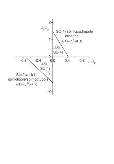
Figure 4: The phase diagram for the effective model in the strong coupling limit. ASL stands for algebraic spin liquid and $J_{-}=J_{2}-J_{1}$.

Now let us map out a ground state phase diagram of the model, which is shown in Fig. 4. When $c_{0}\gg|c_{2}|$ and $c_{0}\gg t$, we have $|J_{-}|\sim t^{2}|c_{2}|/c_{0}^{2}\ll|c_{2}|$ and $J_{3}\sim c_{2}$. Thus a stable $\pi$-flux state with spin algebraic correlations may be observed in the region that $|c_{2}|$ is comparable to $t^{2}/c_{0}$, implying that the competition of the exchange interaction between different sites and the on-site spin dependent interaction determines the low energy physics in the critical region. Furthermore, two second-order phase transitions occur along the two phase boundary curves, respectively. We would like to emphasize that there is no direct phase transition between the spin-quadrupole ordering and spin-dipole/spin-octupole ordering states.

VI Discussion

We have considered Mott insulating phases of spin-$\frac{3}{2}$ fermionic atoms in two-dimensional square optical lattices at half filling. In addition to the spin-quadrupole ordering phase, we found a degenerate antiferromagnetic spin-dipole/spin-octupole ordering phase. This is a symmetry breaking phase with the Goldstone manifold SO(5)/[SU(2)$\times$U(1)]=CP³ and six Goldstone bosonic modes. Compared to spin-quadrupole ordering phase, the time reversal symmetry is broken, and there are coupled transverse bosonic modes, which result in a suppression of the density wave velocity in the strong coupling limit. The topological properties in the two symmetry breaking phases are quite different: the spin-quadrupole ordering state contains a non-abelian SU(2) Berry phase and is characterized by the second Chern number, while the degenerate spin-dipole/spin-octupole ordering state contains only abelian U(1) Berry phase and is described by the first Chern number.

Due to these fundamental differences, a continuous phase transition from one to another is almost impossible (although a first order transition cannot be excluded in principle). Between these two phases, the quantum fluctuations are so strong that an SU(4) $\pi$-flux spin liquid state may be regarded as a quantum critical phase. In the low energy excitations of the algebraic liquid phase, there emerge U(1) massless gauge field and fractionalized spin-$\frac{3}{2}$ gapless spinons. Both the equal-time correlation functions of the spin-quadrupole operators and the SO(5) adjoint operators display the same power law behavior at long distance. We expect these features can be detected by spatial noise correlation experiments in future. We should mention that the above results were obtained in the mean field theory and more precise treatment of quantum fluctuations may modify the scenario.

- (1) M. Greiner, O. Mandel, T. Esslinger, T. W. Hänsch, and I. Bloch, Nature (London) 415, 39 (2002).
- (2) E. Demler and F. Zhou, Phys. Rev. Lett. 88, 163001 (2002).
- (3) F. Zhou and M. Snoek, Ann. Phys. (N.Y.) 308, 692 (2003); M. Snoek and F. Zhou, Phys. Rev. B 69, 094410 (2004).
- (4) A. Imambekov, M. Lukin, and E. Demler, Phys. Rev. A 68, 063602 (2003).
- (5) S. K. Yip, Phys. Rev. Lett. 90, 250402 (2003).
- (6) J. S. Bernier, K. Sengupta, and Y. B. Kim, Phy. Rev. B 74, 155124 (2006).
- (7) F. Zhou and G. W. Semenoff, Phys. Rev. Lett. 97, 180411 (2006).
- (8) K. Eckert, L. Zawitkowski, M. J. Leskinen, A. Sanpera, M. Lewenstein, cond-mat/0603273.
- (9) A. Widera, F. Gerbier, S. Fölling, T. Gericke, O. Mandel, and I. Bloch, Phys. Rev. Lett. 95, 190405 (2005).
- (10) H. J. Huang and G. M. Zhang, cond-mat/0601188.
- (11) J. S. Bernier, K. Sengupta, and Y. B. Kim, cond-mat/0612044.
- (12) A. Klein and D. Jaksch, Phys. Rev. A 73, 053613 (2006).
- (13) T. Fukuhara, Y. Takasu, M. Kumakura, and Y. Takahashi, Phys. Rev. Lett. 98, 030401 (2007).
- (14) C. Wu, J. P. Hu, and S. C. Zhang, Phys. Rev. Lett. 91, 186402 (2003).
- (15) C. Wu, Mod. Phys. Lett. B 20, 1707 (2006).
- (16) C. Wu, Phys. Rev. Lett. 95, 266404 (2005).
- (17) C. Wu, J. P. Hu, and S. C. Zhang, cond-mat/0512602.
- (18) H. H. Tu, G. M. Zhang, and L. Yu, Phys. Rev. B 74, 174404 (2006).
- (19) M. Hermele, T. Senthil, and M. P. A. Fisher, Phys. Rev. B 72, 104404 (2005).
- (20) W. Rantner and X. G. Wen, Phys. Rev. Lett. 86, 3871 (2001); W. Rantner and X. G. Wen, Phys. Rev. B 66, 144501 (2002).
- (21) R. Moessner and S. L. Sondhi, Phys. Rev. B 68, 184512 (2003).
- (22) X. G. Wen, Phys. Rev. B 68, 115413 (2003).
- (23) M. Hermele, M. P. A. Fisher, and L. Balents, Phys. Rev. B 69, 064404 (2003).
- (24) C. Xu, Phys. Rev. B 74, 224433 (2006); cond-mat/0602443.
- (25) C. Xu and M. P. A. Fisher, cond-mat/0611620.
- (26) F. Wilczek and A. Zee, Phys. Rev. Lett. 52, 2111 (1984); A. Zee, Phys. Rev. A 38, 1 (1988).
- (27) E. Demler and S. C. Zhang, Ann. Phys. (N.Y.) 271, 83 (1999).
- (28) C. H. Chern, H. D. Chen, C. Wu, J. P. Hu, and S. C. Zhang, Phys. Rev. B 69, 214512 (2004).
- (29) N. Nagaosa, Quantum Field Theory in Strongly Correlated Electronic Systems (Springer-Verlag, Berlin, 1999).
- (30) M. V. Berry, Proc. R. Soc. London, Ser. A 392, 45 (1984).
- (31) I. Affleck and J. B. Marston, Phys. Rev. B 37, 3774 (1988); J. B. Marston and I. Affleck, ibid. 39, 11538 (1989).
- (32) M. Hermele, T. Senthil, M. P. A. Fisher, P. A. Lee, N. Nagaosa, and X. G. Wen, Phys. Rev. B 70, 214437 (2004).
- (33) F. F. Assaad, Phys. Rev. B 71, 075103 (2005).
- (34) E. Altman, E. Demler, and M. D. Lukin, Phys. Rev. A 70, 013603 (2004).
- (35) S. Fölling, F. Gerbier, A. Widera, O. Mandel, T. Gericke, and I. Bloch, Nature (London) 434, 481 (2005).
- (36) T. Senthil, A. Vishwanath, L. Balents, S. Sachdev, and M. P. A. Fisher, Science 303, 1490 (2004); T. Senthil, L. Balents, S. Sachdev, A. Vishwanath, and M. P. A. Fisher, Phys. Rev. B 70, 144407 (2004).