Hybrid path integral Monte Carlo simulation of rigid diatomic molecules: effect of quantized rotations on the selectivity of hydrogen isotopes in carbon nanotubes

Abstract

We present a multiple time step algorithm for hybrid path integral Monte Carlo simulations involving rigid linear rotors. We show how to calculate the quantum torques needed in the simulation from the rotational density matrix, for which we develop an approximate expression suitable in the case of heteronuclear molecules.

We use this method to study the effect of rotational quantization on the quantum sieving properties of carbon nanotubes, with particular emphasis to the para-T₂/para-H₂ selectivity at 20 K. We show how to treat classically only some of the degrees of freedom of the hydrogen molecule and we find that in the limit of zero pressure the quantized nature of the rotational degrees of freedom greatly influence the selectivity, especially in the case of the (3,6) nanotube, which is the narrowest tube that we have studied.

We also use path integral Monte Carlo simulations to calculate adsorption isotherms of different hydrogen isotopes in the interior of carbon nanotubes and the corresponding selectivity at finite pressures. It is found that the selectivity increases with respect to the zero pressure value and tends to a constant value at saturation. We use a simplified effective harmonic oscillator model to discuss the origin of this behavior.

I Introduction

Carbon nanotubes have received a lot of attention in the past years in many fields of science and engineering, ranging from metallic properties, to adsorption of light gases.

The availability of these potentially narrow (subnanometer) channels has raised the interest about the possibility of using them as isotope sieves. The presence of quantum effects on adsorption has been known for quite a long time Katorski and White (1964); Moiseyev (1975) and Krylov et al. Beenakker et al. (1995) were the first to show, in the framework of a simple rigid wall model, the possibility of separating helium and hydrogen isotopes by using the different zero-point energy of the two confined species.

The idea was developed by Johnson and collaborators Wang et al. (1999); Challa et al. (2001, 2002), with particular emphasis about the calculation of the selectivity of T₂/H₂ mixtures in the interior channels of carbon nanotubes. These authors used an interaction potential model which neglects the molecular structure of hydrogen and developed a method - known as the simple theory - to calculate the selectivity in the limit of zero pressure (i.e. neglecting hydrogen-hydrogen interactions) by using the single particle energy levels in the confined system. Wang et al. (1999); Challa et al. (2001)

They conclude that the (3,6) nanotube would be able to show a selectivity of the order of 10⁵ at zero pressure and 20 K and calculated the expected selectivities for a wide set of nanotubes, thus displaying the dependence of this quantity on the radius of the tubes. They later extended their calculations, using path integral Monte Carlo methods, to finite pressures. Challa et al. (2002)

Hathorn et al. Hathorn et al. (2001) were the first to address the effect of the rotational degrees of freedom of hydrogen on the selectivity. Assuming a decoupling of the rotational and translational motions they showed that in narrow tubes one can expect an increase of the selectivity in narrow tubes of a factor 100 at 20 K, when compared with models that approximate hydrogen as a sphere.

These results have been confirmed by Trasca et al. Trasca et al. (2003), who calculated the D₂/H₂ selectivity in the interstitial channels and groove sites of various carbon nanotubes bundles.

Lu et al. Lu et al. (2003) have also calculated, in the framework of the simple theory, the energy levels and selectivity of molecular hydrogen in carbon nanotubes, by numerical diagonalization of the Schrödinger equation of a confined rotor, finding a value of the total selectivity for T₂/H₂ mixtures at zero pressure and 20 K of the order of 100 in the (3,6) tube, a result far lower than the ones already published in the literature. This result was later attributed to the use of an unphysical potential for the hydrogen-carbon interaction. Calculations with more realistic potentials Garberoglio et al. (2006); Lu et al. (2006) have confirmed the expectation of high selectivity.

Two problems seem still without a definite solution: the first is the effectiveness of model potentials in describing the carbon-hydrogen interactions. Different authors have used different potentials, and their predicted values of the selectivity scatter in an enormous range, from 10² to 10⁷. The second point, quite related to the first, is the actual effect of the rotational degrees of freedom on the selectivity.

We have addressed both these issues in a recent paper Garberoglio et al. (2006), where, in the framework of the simple theory, we have calculated the dependence of the zero pressure selectivity on the hydrogen-carbon interaction potential and we have developed an approximate method to evaluate the contribution of rotational-translational coupling to the selectivity itself.

We have demonstrated that the zero pressure selectivity is very much dependent on even small changes in the interaction potential, especially in the case of narrow tubes. Moreover the presence of a steep confining potential results in a strong translational-rotational coupling, and the overall selectivity cannot be calculated neither by assuming independence between those two degrees of freedom nor by assuming a spherically symmetric model for the hydrogen molecule. These results have been validated by the exact diagonalization of the hydrogen-carbon Hamiltonian reported in a recent paper by Lu et al. Lu et al. (2006)

In this paper we address the issue of the contribution of rotational degrees of freedom in more detail, using the path integral Monte Carlo method to treat the quantized rotational degrees of freedom in an exact way. After discussing how to perform an efficient path integral simulation of rotors using the hybrid Monte Carlo (HMC) technique, we develop a method for the classical treatment of the rotational degrees of freedom only and show that it gives a much lower zero pressure selectivity than the full quantum model. We also extend the calculations at finite pressures and discuss how the selectivity changes in this regime.

This paper is organized as follows. In Sec. II we describe the hybrid Monte Carlo method that we have used in this work. We further address the issue on how the zero pressure selectivity can be calculated from path integral simulations, with particular emphasis to the influence of the quantized rotational degrees of freedom. We develop a formalism that enables one to simulate classical rotations together with quantized center of mass degrees of freedom using a path integral approach and use this method to investigate the effect of the quantized rotational degrees of freedom on the selectivity..

In Sec. III we present and discuss our results. Some technical derivations are presented in the appendices.

II The hybrid path integral Monte Carlo method

II.1 The path integral formulation of statistical mechanics

The quantum mechanical expression for the partition function of a system of $N$ rigid linear rotors is

$$Q=\int d^{3N}X_{1}d^{2N}\Omega_{1}~{}\langle X_{1}\Omega_{1}|\exp[-\beta\hat{H}]|X_{1}\Omega_{1}\rangle$$ (1)

where we denote with $X$ a vector with the $3N$ center of mass coordinates of the rotors, and with $\Omega$ the set of the $2N$ angles describing their orientations. A subscript $1$ has been introduced for later convenience. The Hamiltonian $\hat{H}$ is given by

$$\hat{H}=\sum_{i=1}^{N}-\frac{\hbar^{2}}{2M}\nabla_{i}^{2}+\sum_{i=1}^{N}\frac{\hat{L}_{i}^{2}}{2I}+\sum_{i<j}v({\hat{x}}_{i}{\hat{\omega}}_{i};{\hat{x}}_{j}{\hat{\omega}}_{j})+\sum_{i=1}^{N}v_{\rm ext}({\hat{x}}_{i}{\hat{\omega}}_{i})$$ (2)

and is a function of the mass $M$, the angular momentum ${\hat{L}}$ and the inertia moment $I$ of the molecules. We have introduced a fluid-fluid pair interaction potential $v$ and a solid-fluid interaction potential $v_{\rm ext}$. The quantities ${\hat{x}}_{i}$ and ${\hat{\omega}}_{i}$ denote the operators for the center of mass position and the orientation of molecule $i$, respectively. The Hamiltonian is, as usual, the sum of the translational (center of mass) kinetic energy $\hat{T}$, the rotational kinetic energy $\hat{K}$, the fluid-fluid potential energy $\hat{V}$ and the solid-fluid potential energy $\hat{V}_{\rm ext}$.

The quantum partition function of Eq. (1) can be rewritten using repeatedly the Trotter identity

$$\exp[A+B]=\lim_{P\rightarrow\infty}\left(\exp[A/P]~{}\exp[B/P]\right)^{P}$$ (3)

valid for generally non-commuting operators $A$ and $B$ and further approximated by assuming a large but finite Trotter number $P$, obtaining

$$Q\simeq\int d^{3N}X_{1}d^{2N}\Omega_{1}~{}\langle X_{1}\Omega_{1}|\prod_{j=1}^{P}\exp(-\beta\hat{T}/P)\exp(-\beta\hat{K}/P)\exp[-\beta(\hat{V}+\hat{V}_{\rm ext})/P]|X_{1}\Omega_{1}\rangle$$ (4)

We can now introduce $P-1$ completeness relations of the form

$${\mathbf{1}}=\int d^{3N}X_{i}d^{2N}\Omega_{i}~{}|X_{i}\Omega_{i}\rangle\langle X_{i}\Omega_{i}|$$ (5)

between the factors in Eq. (4) and write the partition function as

$$Q \simeq \ \int d^{3N}X_{1}d^{2N}\Omega_{1}\ldots d^{3N}X_{P}d^{2N}\Omega_{P}$$ (6)

$$\langle X_{1}\Omega_{1}|\exp(-\beta\hat{T}/P)\exp(-\beta\hat{K}/P)\exp[-\beta(\hat{V}+\hat{V}_{\rm ext})/P]|X_{2}\Omega_{2}\rangle$$

$$\langle X_{2}\Omega_{2}|\exp(-\beta\hat{T}/P)\exp(-\beta\hat{K}/P)\exp[-\beta(\hat{V}+\hat{V}_{\rm ext})/P]|X_{3}\Omega_{3}\rangle$$

$$\ldots$$

$$\langle X_{P}\Omega_{P}|\exp(-\beta\hat{T}/P)\exp(-\beta\hat{K}/P)\exp[-\beta(\hat{V}+\hat{V}_{\rm ext})/P]|X_{1}\Omega_{1}\rangle$$

$$= \int d^{3N}X_{1}d^{2N}\Omega_{1}\ldots d^{3N}X_{P}d^{2N}\Omega_{P}$$

$$\prod_{t=1}^{P}\langle X_{t}\Omega_{t}|\exp(-\beta\hat{T}/P)\exp(-\beta\hat{K}/P)\exp[-\beta(\hat{V}+\hat{V}_{\rm ext})/P]|X_{t+1}\Omega_{t+1}\rangle$$

where we have denoted $X_{P+1}=X_{1}$ and $\Omega_{P+1}=\Omega_{1}$. Each of the matrix elements appearing in the previous equation can be written as

$$\langle X_{i}\Omega_{i}|\exp(-\beta\hat{T}/P)\exp(-\beta\hat{K}/P)\exp[-\beta(\hat{V}+\hat{V}_{\rm ext})/P]|X_{i+1}\Omega_{i+1}\rangle =$$

$$\langle X_{i}|\exp(-\beta\hat{T}/P)|X_{i+1}\rangle~{}\langle\Omega_{i}|\exp(-\beta\hat{K}/P)|\Omega_{i+1}\rangle~{}\exp[-\beta(V(X_{i+1}\Omega_{i+1})+V_{\rm ext}(X_{i+1}\Omega_{i+1}))/P]$$ (7)

A straightforward calculation shows that the expectation value of the translational kinetic energy Boltzmann factor assumes the form Landau and Binder (2000)

$$\langle X_{i}|\exp(-\beta\hat{T}/P)|X_{i+1}\rangle=a\exp(-\beta\kappa|X_{i}-X_{i+1}|^{2}/2)$$ (8)

where the amplitude $a$ and the “spring constant” $\kappa$ are given by

$$a = \left(\frac{Mk_{B}TP}{2\pi\hbar^{2}}\right)^{3/2}$$ (9)

$$\kappa = \frac{MP(k_{B}T)^{2}}{\hbar^{2}}$$ (10)

and the expectation value of the rotational kinetic energy Boltzmann factor becomes Marx and Müser (1999)

$$\langle\Omega_{i}|\exp(-\beta\hat{K}/P)|\Omega_{i+1}\rangle = \sum_{n=1}^{N}\sum_{J=0}^{\infty}\frac{2J+1}{4\pi}P_{J}(\cos\theta^{n}_{i,i+1})\exp[-\beta J(J+1)B/P]$$ (11)

$$\equiv \sum_{n=1}^{N}\Xi(\theta^{n}_{i,i+1})$$

where $P_{J}(\cdot)$ is a Legendre polynomial, $\theta^{n}_{i,i+1}$ is the angle between the directions $\omega_{i}$ and $\omega_{i+1}$ relative to molecule $n$ and $B=\hbar^{2}/(2I)$ is the rotational constant of the rotor. In the case of homonuclear molecules the indistinguishability of the nuclei imposes some restrictions on the sum in Eq. (11) according to the spin states of the nuclei: for para-H₂, ortho-D₂ and para-T₂, as in this work, the summation on the angular momenta $J$ in Eq. (11) is limited to the even numbers only Marx and Müser (1999) and results in a positive definite density matrix, which can be directly used in the Monte Carlo simulations.

In the other rotational states (i.e. ortho-H₂ and T₂ and para-D₂) the sum is restricted to the odd angular momentum states, resulting in a density matrix which is not positive definite. As a consequence, more care has to be taken in performing a Monte Carlo simulation in this case Marx and Müser (1999).

The net effect of these algebraic manipulations is that we have been able to rewrite the original quantum partition function of an $N$ particle system, Eq. (1), as a classical partition function of a $NP$ particle systems. The $NP$ particle of the classical equivalent are naturally divided in $P$ subsets (also known as time slices) of $N$ particles each. Each particle in a time slice interacts with all the other particles in the same time slice via the original intermolecular and intramolecular potential divided by a factor of $P$ (see Eq. (7)). Quantum mechanical effects taken into account by the interaction of each particle with the corresponding copy on the previous and following time slice: the center of mass coordinates are bound by the harmonic potential of Eq. (8) and the orientations give rise to the inter-slice rotational partition function of Eq. (11). The resulting system is then equivalent to a classical collection of $N$ ring polymers, each having $P$ beads. The $i$-th particle on a given polymer interacts only with the corresponding particle on the other polymers via the original intermolecular potential (rescaled by a factor of $P$). The interaction between the beads of a given ring polymer are described by an harmonic interaction on the translational coordinates with the two adjacent beads (see Eq. (8)) and an interaction between the orientational degrees of freedom of adjacent beads whose density matrix is given by Eq. (11).

II.2 Observables and estimators

In the framework of the path integral approximation to the quantum partition function the estimators for the average values of interest can usually be obtained by their thermodynamic definitions.

The estimator for the translational kinetic energy is then Landau and Binder (2000)

$$T^{\rm est}=\frac{3}{2}k_{B}TP-U_{\rm quant}$$ (12)

where $U_{\rm quant}=(\kappa/2)\sum_{t=1}^{P}|X_{t}-X_{t+1}|^{2}$ is the value of the quantum spring potential energy, and the one for the rotational kinetic energy is Marx and Müser (1999)

$$K^{\rm est} = \frac{1}{P}\sum_{i=1}^{P}K^{\rm est}_{i}$$ (13)

$$K^{\rm est}_{i} = \frac{B}{4\pi\Xi}\sum_{J}J(J+1)(2J+1)~{}P_{J}(\cos\theta_{i~{}i+1})\exp\left(-\frac{\beta}{P}BJ(J+1)\right)$$ (14)

We can derive an expression for the calculation of the particle density in a path integral simulation. Denoting $\hat{x}^{(t)}_{i}$ as the position operator of particle $i$ in time slice $t$, one has

$$\rho(r) = \langle\sum_{n=1}^{N}\frac{1}{N}\delta(r-\hat{x}_{n})\rangle$$ (15)

$$= \frac{1}{Q}\int d^{3N}X_{1}d^{2N}\Omega_{1}~{}\langle X_{1}\Omega_{1}|\sum_{n=1}^{N}\frac{1}{N}\delta(r-\hat{x}^{(1)}_{n})\exp[-\beta\hat{H}]|X_{1}\Omega_{1}\rangle$$ (17)

$$= \frac{1}{Q}\int d^{3N}X_{1}d^{2N}\Omega_{1}~{}\sum_{n=1}^{N}\frac{1}{N}\delta(r-x^{(1)}_{n})\times$$

$$\langle X_{1}\Omega_{1}|\prod_{j=1}^{P}\exp(-\frac{\beta}{P}\hat{T})\exp(-\frac{\beta}{P}\hat{K})\exp[-\frac{\beta}{P}(\hat{V}+\hat{V}_{\rm ext})]|X_{1}\Omega_{1}\rangle$$

introducing now $P-1$ completeness relations, analogously to the passage leading to Eq. (6) and noting that the integrand can be rewritten by relabeling $X_{1}\leftrightarrow X_{j}$, one obtains from Eq.(17)

$$\rho(r) = \frac{1}{Q}\int\prod_{p=1}^{P}d^{3N}X_{p}d^{2N}\Omega_{p}\left(\frac{1}{NP}\sum_{t=1}^{P}\sum_{n=1}^{N}\delta(r-x^{(t)}_{n})\right)\times$$ (18)

$$\prod_{p=1}^{P}\langle X_{p}\Omega_{p}|\exp(-\frac{\beta}{P}\hat{T})\exp(-\frac{\beta}{P}\hat{K})\exp[-\frac{\beta}{P}(\hat{V}+\hat{V}_{\rm ext})]|X_{p+1}\Omega_{p+1}\rangle$$

so that the density at a point $r$ is equivalent to the probability of finding the center of mass of a bead at the same point.

II.3 The hybrid Monte Carlo method

Using the path integral formulation, a quantum partition function can be rewritten as a classical partition function of a system with a larger number of particles, so that classical Monte Carlo methods can then be used to calculate thermodynamic properties. Since we expect to work at conditions where quantum mechanics is not a small correction, it will be necessary to use large values of the Trotter number $P$. A simple Metropolis method for the sampling of the translational and rotational phase space, such as the one discussed in Ref. Cui et al., 1997, will be affected by slow convergence. We have then decided to use the hybrid Monte Carlo method, Duane et al. (1987); Tuckerman et al. (1993) that consists in choosing a new candidate configuration by performing a molecular dynamics (MD) move with a large timestep; the resulting configuration is then accepted or rejected using a standard Metropolis condition on the difference in the total energy (which is not conserved if a large enough timestep is taken).

In order to perform an MD move one has to know the forces and the torques acting on each of the rotors. The potential energy between the molecules on the same slice is given by the rescaled original potential, and the quantum mechanical effects on the translational degrees of freedom are described by a simple harmonic potential between adjacent slices (see Eq. (8)). The only unknown is the quantum torque between the molecules in adjacent slices: we have decided to calculate it numerically, starting from the expression of the density matrix in Eq. (11) (see Appendix B for an analytic limit in the case of heteronuclear molecules). Since Eq. (11) represents a Boltzmann factor it can generally be written as $B_{\rm rot}=C\exp[-\beta U_{\rm rot}(\theta)]$ where $C$ is an unknown constant and $U_{\rm rot}(\theta)$ is the quantum rotational potential energy between two adjacent rotors, whose orientations form an angle $\theta$ with one another; we show in the appendix that for heteronuclear molecules in the high $P$ limit $U_{\rm rot}$ is given to a good approximation by the harmonic expression $U_{\rm rot}(\theta)=K\theta^{2}/2$ with $K$ given in Eq. (40). In the general case the modulus of the quantum torque can be written as

$$N_{\rm quant}(\theta)=-\frac{dU_{\rm rot}(\theta)}{d\theta}=\frac{k_{B}T}{\Xi}\sin\theta\frac{d\Xi(\theta)}{d\cos\theta}$$ (19)

The direction of the torque is obviously orthogonal to the plane generated by the two orientations of the interacting molecules, and such that it tends to close the angle between the two molecules. The derivative in Eq. (19) could be evaluated either numerically or using the identity

$$\frac{dP_{l}(x)}{dx}=\frac{lxP_{l}(x)-lP_{l-1}(x)}{x^{2}-1}$$

II.4 The multiple time step method

Inspection of Eqs. (7) and (10) shows that the intermolecular forces scale like the inverse of the Trotter number $P$, whereas the quantum forces (and, possibly, the torques) are proportional to it. In order to efficiently sample phase space using an hybrid Monte Carlo method it is necessary that all the degrees of freedom contribute uniformly to the non-conservation of energy when a MD time step is performed. Since the intermolecular forces become weaker for large Trotter number while the quantum forces become stronger, we have decided to use a multiple time step method to perform the MD evolution. Tuckerman et al. (1992) We divide the forces into “long range” (the intermolecular forces, in our case) and “short range” (the quantum forces and torques). Each of the long range dynamical steps $\Delta t$ is divided into $n$ smaller time steps $\delta t$ where only the short range forces are evaluated as the system is propagated.

In our case we do not know the typical time scale of the quantum rotation, so we have decided to use three nested loops: we use a long time step $\Delta t$ to propagate the system according to the intermolecular forces, an intermediate time step $\delta t$ to propagate the quantum spring forces on the translational degrees of freedom and a rotational time step $\delta\tau$ to propagate the quantum torques.

We also need, for the hybrid method to work, a reversible algorithm to integrate all the degrees of freedom. It is well known that the velocity form of the Verlet algorithm possess such a feature and can be used in multiple time step methods. Tuckerman et al. (1992) Instead of using algorithms already developed to treat the general motion of rigid rotors in a multiple time step framework Matubayasi and Nakahara (1999) we have developed a velocity Verlet like integrator for the rotational motion of a rigid linear rotor that can be easily integrated in the velocity Verlet evolution of the center of mass coordinates. Details of its derivation are given in Appendix A.

Denoting by $x$ and $v$ the translational positions and velocities, and by $e$ and $\varpi$ the direction of the molecular axes and the molecular angular velocities, the multiple time step method is then implemented as follows:

Calculate $F_{long}$ and $N_{long}$ (intermolecular forces)
$v\rightarrow v+\Delta tF_{long}/(2M)$
$\varpi\rightarrow\varpi+\Delta tN_{long}/(2I)$
	Calculate $F_{short}$ (quantum spring)
	$v\rightarrow v+\delta tF_{short}/(2M)$
		Calculate $N_{short}$ (quantum torque)
		$\varpi\rightarrow\varpi+\delta\tau N_{long}/(2I)$
		$e\rightarrow e+\delta\tau~{}\varpi\times e-(\delta\tau)^{2}\varpi^{2}/2$
		normalize $e$
		Calculate $N_{short}$ (quantum torque)
		$\varpi\rightarrow\varpi+\delta\tau N_{long}/(2I)$
		$x\rightarrow x+v\delta\tau$
	Calculate $F_{short}$
	$v\rightarrow v+\delta tF_{short}/(2M)$
Calculate $F_{long}$ and $N_{long}$
$v\rightarrow v+\Delta tF_{long}/(2M)$
$\varpi\rightarrow\varpi+\Delta tN_{long}/(2I)$
Calculate the final translational and rotational kinetic energy

In order to fix the integer values of the ratios $\delta t/\delta\tau$ and $\Delta t/\delta t$ we have proceeded as follows. For the first ratio we have performed some ideal gas simulations, where the translational and rotational motions are decoupled and can be simulated by taking into account translations and rotations separately. We have adjusted the rotational and translational ideal gas time steps in order to have a 50% acceptance ratio and we have then fixed $\delta t/\delta\tau=(\delta t/\delta\tau)_{\rm ideal\ gas}\simeq 3$.

The ratio $\Delta t/\delta t$ is more difficult to set, but as a first guess one can set it equal to the inverse ratio of the Einstein frequencies corresponding to the intramolecular and quantum forces, that we calculate during the course of the simulations. For particles confined in narrow tubes we found that the optimal ratio $\Delta t/\delta t$ is of the order of 8-10. There are at least two possible strategies for the parallelization of the multiple time step algorithm for rigid rotors. In the first case, one can distribute the number of beads among the available nodes, and in the second case one can distribute the number of molecules. Using the first method requires very frequent and very short messages to be passed between the nodes, i.e. every short time step $\delta\tau$. In the second case the quantum dynamics is performed locally, but the positions of all the molecules have to be redistributed among the nodes at every long time step in order to calculate the intermolecular forces: this results in less frequent communications (i.e. every long time step $\Delta t$), but the amount of data for a single communication is larger than in the first case. In the case of non-interacting molecules (i.e. the zero pressure limit) the last strategy results, of course, in a negligible amount of inter-node communication and is therefore optimal.

II.5 Calculation of the selectivity

The selectivity of two components, say T₂ and H₂ is defined as:

$$S(T_{2}/H_{2})=\frac{x_{T_{2}}/x_{H_{2}}}{y_{T_{2}}/y_{H_{2}}},$$ (20)

where $x$ and $y$ are the mole fractions in the adsorbed and bulk phases, respectively.

In the limit of zero pressure, when one can neglect the adsorbate–adsorbate interaction, the selectivity depends only on the energy levels $E^{l}$ of the adsorbed molecules, and can be written as Challa et al. (2002); Hathorn et al. (2001)

$$S_{0}(T_{2}/H_{2})=\frac{Q_{H_{2}}^{\rm free}}{Q_{T_{2}}^{\rm free}}\frac{Q_{T_{2}}}{Q_{H_{2}}}=\left(\frac{m_{H_{2}}}{m_{T2}}\right)^{d/2}\frac{Q_{T_{2}}^{\rm free-rot}}{Q_{H_{2}}^{\rm free-rot}}\left[\frac{\displaystyle\sum_{l}\mathrm{exp}{\left(-E_{T_{2}}^{l}/kT\right)}}{\displaystyle\sum_{l}\mathrm{exp}{\left(-E_{H_{2}}^{l}/kT\right)}}\right]$$ (21)

where $Q^{\rm free}$ is the molecular partition function for the ideal gas, $Q^{\rm free-rot}$ is the free rotor molecular partition function and $Q$ is the molecular partition function for the given specie. We have denoted by $d$ the number of spatial dimensions in which confinement takes place. In the case of hydrogen molecules in carbon nanotubes, $d=2$. In the zero pressure limit the selectivity is a function of the energy levels of the two species, which can be obtained by a direct diagonalization of the single-particle Hamiltonian. We shall refer to this procedure as “the simple model”.

We notice that, under the assumption that the rotational and translational dynamics are independent, one can rewrite Eq. (21) as

$$S_{0}(T_{2}/H_{2})\simeq\left(\frac{m_{H_{2}}}{m_{T_{2}}}\frac{Q_{T_{2}}^{\rm tras}}{Q_{H_{2}}^{\rm tras}}\right)\left(\frac{Q_{T_{2}}^{\rm free-rot}}{Q_{H_{2}}^{\rm free-rot}}\frac{Q_{T_{2}}^{\rm rot}}{Q_{H_{2}}^{\rm rot}}\right)=S_{0}^{\rm tras}S_{0}^{\rm rot}$$ (22)

The calculation of the selectivity of a confined T₂/H₂ can in principle be performed using the definition given in Eq. (20), evaluating the mole fractions in the bulk and in the confined system using Grand Canonical Monte Carlo simulations.

Since we expect quite high selectivities (possibly of the order of $10^{5}$ or more), the evaluation of the mole fraction would require the simulation of very large systems, of the order of at least $10^{5}$ molecules. In order to avoid the use of such demanding calculations, we have employed the method developed by Challa et al. Challa et al. (2001); Wang et al. (1997) to evaluate the zero pressure selectivity. With a straightforward extension to rigid rotors the selectivity in the limit of zero pressure can be written as

$$S_{0}({\mathrm{T}}_{2}/{\mathrm{H}}_{2})=C~{}\langle\exp[-\beta\Delta U_{{\mathrm{H}}_{2}\rightarrow{\mathrm{T}}_{2}}]\rangle_{{\mathrm{H}}_{2}}$$ (23)

where

$$\Delta U_{{\mathrm{H}}_{2}\rightarrow{\mathrm{T}}_{2}}=\int_{m_{H2}}^{m_{T2}}dm~{}\left(\frac{dU_{int}}{dm}\right)$$ (24)

is the variation of the quantum potential energy when a H₂ molecule is gradually transformed into a T₂ molecule by performing a number $N_{MC}$ of Monte Carlo steps and the constant $C$ is given by

$$C=\frac{Q^{\rm free-rot}(H_{2})}{Q^{\rm free-rot}(T_{2})}\left(\frac{m_{T_{2}}}{m_{H_{2}}}\right)^{\frac{3}{2}(P-1)}\left(\frac{I_{T_{2}}}{I_{H_{2}}}\right)^{P}$$ (25)

where we have denoted by $I$ the inertia moment of a given specie, and the average in Eq. (23) is performed on a simulation of the lightest specie only. A number of the order of $N_{MC}=4000$ points are necessary to reach convergence in the evaluation of the integral in Eq. (24) for the H₂ to T₂ transformation.

In order to calculate the selectivity at finite pressures Challa et al. Challa et al. (2002) have developed an efficient method to perform Grand Canonical simulations of mixtures. The usual insertion and deletion moves are performed for the heavier specie only (T₂ in our case), whereas the lighter specie is inserted or deleted by performing T${}_{2}\leftrightarrow$ H₂ transformations. A transformation move of a molecule of the specie 1 into a molecule of the specie 2 is accepted with the probability

$${\cal P}_{1\rightarrow 2}={\rm min}\left[1,\frac{N_{1}}{N_{2}+1}\left(\frac{\Lambda_{1}}{\Lambda_{2}}\right)^{3}\exp[\beta(\mu_{2}-\mu_{1})]\exp[-\beta\Delta U^{\rm ext}]\right]$$ (26)

where $N$ is the number of molecules already present in the system, $\Lambda$ is the de Broglie wavelength, $\mu$ the chemical potential (which is different for the two species to account for a given bulk molar composition) and $\Delta U^{\rm ext}$ is the difference of the sum of the fluid-fluid and solid-fluid potential energies between the configurations $(N_{1},N_{2})$ and $(N_{1}-1,N_{2}+1)$. Note that, in order to fulfill the detailed balance condition, the probability of a T${}_{2}\rightarrow$ H₂ transformation attempt must be equal to the probability of attempting the reverse move.

II.6 Classical treatment of the rotational degrees of freedom

In order to assess the importance of the quantized rotational degrees of freedom in quantum sieving we now develop a formalism to describe a system in which only the translational degrees of freedom are quantized and the rotations are described classicaly.

In what follows we perform the derivation referring to a single rotor in an external potential, in order to avoid a cumbersome notation. The extension to interacting rotors is straightforward.

Consider a system whose Hamiltonian is given by $H=T(\hat{p})+K(\hat{L})+V({\hat{x}},{\hat{\Omega}})$, where $T({\hat{p}})={\hat{p}}^{2}/2m$ is the kinetic energy of translation, $K({\hat{L}})=B{\hat{L}}^{2}$ is the kinetic energy of rotation and $V({\hat{x}},{\hat{\Omega}})$ is the potential energy with a dependence on the position operator $\hat{x}$ of the center of mass and the direction $\hat{\Omega}$. The quantum mechanical partition function is given by

$$Q=\int dx\sum_{l,m}\langle x;l,m|\exp[-\beta(T+K+V)]|x;l,m\rangle$$ (27)

The classical treatment of some of the degrees of freedom correspond to the assumption that the operators of the corresponding generalized coordinates and momenta commute. Since we are interested in approximating the rotation as classical, we proceed as if the rotational kinetic energy and the potential, which depends on the molecular orientation, obey the commutation relation $[{\hat{V}},{\hat{K}}]=0$, which implies $\exp[-\beta(T+V+K)]=\exp[-\beta(T+V)]\exp[-\beta K]$. One can then perform the partial trace over the rotational degrees of freedom, obtaining

$$q = {\rm Tr}_{rot}\exp[-\beta(T+K+V)]$$ (28)

$$= \sum_{lm}\langle l,m|\exp[-\beta(T+K+V)]|l,m\rangle$$

$$= \sum_{lm}\langle l,m|\exp[-\beta(T+V)]|l,m\rangle~{}e^{-\beta Bl(l+1)}$$

$$= \int d\omega_{1}d\omega_{2}\sum_{lm}~{}\langle lm|\omega_{1}\rangle\langle\omega_{1}|\exp[-\beta(T+V)]|\omega_{2}\rangle\langle\omega_{2}|l,m\rangle~{}e^{-\beta Bl(l+1)}$$

$$= \int d\omega_{1}d\omega_{2}\sum_{lm}~{}Y^{*}_{lm}(\omega_{1})Y_{lm}(\omega_{2})\langle\omega_{1}|\omega_{2}\rangle\exp[-\beta(T+V(x,\omega_{2})]~{}e^{-\beta Bl(l+1)}$$

$$= \int d\omega_{1}\left(\sum_{l}\frac{2l+1}{4\pi}e^{-\beta Bl(l+1)}\right)\exp[-\beta(T+V(x,\omega_{1})]$$

$$= Q_{rot}\int\frac{d\omega}{4\pi}\exp[-\beta(T(\hat{p})+V(\hat{x},\omega))]$$

where $Q_{rot}$ is the molecular partition function of the free rotor. In the last expression the direction $\omega$ is the classical direction of the rotor and $\hat{p}$ and $\hat{x}$ are the momentum and position operators (still quantum mechanical).

When one applies the Trotter formula to the reduced density matrix $q$ each of the beads corresponding to a given molecule has the molecular axis pointing in the same direction as the others, since $\omega$ is now considered as a classical variable.

III Results and discussion

III.1 The potential model

In order to assess the importance of quantized rotation on the selectivity, we need a potential model that explicitely treats the hydrogen molecule as a rigid rotor. To the best of our knowledge no such model has been extensively tested in the literature. We have recently evaluated the zero pressure selectivity of various potential models in the (3,6) nanotube in the framework of the “simple theory”, that is, using Eq. (21) with the energy levels obtained by a direct diagonalization of the Hamiltonian. Garberoglio et al. (2006); Lu et al. (2006) Many models predict very high selectivities (in the range $10^{7}-10^{10}$), and we noticed a strong dependence of the selectivity on the potential parameters.

We have chosen to use a reasonable potential model, well aware of the fact that it might not be the best one to describe the actual interaction of hydrogen molecules with themselves and with a carbon nanotube. We would like to point out that our main interest in this work is to evaluate the effect of quantized degrees of freedom on the selectivity, and not to develop an accurate model to describe the hydrogen-carbon or hydrogen-hydrogen interaction.

We describe the hydrogen molecule as a rigid rotor of length $l=0.74$ Å with two Lennard-Jones sites on the position of the hydrogen atoms, having as parameters $\epsilon=8.4$ K and $\sigma=2.81$ Å. Murad and Gubbins (1978) The Lennard-Jones radius of this model is less than the Lennard-Jones radius of the Buch potential (where $\sigma_{\rm Buch}=2.96$ Å), which has been shown to be a good spherical potential to describe the bulk properties of hydrogen. The smaller $\sigma$ takes into account the fact that the potential has two centers, separated by a distance corresponding to the actual gas phase H₂ bond length. The value of $\epsilon$ is almost one fourth of the corresponding value for the Buch potential (where $\epsilon_{\rm Buch}=34.2$ K) and this takes into account the fact that in a site-site model we have actually four interactions between the two molecules.

We have also described the carbon atoms in the nanotubes with a Lennard-Jones potential, using the Steele parameters $\sigma_{C}=3.4$ Å and $\epsilon_{C}=28.0$ K. Steele (1978) Solid-fluid interactions have been calculated using the Lorentz–Berthelot mixing rules. We have generated carbon nanotubes of various sizes and tabulated the solid-fluid potential by averaging, in cylindrical coordinates, over the length of a unit cell in the direction $z$ of the tube axis and over the angle $\Phi$ in a plane orthogonal to the tube axis, thus obtaining the solid-fluid potential as a function of the distance of the molecule’s site from the nanotube axis only.

In this study we have focused our attention on the carbon nanotubes called (3,6), (2,8), (6,6) and (10,10) with the standard nomencalture. These tubes have geometrical radii of 3.1, 2.6, 4.1 and 5.1 Å, respectively. We report the profile of the potential energy with one of the hydrogen sites if Fig. 1.

Figure 1: The average potential energy curves for one of the hydrogen sites with the carbon nanotubes used in this study, as a function of the distance from the tube axis.

III.2 The zero pressure selectivity

Simulation	Selectivity	Solid-fluid PE (K)	Translational KE (K)	Rotational KE (K)
(3,6)	$6.34\times 10^{7}$	-648	320	109
(3,6) classical	27000	-900	280	–
(3,6) simple model	24400	-932	271.5	–
(2,8)	52	-1257	134	0
(2,8) classical	21	-1297	115	–
(2,8) simple model	17	-1313	98	–
(6,6)	2.3	-1016	66	0
(6,6) classical	2.3	-1018	55.7	–
(6,6) simple model	2.12	-1022	41.9	–
(10,10)	5.6	-524	71	0
(10,10) classical	4.2	-532	66	–
(10,10) simple model	4.7	-556	58.1	–

Table 1: The values of the para-T₂/para-H₂ selectivities calculated for different nanotubes at 20 K. The potential and kinetic energies reported are those of the H₂ molecule. The simple model results have been obtained by assuming that a molecule is aligned with the nanotube axis and that rotations do not contribute to the selectivity.

Our results for the influence of the quantization of the rotational degrees of freedom on the selectivity are shown in Table 1, where we report zero pressure selectivities and average energies for hydrogen confined in the (3,6), (2,8), (6,6) and (10,10) carbon nanotube.

The simulations have been performed using the method described in Eq. (23). A system of at least 50 non interacting molecules was equilibrated inside a carbon nanotube for at least 20000 HMC steps, and the selectivity was then calculated by performing a production run of at least 20000 HMC moves. The selectivity was calculated from Eq. (23), with configurations sampled every 50 HMC steps and using $N_{MC}=4000$ points for the integration of Eq. (24).

It is apparent that the explicit inclusion of the rotational degrees of freedom has a dramatic effect on the selectivity, especially in the narrowest tube, where it jumps from 27000 up to $6.34\times 10^{7}$, a more than 2000 fold increase. In the other tubes, the effect of the rotational degrees of freedom is less dramatic, being of the order of 2.5 in the (2,8) tube and almost negligible in the (6,6).

This enhancement is more than can be expected from a simple analysis that assumes independence of the translational and rotational degrees of freedom, Hathorn et al. (2001) which would give, in the case of the (3,6) tube with our potential, a selectivity 750 times higher than the one obtained assuming an isotropic potential. Garberoglio et al. (2006) Rotational-translational coupling effects must be taken into account in narrow carbon nanotubes. We would also like to point out that the actual magnitude of the rotational-translational coupling on the selectivity calculated with the path integral simulations is still higher than the one obtained using the approximate method that we have developed in Ref. Garberoglio et al., 2006, which would give, for the same system analyzed here, an enhancement of the selectivity by a factor of 1650.

The physical origin of the higher selectivity due to the quantization of the rotational degrees of freedom can be seen by analizying the difference between the simulations in which the rotational are treated classically and the ones in which the rotations are treated quantized.

In the presence of narrow confining potentials one expects to find the molecules aligned with the nanotube axis, when rotations are treated classically. In fact, we have calculated in Ref. Garberoglio et al., 2006 the selectivity in the framework of the simple model assuming a perfect alignment - so that the potential energy is a function of the center of mass position only - and we can see, from the results reported in Table 1, that the results are in very good agreement with the path integral simulations where rotational degrees of freedom are assumed to behave classically.

We have also calculated the average angle $\Theta$ between the molecular axis and the nanotube axis in the classical simulations as a function of the distance of the molecule from the nanotube axis. One can see from Fig. 2 that in the classical case one obtains $\Theta\simeq 8$ degrees, thus confirming an almost perfect alignement.

Figure 2: The average angle between the nanotube and the molecular axes as a function of the distance from the (3,6) nanotube center for H₂. Solid line, full quantum simulations. Dashed line, classical treatment of the rotational degrees of freedom.

The situation changes dramatically upon quantization of the rotational degrees of freedom, since the confining effect of the potential energy is now counterbalanced by the quantum delocalization. The average angle $\Theta$ between the “orientation” of a given bead and the nanotube axis averages around 35 degrees at the center of the tube and has a slight decrease towards 25 degrees for the molecules which happen to be off center, where the potential energy is steeper.

The effect of quantum fluctuations in the orientation can also be seen by the high value of the rotational kinetic energy reported in Table 1. Hydrogen molecules confined in the narrowest tube have an average rotational kinetic energy up to 109 K, a very high value when compared to the free-rotor rotational energy at the same temperature, which is about 0.1 K due to the freezing of the rotational degrees of freedom on the $l=0$ spherically symmetric ground state. Due to the confining potential that tends to localize the molecular direction along the nanotube axis, the rotational state of the adsorbed rotor is a superposition of higher angular momentum states, resulting in a non-zero value of the average kinetic energy.

If we now consider, in a semiclassical picture, a molecule at a given distance from the nanotube axis, we see that the quantization of the rotational degrees of freedom (and the consequent rotational delocalization) has the effect that the molecule samples region where the potential energy is higher with respect to an almost perfectly aligned (classical) configuration. One can then see that the average potential acting on the center of mass is steeper when rotations are quantized than in the case when rotations are treated classically, and that the steepness is higher for the lighter molecule than for the heavier one. As a consequence, the energy levels of the lighter rotors are more separated with respect to the energy levels of the heavier specie, not only because of a different mass, but also because the quantization of rotations has a different effect on the two kind of molecules. In the light of the simple theory formula, Eq. (21), we can then see that quantized rotations enhance the spacing between the energy levels with a greater effect on the light isotope, thus having a big effect on the selectivity, as is indeed observed in the simulations. This phaenomenon has been termed “extreme two dimensional confinement” by Lu et al. Lu et al. (2006) By a careful analysis of numerically exact eigenstates of hydrogen isotopes confined in carbon nanotubes, they found that a large value of the selectivity is to be expected in geometries so narrow that the rotational ground state takes contribution from states with finite angular momentum. We have been able to show, Garberoglio et al. (2006) using an approximate model for the description of the coupled rotational and translational degrees of freedom, that under these circumstances a very large contribution to the selectivity does indeed come from the rotational degrees of freedom, as is apparent in the exact result that we show in Table 1 for the (3,6) tube. In the other tubes the average rotational kinetic energy has been found to be zero within the error bars, and the contribution of the rotational degrees of freedom to the selectivity is correspondingly smaller.

One can also see the effect of the more confining effective potential by plotting the expected density of a molecule as a function of the distance from the tube center, when rotations are treated classically or quantized. We show the results for hydrogen in the (3,6) tube in Fig. 3, where it can be seen that the classical treatment of the rotational degrees of freedom results in a lower density along the tube axis, a signature of an effectively less confining external potential, as is also apparent from the average kinetic and potential energies reported in Table 1: the quantized treatment of the rotational degrees of freedom results in higher average kinetic and potential energies, when compared to the case in which rotations are treated classically.

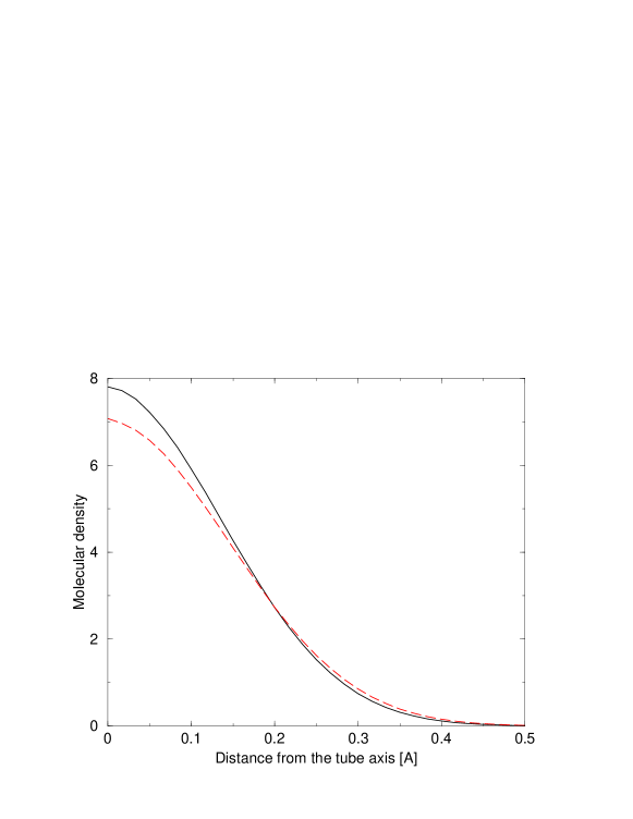
Figure 3: Normalized densities for hydrogen confined in the (3,6) tube at 20 K from Eq. (18). Solid line, quantum treatment of the rotational degrees of freedom. Dashed line, classical treatment of the rotational degrees of freedom

III.3 Adsorption isotherms

Using the path integral simulations we have calculated the adsorption isotherms for different hydrogen isotopes in the (3,6), (2,8) and (6,6) carbon nanotubes. The results are shown in Figs. 4 and 5.

As a general trend, we notice that the heavier specie is the one most readily adsorbed, as is expected. Qualitatively, one can think that the larger thermal de Broglie wavelength of the lighter specie results in a larger effective Lennard-Jones radius, thus hindering the adsorption.

Quantum effects result in a separation in pressure between the isotherms of different isotopes. This is a negligible effect in large tubes, such as the (6,6) where quantum mechanical effects do not influence the adsorption very much (as apparent from the low selectivity). In this case the isotherms of the different isotopes are very close, as can be seen in Fig. 4.

The opposite is observed in the very confining (3,6) tube. It can be seen in Fig. 4 that T₂ can be adsorbed already at $10^{-15}$ bar, whereas the adsorption of H₂ is not detectable below $10^{-5}$ bar, a difference of 10 orders of magnitude.

In the (2,8) tube we observe a sizeable presence of quantum effects, though not as dramatic as in the (3,6), the isotherms of the lightest and heaviest species are separated by two order of magnitude in pressure.

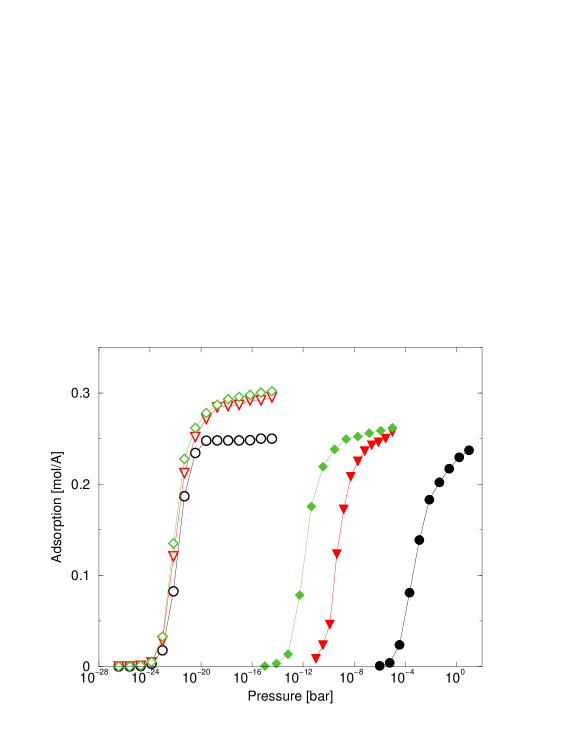
Figure 4: Pure fluid adsorption isotherms for hydrogen isotopes in the (3,6) (filled symbols) and (6,6) (open symbols) carbon nanotubes at 20 K. The circles and diamonds refer to para-H₂ and para-T₂ respectively, whereas the triangles refer to ortho-D₂. The lines are drawn as a guide for the eye.

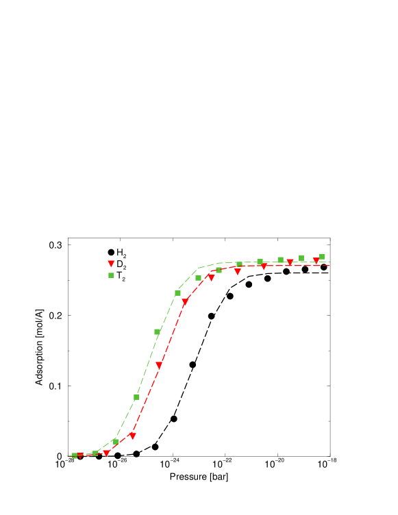
Figure 5: Pure fluid adsorption isotherms for hydrogen isotopes in the (2.8) carbon nanotube at 20 K. The circles, triangles and diamonds refer to para-H₂, ortho-D₂ and para-T₂ respectively. The lines are fit with the LUD isotherm.

These isotherms allow us to clarify in detail how low the pressure must be in order to fulfill the zero pressure limit discussed in the previous section. For a given nanotube we can take as an estimate the pressure for which the isotherm of the heavier specie starts to be significantly different from zero.

We notice that a high zero pressure selectivity is correlated with the separation in pressure of the isotherms corresponding to the two species. When the heavier molecules begins to be adsorbed, the lighter one cannot easily do so, hence the high values of the selectivity.

III.4 Selectivity at finite pressures

Using path integral simulations it is possible to investigate what happens to the selectivity at finite pressures. We have used the very efficient method of Eq. (26) to calculate the selectivity using the definition in Eq. (20). Differently to what happens in the zero pressure limit, the selectivity at finite pressure does depend on the assumed mole fraction in the bulk. We have assumed that at the low pressures of our study, the chemical potentials $\mu_{1}$ and $\mu_{2}$ of Eq. (26) can be evaluated using the ideal gas expressions. They are therefore a function of the total pressure and the assumed mole fraction in the bulk.

Since we are calculating the selectivity using the observed mole fraction in the simulation box, it is apparent that we have to consider thermodynamic conditions where we expect finite amount of both isotopes to be present in the simulation box. For a given pressure we can then fix the bulk mole fraction so that the two species can be expected to be adsorbed more or less in the same amount. It is clear that for a given zero pressure selectivity $S_{0}(A/B)$ bulk mole fractions such that $y_{A}/y_{B}\simeq 1/S_{0}$ would result in an almost 1:1 ratio in the simulation cell. As a consequence less statistical errors can be expected when evaluating the ensemble average of Eq. (20). We have decided to investigate the particular case of the (2,8) tube. Since observed a value of $S_{0}({\rm T}_{2}/{\rm H}_{2})=52$ (see Table 1), we fixed the bulk mole fraction of T₂ to the value $y_{T_{2}}=0.1$. The results are shown in Fig. 6.

We have also evaluated the selectivity in the framework of the ideal adsorbed solution theory (IAST), as outlined in Ref. Challa et al., 2002. Assuming ideal solution behavior of the two species, it is possible to derive an expression of the selectivity starting from the isotherms reported in Fig. 5. We have fitted our isotherms with the same functional form used in Ref. Challa et al., 2002, and the quality of the fit can be seen on the same figure. The results of the IAST imply that the selectivity raises monotonically with the pressure, and this prediction is related to the fact that upon saturation the density of the heaviest specie is slightly larger than the density of the heavier one.

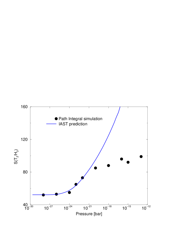
Figure 6: Finite pressure T₂/H₂ selectivity in the (2,8) tube at 20 K, assuming a bulk mole fraction of T₂ equal to $y_{T_{2}}=0.1$. Solid line, prediction from IAST theory. Circles, path integral simulations.

Also the path integral simulations show an increase of the selectivity at finite pressure, but this increase is not as steady as the IAST prediction. In fact the selectivity seems to tend to a constant value as the pressure is raised, as can be seen in Fig. 6. We notice that the correct selectivity starts to deviate from the approximate IAST value at the pressure ($10^{-21}$ bar in this case) where the adsorption isotherms begin to show saturation.

The reason of this behaviour can be traced back to the structure of the adsorbed phase. Each of the two pure species occupy the same nanotube with an almost equal linear density around $0.27$ molecules/Å. Therefore one might expect an “average distance” $L\simeq 3.7$ Å between the molecules in the case of a saturated mixture.

In going from zero to finite pressures one can then expect that the motion along the $z$ coordinate of a given molecule is progressively hindered by the ever close presence of the other ones, until a saturation condition is reached, and further compression of the system becomes more difficult.

This picture can be validated by the results reported in Fig. 7, where we plot the average center of mass kinetic energies for H₂ and T₂ as well as the average fluid-fluid energy for the mixture adsorbed in the (2,8) tube.

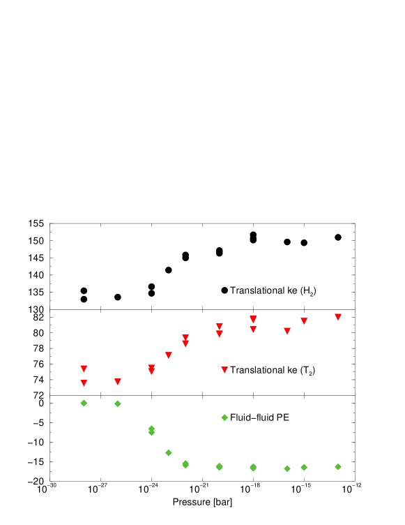
Figure 7: Average translational kinetic energy (circles, H₂; triangles, T₂) and average solid fluid potential energy (diamonds) for the adsorption of a T₂/H₂ mixture ($y_{T_{2}}=0.1$) in the (2,8) carbon nanotube at 20 K.

We notice that the average potential energy per molecule tends to a constant value of $V\simeq-16.5$ K, indicating that the molecular configuration does not change very much after the onset of saturation.

The effect of the localization along the $z$ direction is apparent from the behaviour of the kinetic energies as a function of the loading. The values for T₂ and H₂, reported in Fig. 7, do indeed show an increase at finite loading with respect to the zero pressure value. This indicates a progressive hindrance of the motion along the nanotube axis, until the saturation point is reached and the kinetic energy tends to a constant value.

It is possibile to make an estimate of these effects, by assuming that - at saturation - all the molecules in the tube are separated from their neighbors by the same distance, $L_{min}$. In order to calculate $L_{min}$ one can assume that the molecules interact with an effective potential obtained by averaging the original potential on the rotational degrees of freedom. This takes into account the fact that the (2,8) tube is wide enough so that the molecules are freely rotating. It is then possible to calculate the average potential energy per particle, $V_{FF}(x)$, as a function of the distance $x$ between the molecules, assuming that every molecule has two nearest neighbors located at $\pm x$.

The distance $L_{min}$ is then calculated as the point of mechanical equilibrium, $\partial V_{FF}(x)/\partial x=0$, obtaining the value $L_{min}=3.43$ Å, not too distant from the experimental average distance given above. In this configuration the potential energy per particle is given by $V_{FF}(L_{min})=-51.6$ K.

We further assume that any molecule performs harmonic motions around the potential energy minimum. In the actual system, of course, the dynamics is determined by anharmonic effects, so that the following estimate has only a heuristic value. The “spring constant” for these oscillation is evaluated to be $k_{HO}=\partial^{2}V_{FF}/\partial x^{2}~{}(L_{min})=316.8$ K/Ų. Hydrogen isotopes oscillating in this harmonic potential would have a zero point energy of $E_{0}^{{\rm T}_{2}}=\hbar\sqrt{k_{HO}/m_{{\rm T}_{2}}}/2=25.2$ K and $E_{0}^{{\rm H}_{2}}=43.7$ K for T₂ and H₂ respectively, so that we might expect $V>V_{FF}(L_{min})+E_{0}^{{\rm T}_{2}}=-26.4$ K, close to the actual value observed.

One can further estimate the asymptotic value of the selectivity at finite pressure by assuming the that its value at saturation is given by the product of the zero pressure value $S_{0}$ and the selectivity $S_{HO}$ due to the effective 1D harmonic oscillator discussed above. Using and independent particle approach, Wang et al. (1999); Challa et al. (2001) the value of $S_{HO}$ corresponding to T₂ and H₂ in a harmonic oscillator of spring constant $k_{HO}$ turns out to be $S_{HO}=1.6$, in reasonable agreement with the observed behavior of the selectivity which tends, at saturation, to twice the zero pressure value.

IV Conclusions

In this paper we have presented an algorithm for the hybrid path integral Monte Carlo simulation of rigid diatomic molecules. We show how to calculate torques from the expression of the rotational density matrix and we moreover show an approximate expression for the rotational density matrix of heteronuclear molecules that, in the large $P$ limit, is completely analogous to the expression for the translational degrees of freedom. We have developed a velocity Verlet like integrator for the rotational degrees of freedom suitable for a multiple time step approach.

We have then applied this method to the calculation of the para-T₂/para-H₂ selectivity in various carbon nanotubes at 20 K. We have discussed, in particular, the effect of the quantized rotational degrees of freedom on the selectivity by developing a simulation method that allows a classical treatement of the rotations while keeping a quantum tratment of the translational degrees of freedom.

We show that the explicit inclusion of quantized rotations enhances the zero pressure selectivity by a factor of more than $2000$ in the narrowest tube we have investigated (the (3,6)), but does not have such a dramatic effect in larger tubes. The rotational degrees of freedom contribute by less than a factor of two in the (2,8) and larger tubes.

We have been able to investigate the effect of finite pressures on the adsorption and the selectivity. We have calculated the adsorption isotherms of various hydrogen isotopes in different tubes at 20 K and shown that quantum effects hinder the adsorption of the lighter specie, whose isoterm can be separated by many order of magnitude in pressure from the one of the heavier specie.

We have been able to calculate pressure dependence on the selectivity on the pressure and found that, for a 0.1 molar mixture of T₂ in the (2,8) tube, the selectivity tends to twice its zero pressure value when the pressure is raised. We correlate this behaviour to the hindrance of the molecular motion along the nanotube axis.

Appendix A Velocity-Verlet integrator for rigid linear molecules

The dynamics of a rigid rotor is described by the equations

$$\frac{d{\mathbf{e}}}{dt} = {\mathbf{\varpi}}\times{\bf e}$$ (29)

$$I\frac{d{\mathbf{\varpi}}}{dt} = N$$ (30)

where ${\bf e}$ is a unit vector in the direction of the rotor and, $\varpi$ is the angular velocity, $I$ is the inertia moment and $N$ is the torque applied to the system.

These dynamical variable are redundant, since it can be seen that the norm of the vector ${\bf e}$ is a constant of the motion described by the previous equations. Since the torque $N$ is, by construction, always orthogonal to the axis vector, the component of the angular velocity along the unit vector is also a constant of motion, and is usually set as zero.

The previous equations cannot be then put in the form of a Hamiltonian system. In order to develop a time-reversible integrator that can be used in the hybrid Monte Carlo method, we demonstrate that it is indeed possibile to integrate the equations using a velocity Verlet like, adapted to take into account the abovementioned constraint. The multi-step algorithm can them be developed by analogy to the velocity Verlet case.

Using the Taylor expansion we can write

$${\bf e}(t+\delta t) \simeq {\bf e}(t)+\delta t\frac{d{\bf e}}{dt}+\frac{1}{2}(\delta t)^{2}\frac{d^{2}{\bf e}}{dt^{2}}$$ (31)

$$= {\bf e}+\delta t(\varpi\times{\bf e})+\frac{1}{2}(\delta t)^{2}\frac{d}{dt}(\varpi\times{\bf e})$$ (32)

$$= {\bf e}+\delta t(\varpi\times{\bf e}(t))+\frac{1}{2}(\delta t)^{2}\left(\frac{d\varpi}{dt}\times{\bf e}+\varpi\times(\varpi\times{\bf e})\right)$$ (33)

$$= {\bf e}(t)+\delta t\left[\left(\varpi(t)+\frac{\delta t}{2}\frac{N(t)}{I}\right)\times{\bf e}(t)\right]-\frac{(\delta t)^{2}}{2}\varpi^{2}{\bf e}(t)$$ (34)

where we have restored the explicit time dependence on time in the last passage.

The last term in Eq. (34) assures that the length of the unit vector describing the direction of the rotor remains fixed. In our code we re-normalize the unit vector after each time step.

The equation for the angular velocity becomes

$$\varpi(t+\delta t) \simeq \varpi(t)+\delta t\frac{d\varpi}{dt}+\frac{(\delta t)^{2}}{2}\frac{d^{2}\varpi}{dt^{2}}$$ (35)

$$= \varpi+\frac{\delta t}{2}\dot{\varpi}+\frac{\delta t}{2}\left(\dot{\varpi}+\delta t\ddot{\varpi}\right)$$ (36)

$$= \varpi(t)+\frac{\delta t}{2}\frac{N(t)}{I}+\frac{\delta t}{2}\frac{N(t+\delta t)}{I}$$ (37)

So that one can construct a velocity Verlet like algorithm for the rotational degrees of freedom as

1. Calculate the angular velocity at half time step $\varpi(t+\delta t/2)=\varpi(t)+\frac{\delta t}{2}\frac{N(t)}{I}$

2. Advance the orientation ${\mathbf{e}}$ at full time step, using Eq. (34)

3. Calculate the torques at the time $t+\delta t$

4. Advance the angular velocity at full time step

Appendix B Approximate treatment of the rotational density matrix

It is known to be impossible to rewrite the rotational partition function in Eq. (11) as the partition function of an effective harmonic potential, as happens for the translational degrees of freedom.

We have noticed, though, that if $P$ is large enough the rotational partition function of a heteronuclear molecule can be approximated by an expression analogous to Eq. (8) for the translational degrees of freedom.

$$\Xi_{ij}({\theta})=\sum_{J=0}^{\infty}\frac{2J+1}{4\pi}P_{J}(\cos\theta_{ij})\exp[-\beta J(J+1)B/P]\mathop{\rightarrow}_{P\rightarrow\infty}A\exp\left[-\frac{\beta K}{2}\theta^{2}_{ij}\right]$$ (38)

where

$$A = \frac{Ik_{B}TP}{2\pi\hbar^{2}}$$ (39)

$$K = \frac{IP(k_{B}T)^{2}}{\hbar^{2}}$$ (40)

Eq. (39) can be demonstrated by setting $\theta_{ij}=0$ and approximating the sum over $J$ in Eq. (11) with an integral. We have not been able to demonstrate Eq. (38) analytically, but we have verified that the first 20 coefficients of the expansion in $\theta_{ij}$ of both sides of Eq. (38) are the same in the $P\rightarrow\infty$ limit and that the exact and approximate density matrices are very similar in the same limit. We would like to point out the formal similarity between Eqs (39) and (40) and the corresponding ones for the translational degrees of freedom, Eqs. (9) and (10): in the large $P$ limit the quantum mechanical effect corresponds to the action of an harmonic torque between the rotors in adjacent time slices.

We show in Fig. 8 the difference between the numerical and the approximated rotational density matrix of Eq. (38), for HD and DT at a temperature $T=20$ K, using a Trotter number $P=100$. We can see that the approximate expression is accurate within 1.5% in the low $\theta$ region for the ligher specie. At a constant Trotter number, the approximation is of course better for a heavier molecule such as DT.

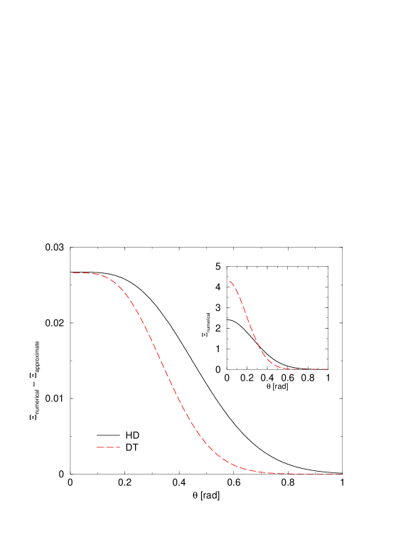
Figure 8: The difference between the approximated and the numerical rotational density matrix for HD (solid line) and DT (dashed line) at 20 K with $P=100$. The numerical density matrices for the same Trotter numbers are shown in the inset.

One can see from Eq. (38) that in the large $P$ limit the quantum rotational density matrix is analogous to the translational case (see Eq. (8)), i.e. represents an effective harmonic potential energy between adjacent beads in the classical mapping.

This is also apparent in the calculation of the torques, that we use in the hybrid Monte Carlo calculation. We report in Fig. 9 the results obtained using the numerical method derived in Eq. (19) and the analytical calculation, using the “spring constant” of Eq. (40). The two methods give virtually the same values, even though the numerical calculation shows numerical instabilities for angles just a little higher than the one shown in Fig. 9.

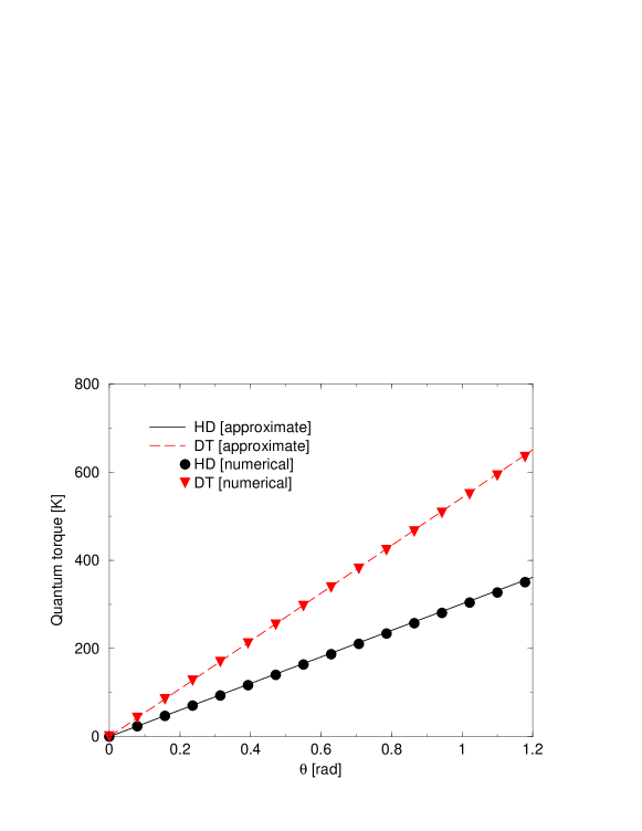
Figure 9: The quantum torque calculated numerically using Eq. (19) (symbols) and analytically using the “spring constant” given in Eq. (40) (lines). Solid line and circles refer to HD at 20K, dashed line and triangles to DT at 20K. In both cases we have set $P=100$.

Unfortunately the approximation of Eq. (38) is not applicable for ortho- and para- species, because $\Xi_{ij}(\theta)$ does not fall monotonously to zero for large $\theta$, as implied by the right hand side of Eq. (38).

If the summation in Eq. (38) is restricted to the even angular momenta only, one obtains a density matrix with the propriety $\Xi_{ij}(\pi/2+\theta)=\Xi_{ij}(\pi/2-\theta)$, such as the one shown in Fig. 10. ($\Xi_{ij}(\theta)$ would be odd with respect to the point $\theta=\pi/2$ if the odd angular momenta only were used in Eq. (38).)

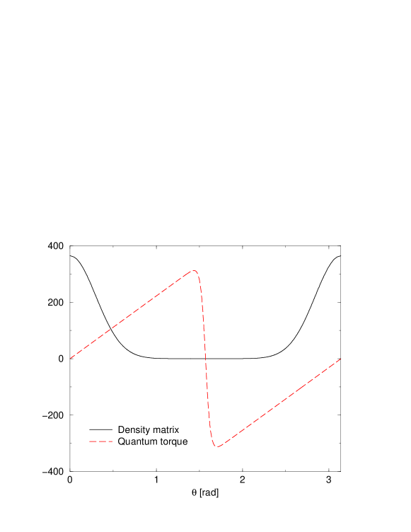
Figure 10: Density matrix (solid line) and corresponding torque (dashed line) for para-H₂ at 20K, using $P=100$.

The approximation of Eq. (38) is still valid for $\theta<\pi/2$, with the modification $A\rightarrow A/2$. Since the density matrix is even with respect to $\theta=\pi/2$, one could try to approximate it as

$$\Xi(\theta_{ij})\simeq\frac{A}{2}\exp\left[-\frac{K\theta_{ij}^{2}}{2k_{B}T}\right]\Theta(\pi/2-x)+\frac{A}{2}\exp\left[-\frac{K(\pi-\theta_{ij})^{2}}{2k_{B}T}\right]\Theta(x-\pi/2)$$

where we have denoted by $\Theta(x)$ the step function, which is 0 for $x<0$ and 1 for $x>0$. Unfortunately this will result in a discontinuous quantum torque at $\theta=\pi/2$, and we have not pursued the idea further. Nonetheless the approximate expression of Eqs. (38) – (40) may prove to be useful for an efficient quantum simulation of heteronuclear molecules, where no such discontinuities appear.

It is interesting to notice that in the classical limit $\hbar\rightarrow 0$ the torque constant of Eq. (40) goes to infinity. One could then conclude, albeit heuristically, that a classical treatment of the rotational degrees of freedom only can be done by assuming that the orientations of all the beads corresponding to one molecule all point in the same direction, in agreement with the derivation presented in Sec. II.6.

In order to test the validity of the approximation in Eq. (38), we have evaluated the zero pressure selectivity of a DT/HT mixture in the (3,6) tube using the approximate and exact method to evaluate the rotational density matrix. The results, shown in Table 2 show that the approximate method compares very well with the exact one, even if the rotational kinetic energies are sensibly different (but still within the quite large error bars) and the zero pressure selectivity of a DT/HD mixture is overestimated by 50%. In this type of calculation, which considered $N=64$ particles with $P=100$ and parallelization on 8 nodes, we have observed a 35% speedup using the approximate method.

Property	Exact result	Approximate result
Solid-fluid potential energy (K)	$-745\pm 5$	$-757\pm 5$
Translational kinetic energy (K)	$252.8\pm 0.5$	$253.2\pm 0.5$
Rotational kinetic energy (K)	$172\pm 43$	$192\pm 44$
$\langle\Delta\theta\rangle$ (degrees)	$17.5\pm 0.2$	$17.4\pm 0.2$
$R_{gyr}$ (Å)	$0.314\pm 0.008$	$0.316\pm 0.008$
$S_{0}({\rm DT}/{\rm HD})$	5450	8470

Table 2: Comparison of the approximate and exact method for the calculation of the density matrix. Properties of HD in a (3,6) carbon nanotube at 20 K with $P=100$. $\langle\Delta\theta\rangle$ is the average angle between the orientation of two adjacent beads and $R_{gyr}$ is the gyration radius of the classical ring polymer.

References

- Katorski and White (1964) A. Katorski and D. White, J. Chem. Phys. 40, 3183 (1964).
- Moiseyev (1975) N. Moiseyev, J. Chem. Soc. Faraday Trans. 1 71, 1830 (1975).
- Beenakker et al. (1995) J. Beenakker, V. Borman, and S. Krylov, Chem. Phys. Lett. 232, 379 (1995).
- Wang et al. (1999) Q. Wang, S. Challa, D. Sholl, and J. Johnson, Phys. Rev. Lett. 82, 956 (1999).
- Challa et al. (2001) S. Challa, D. Sholl, and J. Johnson, Phys. Rev. B 63, 245419 (2001).
- Challa et al. (2002) S. Challa, D. Sholl, and J. Johnson, J. Chem. Phys. 116, 814 (2002).
- Hathorn et al. (2001) B. Hathorn, B. Sumpter, and D. Noid, Phys. Rev. A 64, 022903 (2001).
- Trasca et al. (2003) R. Trasca, M. Kostov, and M. Cole, Phys. Rev. B 67, 035410 (2003).
- Lu et al. (2003) T. Lu, E. Goldfield, and S. Gray, J. Phys. Chem. B 107, 12989 (2003).
- Garberoglio et al. (2006) G. Garberoglio, M. DeKlavon, and J. Johnson, J. Phys. Chem. B 110, 1733 (2006).
- Lu et al. (2006) T. Lu, E. Goldfield, and S. Gray, J. Phys. Chem. B 110, 1742 (2006).
- Landau and Binder (2000) D. Landau and K. Binder, A guide to Monte Carlo simulations in statistical physics (Cambridge University Press, 2000), chap. 8.
- Marx and Müser (1999) D. Marx and M. Müser, J. Phys.: Condens. Matter 11, R117 (1999).
- Cui et al. (1997) T. Cui, E. Cheng, B. Adler, and K. Whaley, Phys. Rev. B 55, 12253 (1997).
- Duane et al. (1987) S. Duane, A. Kennedy, B. Pendleton, and D. Roweth, Phys. Lett. B 195, 216 (1987).
- Tuckerman et al. (1993) M. Tuckerman, B. Berne, G. Martyna, and M. Klein, J. Chem. Phys. 99, 2796 (1993).
- Tuckerman et al. (1992) M. Tuckerman, B. Berne, and G. Martyna, J. Chem. Phys. 97, 1990 (1992).
- Matubayasi and Nakahara (1999) N. Matubayasi and M. Nakahara, J. Chem. Phys. 110, 3291 (1999).
- Wang et al. (1997) Q. Wang, J. Johnson, and J. Broughton, J. Chem. Phys. 107, 5108 (1997).
- Murad and Gubbins (1978) S. Murad and K. Gubbins, in Computer Modelling of Matter (American Chemical Society, Washington, 1978), vol. 86 of ACS Symposium series, p. 62.
- Steele (1978) W. Steele, J. Phys. Chem. 82, 817 (1978).