Non-Perturbative Treatment of Charge and Spin Fluctuations in the Two-Dimensional Extended Hubbard Model: Extended Two-Particle Self-Consistent Approach

Abstract

We study the spin and charge fluctuations of the extended Hubbard model (EHM) with on-site interaction $U$ and first neighbor interaction $V$ on the two-dimensional square lattice in the weak to intermediate coupling regime. We propose an extension of the two-particle self-consistent (ETPSC) approximation that includes the effect of functional derivatives of the pair correlation functions on irreducible spin and charge vertices. These functional derivatives were ignored in our previous work. We evaluate them assuming particle-hole symmetry. The resulting theory satisfies conservations laws and the Mermin-Wagner theorem. Our current results are in much better agreement with benchmark Quantum Monte-Carlo (QMC) results. As a function of $U$ and $V,$ we can determine the crossover temperatures towards renormalized classical regimes where either spin or charge fluctuations dominate. The dominant wave vector is self-determined by the approach.

I Introduction

The single-band Hubbard model, with on-site interaction $U$ and nearest-neighbor hopping $t,$ is the simplest model of correlated electrons. It has been extensively studied, for example, in the context of high-temperature superconductors. Charge ordering phenomena in strongly correlated systems are also quite common, for example in manganites, vanadates, cobaltates and various organic conductors. Imada:2005 ; Oles In these cases, and even in high temperature superconductors where screening is not perfect, it is useful to investigate the Extended Hubbard model (EHM) that includes the effect of nearest-neighbor Coulomb repulsion $V$. In that model, charge and spin fluctuations compete over much of the phase diagram.

Even at weak to intermediate coupling, $\left(U\text{ and }V\text{ less than the bandwidth }W=8t\text{ in }d=2\right)$ very few many-body methods can treat the Hubbard model while adequately taking into account the Mermin-Wagner theorem. The Fluctuation-Exchange Approximation (FLEX) Bickers:1989 is such a method. The Two-Particle Self-Consistent approach (TPSC) Vilk1 ; Vilk2 ; Mahan ; Hankevych is an alternate non-perturbative approach that compares much better with benchmark Quantum Monte Carlo (QMC) simulations. In addition, contrary to FLEX, it reproduces the pseudogap phenomenon observed in QMC. Moukouri ; AllenKyung

In this paper, we present an extension of the TPSC approach that allows one to treat the EHM. The accuracy of the new approach is checked by comparing with QMC simulations. Zhang The competition between charge and spin fluctuations in parameter space is also explored for two fillings. Whenever possible we compare with results of other approaches available in the literature. Studies for the specific parameters appropriate for given compounds will be the subject of separate papers. The purpose of the present one is to give a detailed description of the theoretical approach, which is an extension of the TPSC approach.

Briefly speaking, the TPSC method was derived from a functional approach by approximating the vertex functions as local functions of the imaginary time and space (in other words irreducible vertices independent of frequency and wave vector). This leads to irreducible spin and charge vertices that contain two unknown constants, namely the on-site pair correlation function and its functional derivative, which can be self-consistently determined from two sum-rules on the structure functions. Unfortunately the number of unknowns becomes more than the number of available sum-rules in the EHM, so one has to use another approach. In our previous work, Bahman we simply neglected the contribution of functional derivatives of the pair correlation functions. We obtained good agreement with QMC results for small values of $V$ when spin fluctuations are still dominant, but this approach did not work so well in the opposite limit when charge fluctuations becomes dominant. This is mainly due to ignoring the functional derivative of the pair correlation functions. In this paper, we demonstrate the importance of these functional derivative terms, explain the way they enter in the formalism and propose a way to use particle-hole symmetry to evaluate them.

The EHM has been studied within different approaches and approximations. We can only give a sample of the literature. Many papers focus on the quarter-filled case on the square lattice or on ladders Seo:1998 ; Pietig:1999 ; Vojta:1999 ; Hellberg:2001 ; Vojta:2001 ; Hoang:2002 ; Calandra:2002 ; Imada:2005 . The competition between charge and spin orders has also been studied in other dimension: one- Fourcade ; Bosch:1988 ; Aichhorn:2004 , three- Barktowiak:1995 and higher dimensions VanDongen:1994 at various fillings. In two dimensions, there are several studies at strong coupling Avella:2004 ; Avella:2006 ; Vojta:2002 or on lattices different from the square lattice. Kuroki:2006 ; Seo:2006 The combined effect of charge fluctuations in addition to the usual spin fluctuation in favouring one type or another of unconventional superconductivity has also been studied using this model Onari ; Kishine:1995 ; Callaway:1990 ; Scalapino ; Esirgen .

On the two-dimensional square lattice, QMC studies Zhang will be particularly relevant as mentioned above. We have not found any systematic comparison between FLEX approximation for the EHM Onari and QMC. The mean field (MF) approximation Yan:2006 and the renormalization group (RG) approach Murakami , as well as exact diagonalization Ohta:1994 , perturbation theory about ordered states Yan:1993 and trial correlated wave functions Oles have been applied to this problem. One of the results that we will find at half-filling is a crossover line at $U\approx 4V$ from dominant antiferromagnetic fluctuations to dominant checkerboard charge fluctuations. This is in agreement with several studies Zhang ; Onari ; Oles ; Ohta:1994 ; Yan:1993 ; Bari:1971 as we will discuss. Our results hold at the crossover temperature. Most other approaches focus on the ground state. The result $U=zV,$ where $z$ is the number of nearest-neighbors, seems to hold quite generally in various dimensions. Oles ; Fourcade ; Micnas Some MF results Murakami give the possibility of a coexistence region between charge and spin density waves. The Pauli principle prevents charge and spin fluctuations to increase at the same time in the paramagnetic regime at finite temperature. This is satisfied within our approach.

In the following we present the formalism, which first focuses on finding a set of closed equations for the irreducible vertices. We explain how the functional derivative of the pair correlation functions enter in the evaluation of irreducible vertices. In the second part of the theory section, we explain how particle-hole symmetry can be used to estimate the functional derivatives and we give the details of the new resulting Extended TPSC (ETPSC) approach. In Sec. III, we present numerical results and compare them with available QMC results to gauge the accuracy of the approach. The last part of that section presents a systematic study on the square lattice of the crossover to the renormalized classical regimes for charge and spin fluctuations for two densities, $n=1$ and $n=0.75$. Finally, in the concluding section we discuss the possibility to use the same type of approximation for other systems and point towards possible future developments and improvements.

II Theory

II.1 Some exact results, factorization and approximation for the functional derivatives

The extended Hubbard Hamiltonian is defined by,

$$H = -t\sum_{\left\langle\mathbf{ij}\right\rangle\sigma}(c_{\mathbf{i}\sigma}^{\dagger}c_{\mathbf{j}\sigma}+c_{\mathbf{j}\sigma}^{\dagger}c_{\mathbf{i}\sigma})+U\sum_{\mathbf{i}}n_{\mathbf{i}\uparrow}n_{\mathbf{i}\downarrow}$$ (2)

$$+V\sum_{\left\langle\mathbf{ij}\right\rangle\sigma\sigma^{\prime}}n_{\mathbf{i}\sigma}n_{\mathbf{j}\sigma^{\prime}}-\mu\sum_{\mathbf{i}}n_{i}$$

where $c_{\mathbf{i}\sigma}$ ($c_{\mathbf{i}\sigma}^{\dagger}$) are annihilation (creation) operators for an electron with spin $\sigma$ in the Wannier orbital at site $i$, $n_{\mathbf{i}\sigma}=c_{\mathbf{i}\sigma}^{\dagger}c_{\mathbf{i}\sigma}$ is the density operator for electrons of spin $\sigma$, $t$ is the hopping matrix element and $\mu$ is the chemical potential. The terms proportional to $U$ and $V$ represent respectively the on-site and nearest-neighbor interactions. The latter $\left(V\right)$ vanishes for the usual Hubbard model.

To generalize the TPSC approach, we use the same formalism as in Ref. Allen:2003, . The Green function is defined by

$$G_{\sigma}(1,2) = -\frac{\delta\ln Z[\phi_{\sigma}]}{\delta\phi_{\sigma}(2,1)}=-\left\langle T_{\tau}c_{1\sigma}(\tau_{1})c_{2\sigma}^{\dagger}(\tau_{2})\right\rangle$$ (3)

$$= -\left\langle T_{\tau}c_{\sigma}(1)c_{\sigma}^{\dagger}(2)\right\rangle$$ (4)

where the brackets $\left\langle{}\right\rangle$ represents a thermal average in the canonical ensemble, $T_{\tau}$ is the time-ordering operator, and $\tau$ is the imaginary time. The space and imaginary time coordinates $\left(\mathbf{r}_{1},\tau_{1}\right)$ are abbreviated as $\left(1\right).$ The generating functional $Z[\phi_{\sigma}]$ is given by

$$Z[\phi_{\sigma}]=\mathrm{Tr}\left[e^{-\beta H}T_{\tau}S(\beta)\right]$$ (5)

and $S(\beta)$ is defined as follows

$$\ln S(\beta)=-\sum_{\mathbf{i},\mathbf{j},\sigma}\int_{0}^{\beta}d\tau d\tau^{\prime}c_{\mathbf{i}\sigma}^{\dagger}(\tau)c_{\mathbf{j}\sigma}(\tau^{\prime})\phi_{\sigma}(\mathbf{i},\mathbf{j},\tau,\tau^{\prime}).$$ (6)

The equation of motion for the Green function takes the form of the Dyson equation BaymKadanoff:1962 ; Vilk2

$$G_{\sigma}^{-1}(1,2)=G_{0}^{-1}(1,2)-\phi_{\sigma}(1,2)-\Sigma_{\sigma}(1,2).$$ (7)

The expression for $\Sigma G$ comes from the commutator with the interaction part of the Hamiltonian so that the self-energy in the above equation is given by

$$\Sigma_{\sigma}(1,2)=-U\left\langle T_{\tau}c_{\tilde{\sigma}}^{\dagger}(1)c_{\tilde{\sigma}}(1)c_{\sigma}(1)c_{\sigma}^{\dagger}(\bar{3})\right\rangle G_{\sigma}^{-1}(\bar{3},2)-V\sum_{\sigma^{\prime},a}\left\langle T_{\tau}c_{\sigma^{\prime}}^{\dagger}(1+a)c_{\sigma^{\prime}}(1+a)c_{\sigma}(1)c_{\sigma}^{\dagger}(\bar{3}),\right\rangle G_{\sigma}^{-1}(\bar{3},2)$$ (8)

where $\tilde{\sigma}=-\sigma$ and the summation on $a$ runs over the next neighbor sites of the site $1$ (at the same imaginary time).

The first approximation is inspired by TPSC. We factorize the two-body density matrix operators as follows, defining numbers with overbars, such as $\bar{3},$ to mean a sum over the corresponding spatial indices and integration over the corresponding imaginary time:

$$\Sigma_{\sigma}(1,2) \cong UG_{\tilde{\sigma}}(1,1^{+})G_{\sigma}(1,\bar{3})G_{\sigma}^{-1}(\bar{3},2)g_{\sigma\tilde{\sigma}}(1,1)+V\sum_{\sigma^{\prime},a}G_{\sigma^{\prime}}(1+a,1+a^{+})G_{\sigma}(1,\bar{3})G_{\sigma}^{-1}(\bar{3},2)g_{\sigma\sigma^{\prime}}(1,1+a)$$

$$=U\delta(1,2)G_{\tilde{\sigma}}(1,1^{+})g_{\sigma\tilde{\sigma}}(1,1)+V\delta(1,2)\sum_{\sigma^{\prime},a}G_{\sigma^{\prime}}(1+a,1+a^{+})g_{\sigma\sigma^{\prime}}(1,1+a).$$ (9)

If we set $g_{\sigma\sigma^{\prime}}(i,j)=1$ in the above expression, one recovers the Hartree-Fock approximation for the $U$ term, and the Hartree approximation for the $V$ term. The Fock term in the near neighbor interaction $V$ leads to a renormalization of the band parameters and is not as essential as in the on-site term, as discussed in our previous paper.Bahman The above expression for the self-energy goes beyond the Hartree-Fock approximation because of the presence of the pair correlation functions $g_{\sigma\sigma^{\prime}}(i,j)$ defined by

$$g_{\sigma\sigma^{\prime}}(1,2)\equiv\frac{\left\langle n_{\sigma}\left(1\right)n_{\sigma^{\prime}}\left(2\right)\right\rangle-\delta(1,2)\delta_{\sigma,\sigma^{\prime}}\left\langle n_{\sigma}\left(1\right)\right\rangle}{\left\langle n_{\sigma}\left(1\right)\right\rangle\left\langle n_{\sigma^{\prime}}\left(2\right)\right\rangle}.$$ (10)

This quantity is related to the probability of finding one electron with spin $\sigma^{\prime}$ on site $j$ when another electron with spin $\sigma$ is held on site $i$. The presence of the pair correlation function is analog to the local field correction in the Singwi approach to the electron gas. Singwi Thanks to this correction factor, we recover the exact result that the combination $\Sigma_{\sigma}(1,\bar{3})G_{\sigma}(\bar{3},2)$ is equal to the potential energy when point $2$ becomes $1^{+}$ (where the superscript $+$ refers to the imaginary time and serves to order the corresponding field operator to the left of operators at point $1$). For this special case then, $g_{\sigma\sigma^{\prime}}(1,1+a)$ contains the information about the Fock contribution as well.

We need the response functions obtained from the first functional derivative of the Green function with respect to the external field. Taking the functional derivative of the identity $G_{\sigma}(1,\bar{3})G_{\sigma^{\prime}}^{-1}(\bar{3},2)=\delta_{\sigma\sigma^{\prime}}\delta(1,2)$ and using Dyson’s equation Eq. (7), we find

$$\chi_{\sigma\sigma^{\prime}}(1,2;3,3) \equiv-\frac{\delta G_{\sigma}(1,2)}{\delta\phi_{\sigma^{\prime}}(3,3)}=G_{\sigma}(1,\bar{4})\frac{\delta G_{\sigma}^{-1}(\bar{4},\bar{5})}{\delta\phi_{\sigma^{\prime}}(3,3)}G_{\sigma}(\bar{5},2)$$

$$=-\delta_{\sigma\sigma^{\prime}}G_{\sigma}(1,3)G_{\sigma}(3,2)-\sum_{\sigma^{\prime\prime}}G_{\sigma}(1,\bar{4})\frac{\delta\Sigma_{\sigma}(\bar{4},\bar{5})}{\delta G_{\sigma^{\prime\prime}}(\bar{6},\bar{7})}\frac{\delta G_{\sigma^{\prime\prime}}(\bar{6},\bar{7})}{\delta\phi_{\sigma^{\prime}}(3,3)}G_{\sigma}(\bar{5},2).$$ (11)

The irreducible vertex is the first functional derivative of the self-energy respect to the Green function, as can be seen from the last equation. It can be obtained from our equation for the self-energy Eq. (9):

$$\frac{\delta\Sigma_{\sigma}(4,5)}{\delta G_{\sigma^{\prime\prime}}(6,7)} =U\delta_{\tilde{\sigma}\sigma^{\prime\prime}}\delta(4,5)\delta(4,6)\delta(5,7)g_{\sigma\tilde{\sigma}}(4,4)+V\sum_{a}\delta(4,5)\delta(4+a,6)\delta(5+a,7)g_{\sigma\sigma^{\prime\prime}}(4,4+a)$$

$$+U\delta(4,5)G_{\tilde{\sigma}}(4,4^{+})\frac{\delta g_{\sigma\tilde{\sigma}}(4,4)}{\delta G_{\sigma^{\prime\prime}}(6,7)}+V\delta(4,5)\sum_{\sigma^{\prime\prime\prime},a}G_{\sigma^{\prime\prime\prime}}(4,4^{+})\frac{\delta g_{\sigma\sigma^{\prime\prime\prime}}(4,4+a)}{\delta G_{\sigma^{\prime\prime}}(6,7)}.$$ (12)

In the standard Hubbard model with $V=0$, there is only one unknown functional derivative of the pair correlation function with respect to the Green function. Since it enters only the charge response function , it can be determined by making the local approximation, enforcing the Pauli principle and requiring that the fluctuation-dissipation theorem relating charge susceptibility to pair correlation function be satisfied. Vilk2 In the present case, there are not enough sum rules to determine the additional functional derivatives of the pair correlation functions with respect to the Green function.

In our previous paper on the extended Hubbard model, Bahman we neglected these additional unknown functional derivatives. Here we present an approximation for these functional derivatives that improves our previous results, as can be judged by comparisons with QMC calculations. We would like to replace the unknown terms by functional derivatives with respect to the density as $\frac{\delta g_{\sigma\sigma^{\prime}}(1,2)}{\delta G_{\sigma^{\prime\prime}}(3,4)}\approx\frac{\delta g_{\sigma\sigma^{\prime}}(1,2)}{\delta n_{\sigma^{\prime\prime}}(3)}\delta(3,4)$. Unfortunately we cannot evaluate this type of functional derivative either, unless point $3\$coincides with either $2$ or $1$, so we approximate the previous equation by

$$\frac{\delta g_{\sigma\sigma^{\prime}}(1,2)}{\delta n_{\sigma^{\prime\prime}}(3)}\approx\frac{\delta g_{\sigma\sigma^{\prime}}(1,2)}{\delta n_{\sigma^{\prime\prime}}(1)}\delta(1,3)+\frac{\delta g_{\sigma\sigma^{\prime}}(1,2)}{\delta n_{\sigma^{\prime\prime}}(2)}\delta(2,3).$$ (13)

In other words, we ignore the terms where point $3$ gets further away from either $1$ or $2$. We will show that the last equation is exact at half-filling (see Eq.(30)) and that it can be evaluated . We will also show in the next section by explicit comparisons with QMC calculations that its extension away from half-filling is a reasonable approximation. The last two approximations lead to the local approximation of TPSC as a special case.

Inserting in the susceptibility Eq. (II.1) the irreducible vertex obtained from Eq. (II.1) and our approximation for the functional derivatives, we find

$$\chi_{\sigma\sigma^{\prime}}(1;2)= -\delta_{\sigma\sigma^{\prime}}G_{\sigma}(1,2)G_{\sigma}(2,1)$$

$$-UG_{\sigma}(1,\bar{3})G_{\sigma}(\bar{3},1)g_{\sigma\tilde{\sigma}}(\bar{3},\bar{3})\frac{\delta G_{\tilde{\sigma}}(\bar{3},\bar{3}^{+})}{\delta\phi_{\sigma^{\prime}}(2,2)}$$

$$-VG_{\sigma}(1,\bar{3})G_{\sigma}(\bar{3},1)\sum_{\sigma^{\prime\prime},a}g_{\sigma\sigma^{\prime\prime}}(\bar{3},\bar{3}+a)\frac{\delta G_{\sigma^{\prime\prime}}(\bar{3}+a,\bar{3}+a^{+})}{\delta\phi_{\sigma^{\prime}}(2,2)}$$

$$-UG_{\sigma}(1,\bar{3})G_{\sigma}(\bar{3},1)n_{\tilde{\sigma}}(\bar{3})\sum_{\sigma^{\prime\prime}}\frac{\delta g_{\sigma\tilde{\sigma}}(\bar{3},\bar{3})}{\delta n_{\sigma^{\prime\prime}}(\bar{3})}\frac{\delta G_{\sigma^{\prime\prime}}(\bar{3},\bar{3}^{+})}{\delta\phi_{\sigma^{\prime}}(2,2)}$$

$$-VG_{\sigma}(1,\bar{3})G_{\sigma}(\bar{3},1)\sum_{\sigma^{\prime\prime}\sigma^{\prime\prime\prime}a}n_{\sigma^{\prime\prime\prime}}(\bar{3})\left[\frac{\delta g_{\sigma\sigma^{\prime\prime\prime}}(\bar{3},\bar{3}+a)}{\delta n_{\sigma^{\prime\prime}}(\bar{3})}\frac{\delta G_{\sigma^{\prime\prime}}(\bar{3},\bar{3}^{+})}{\delta\phi_{\sigma^{\prime}}(2,2)}+\frac{\delta g_{\sigma\sigma^{\prime\prime\prime}}(\bar{3},\bar{3}+a)}{\delta n_{\sigma^{\prime\prime}}(\bar{3}+a)}\frac{\delta G_{\sigma^{\prime\prime}}(\bar{3}+a,\bar{3}+a^{+})}{\delta\phi_{\sigma^{\prime}}(2,2)}\right].$$ (14)

For the repulsive case, we expect that spin and charge components of the response functions will be dominant. Thus we need the dynamic correlation functions of the density $n=n_{\uparrow}+n_{\downarrow}$ and magnetization $m=n_{\uparrow}-n_{\downarrow}$ respectively. They are given by

$$\chi_{cc,ss}(1;2)= 2\left[\chi_{\sigma\sigma}(1;2)\pm\chi_{\sigma\tilde{\sigma}}(1;2)\right]$$

$$= -2G_{\sigma}(1,2)G_{\sigma}(2,1)$$

$$-2UG_{\sigma}(1,\bar{3})G_{\sigma}(\bar{3},1)g_{\sigma\tilde{\sigma}}(\bar{3},\bar{3})\left[\frac{\delta G_{\sigma}(\bar{3},\bar{3}^{+})}{\delta\phi_{\tilde{\sigma}}(2,2)}\pm\frac{\delta G_{\sigma}(\bar{3},\bar{3}^{+})}{\delta\phi_{\sigma}(2,2)}\right]$$

$$-4VG_{\sigma}(1,\bar{3})G_{\sigma}(\bar{3},1)\sum_{a}g_{cc,ss}(\bar{3},\bar{3}+a)\left[\frac{\delta G_{\sigma}(\bar{3}+a,\bar{3}+a^{+})}{\delta\phi_{\tilde{\sigma}}(2,2)}\pm\frac{\delta G_{\sigma}(\bar{3}+a,\bar{3}+a^{+})}{\delta\phi_{\sigma}(2,2)}\right]$$

$$-2nUG_{\sigma}(1,\bar{3})G_{\sigma}(\bar{3},1)\left\{\frac{\delta g_{\sigma\tilde{\sigma}}(\bar{3},\bar{3})}{\delta n(\bar{3})},\frac{\delta g_{\sigma\tilde{\sigma}}(\bar{3},\bar{3})}{\delta m(\bar{3})}\right\}\left[\frac{\delta G_{\sigma}(\bar{3},\bar{3}^{+})}{\delta\phi_{\tilde{\sigma}}(2,2)}\pm\frac{\delta G_{\sigma}(\bar{3},\bar{3}^{+})}{\delta\phi_{\sigma}(2,2)}\right]$$

$$-4nVG_{\sigma}(1,\bar{3})G_{\sigma}(\bar{3},1)\sum_{a}\left\{\frac{\delta g_{s\sigma}(\bar{3},\bar{3}+a)}{\delta n(\bar{3})},\frac{\delta g_{s\sigma}(\bar{3},\bar{3}+a)}{\delta m(\bar{3})}\right\}\left[\frac{\delta G_{\sigma}(\bar{3},\bar{3}^{+})}{\delta\phi_{\tilde{\sigma}}(2,2)}\pm\frac{\delta G_{\sigma}(\bar{3},\bar{3}^{+})}{\delta\phi_{\sigma}(2,2)}\right]$$

$$-4nVG_{\sigma}(1,\bar{3})G_{\sigma}(\bar{3},1)\sum_{a}\left\{\frac{\delta g_{s\sigma}(\bar{3},\bar{3}+a)}{\delta n(\bar{3}+a)},\frac{\delta g_{s\sigma}(\bar{3},\bar{3}+a)}{\delta m(\bar{3+a})}\right\}\left[\frac{\delta G_{\sigma}(\bar{3}+a,\bar{3}+a^{+})}{\delta\phi_{\tilde{\sigma}}(2,2)}\pm\frac{\delta G_{\sigma}(\bar{3}+a,\bar{3}+a^{+})}{\delta\phi_{\sigma}(2,2)}\right]$$ (15)

where the first term $A$ in the curly brackets $\left\{A,B\right\}$ is associated with the upper $+$ sign, and the second term $B$ is associated with the $-$ sign. Also, in the above equation,

$$g_{cc,ss}=(g_{\sigma\sigma}\pm g_{\sigma\tilde{\sigma}})/2$$

are the charge and spin correlation functions, while

$$g_{s\sigma}=(g_{\sigma\sigma}+g_{\sigma\tilde{\sigma}})/2$$

is the symmetric combination of the spin-resolved pair correlation functions. Indeed, the definition of $g_{cc}$ in partially spin polarized system is different from the above equation and that is the reason for defining $g_{s\sigma}$. In fact $g_{cc}$ is symmetric function under a flip of the spins of the electrons but not $g_{s\sigma}$. This is an important issue when we deal with the functional derivative of the pair correlation functions with respect to the magnetization. The functional derivative terms with respect to magnetization in the fourth and the last term are zero . This is due to the fact that $g_{\sigma\tilde{\sigma}}(1,1)$ and $g_{s\sigma}(1,2)$ are even functions under exchange of $\sigma\leftrightarrow\tilde{\sigma}$ on site $1$ and on site $2$ respectively. The functional derivative with respect to density in the fifth and last term are equal (this can also be shown by following the procedure that we explain in the following subsection). Now we can factorize the charge and spin response functions from the above equation. The final form of the response functions in Fourier-Matsubara space are given by

$$\chi_{cc}(\mathbf{q},\omega_{n})=\frac{\chi^{0}(\mathbf{q},\omega_{n})}{1+\frac{\chi^{0}(\mathbf{q},\omega_{n})}{2}U_{cc}(\mathbf{q})},$$ (16)

$$\chi_{ss}(\mathbf{q},\omega_{n})=\frac{\chi^{0}(\mathbf{q},\omega_{n})}{1-\frac{\chi^{0}(\mathbf{q},\omega_{n}))}{2}U_{ss}(\mathbf{q})},$$ (17)

where

$$U_{cc}(\mathbf{q}) =U\left(g_{\sigma\tilde{\sigma}}(1,1)+n\frac{\delta g_{\sigma\tilde{\sigma}}(1,1)}{\delta n(1)}\right)+4V\left(g_{cc}(1,1+a)\gamma(\mathbf{q})+n\frac{\delta g_{s\sigma}(1,1+a)}{\delta n(1)}(2+\gamma(\mathbf{q}))\right),$$ (18)

$$U_{ss}(\mathbf{q}) =Ug_{\sigma\tilde{\sigma}}(1,1)-4V\left(g_{ss}(1,1+a)\gamma(\mathbf{q})+2n\frac{\delta g_{s\sigma}(1,1+a)}{\delta m(1)}\right).$$ (19)

In this equation, $\gamma(\mathbf{q})$ is given by $\gamma(\mathbf{q})=\sum_{\alpha}\cos(q_{\alpha}a)$, $\alpha=1..D$, $D$ being the dimension of the system, $\omega_{n}=2\pi nT$ is the Matsubara frequency and $\chi^{0}(\mathbf{q},\omega_{n})$ is the free response function

$$\chi^{0}(\mathbf{q},\omega_{n})=\int_{BZ}\frac{d\mathbf{p}}{\nu}\frac{f^{0}(\mathbf{p}+\frac{\mathbf{q}}{2})-f^{0}(\mathbf{p}-\frac{\mathbf{q}}{2})}{i\omega_{n}-\epsilon_{\mathbf{p}+\mathbf{q}/2}+\epsilon_{\mathbf{p}-\mathbf{q}/2}}.$$ (20)

In the above formula $\nu$ is the volume of the Brillouin zone (BZ), $f^{0}(\mathbf{q})=1/[1+\exp((\epsilon_{q}-\mu)/T)]$ is the free momentum distribution function and $\epsilon_{q}=-2t\sum_{\alpha}\cos(q_{\alpha}a)$ is the free particle dispersion relation. The pair correlation functions are related to the instantaneous structure factors by

$$g_{cc}(\mathbf{r}_{\mathbf{i}})=1+\frac{1}{n}\int_{BZ}\frac{d\mathbf{q}}{\nu}[S_{cc}(\mathbf{q})-1]\exp(i\mathbf{q}\cdot\mathbf{r}_{\mathbf{i}})$$ (21)

$$g_{ss}(\mathbf{r}_{\mathbf{i}})=\frac{1}{n}\int_{BZ}\frac{d\mathbf{q}}{\nu}[S_{ss}(\mathbf{q})-1]\exp(i\mathbf{q}\cdot\mathbf{r}_{\mathbf{i}})$$ (22)

where $S_{cc,ss}(\mathbf{q})=S_{\sigma\sigma}(\mathbf{q})\pm S_{\sigma\tilde{\sigma}}(\mathbf{q})$ are the charge and spin component of the instantaneous structure factor, the spin resolved instantaneous structure factor being defined by $S_{\sigma\sigma^{\prime}}(\mathbf{q})=\left\langle n_{\sigma}(\mathbf{q})n_{\sigma^{\prime}}(\mathbf{q})\right\rangle/n$ with $n_{\sigma}(\mathbf{q})$ the Fourier transform of $n_{\mathbf{i}\sigma}$. Finally, the instantaneous structure factors are connected to the response functions (or susceptibilities) by the fluctuation-dissipation theorem

$$S_{cc,ss}(\mathbf{q})=-\frac{T}{n}\sum_{\omega_{n}}\chi_{cc,ss}(\mathbf{q},\omega_{n})$$ (23)

II.2 Particle-hole symmetry for the functional derivatives

We are left with the evaluation of the functional derivatives. We first use the particle-hole (Lieb-Mattis) canonical transformation $c_{\sigma}(i)=\exp(i\mathbf{Q}\cdot\mathbf{r}_{i})c^{\prime}{}_{{\sigma}}^{\dagger}(i)$ (where $\mathbf{Q}=(\pi,\pi)$) in the definition of the pair correlation function. In the second step we will use electron-hole symmetry to evaluate the functional derivative of the pair correlation function at half-filling. First step: When point $1\$and point $2$ are different or when $\sigma\neq\sigma^{\prime}$ the particle-hole transformation gives

$$g_{\sigma\sigma^{\prime}}(1,2)=\frac{\left\langle n_{\sigma}(1)n_{\sigma^{\prime}}(2)\right\rangle}{n_{\sigma}(1)n_{\sigma^{\prime}}(2)}=\frac{\left\langle[1-n_{\sigma}^{\prime}(1)][1-n_{\sigma^{\prime}}^{\prime}(2)]\right\rangle}{[1-n_{\sigma}^{\prime}(1)][1-n_{\sigma^{\prime}}^{\prime}(2)]}=\frac{1-n_{\sigma}^{\prime}(1)-n_{\sigma^{\prime}}^{\prime}(2)+n_{\sigma}^{\prime}(1)n_{\sigma^{\prime}}^{\prime}(2)g_{\sigma\sigma^{\prime}}^{\prime}(1,2)}{1-n_{\sigma}^{\prime}(1)-n_{\sigma^{\prime}}^{\prime}(2)+n_{\sigma}^{\prime}(1)n_{\sigma^{\prime}}^{\prime}(2)}$$ (24)

where $g^{\prime}$ is the pair correlation function of holes at the density $n^{\prime}$. Note that $n$ inside the angle brackets are the operator densities. We abbreviate average densities such as $\left\langle n_{\sigma}(1)\right\rangle$ by $n_{\sigma}(1)$.

The above equation may look innocuous, but it leads to a very strong constraint on the pair correlation function and it can be used to find the exact functional derivative of the pair correlation function at half-filling where particle-hole symmetry is exact. To obtain this we first take $n(1)=1+\epsilon$ and $m(1)=0$ which means $n^{\prime}(1)=1-\epsilon$ and $m^{\prime}(1)=0$. Note that $n\left(2\right)$ is unchanged. Using the fact that $n_{\uparrow,\downarrow}(i)=[n(i)\pm m(i)]/2$ one obtains

$$g_{\uparrow\sigma}(1,2)=\frac{\frac{\epsilon}{2}+\frac{1-\epsilon}{4}g_{\uparrow\sigma}^{\prime}(1,2)}{\frac{1+\epsilon}{4}}.$$ (25)

When there is exact electron-hole symmetry, such as at half-filling, the electron pair correlation function at density $n$ is equal to the hole pair correlation function at the same density, so we deduce from the above equation that

$$\frac{\delta g_{\uparrow\sigma}(1,2)}{\delta n(1)}=[1-g_{\uparrow\sigma}(1,2)].$$ (26)

The summation of last equation for two different values of $\sigma$ gives us one of the functional derivatives

$$\frac{\delta g_{s\sigma}(1,2)}{\delta n(1)}=[1-g_{cc}(1,2)].$$ (27)

Using the same trick we can also show that

$$\frac{\delta g_{\uparrow\downarrow}(1,1)}{\delta n(1)}=2[1-g_{\uparrow\downarrow}(1,1)].$$ (28)

To evaluate the functional derivative respect to magnetization, it suffices to assume that $n(1)=1$ and $m(1)=\epsilon$ . It is then easy to show that

$$\frac{\delta g_{s\sigma}(1,2)}{\delta m(1)}=[1-g_{cc}(1,2)].$$ (29)

Using the same trick one can also show, as mentioned before, that at half filling

$$\frac{\delta g_{\sigma\sigma^{\prime}}(1,2)}{\delta(n,m)(3)}=0$$ (30)

when site $3$ is different from both $1\;$and$\;2$. Although there is no strict particle-hole symmetry away from half-filling, it is reasonable to assume that at weak to intermediate coupling the Pauli principle forces only electrons close to the Fermi surface to be relevant. In that case, the dispersion relation can be linearized and particle-hole symmetry can be safely assumed for the pair correlation functions $g_{\sigma\sigma^{\prime}}(i,j).$ The comparisons with QMC calculations presented later suggest that it is indeed a good approximation.

II.3 Self-consistency and discussion of Extended Two-Particle Self-Consistent Approach (ETPSC)

Substituting the above equations for the functional derivatives in the expression for the irreducible vertices $U_{cc}\left(\mathbf{q}\right),$ Eq.(18), and $U_{ss}\left(\mathbf{q}\right),$ Eq.(19), one can compute the charge and spin susceptibilities Eqs.(16,17) given the three unknown pair correlation functions $g_{\sigma\tilde{\sigma}}(1,1),$ $g_{cc}(1,1+a)$ and $g_{ss}(1,1+a).$ We do not need $g_{\sigma\sigma}(1,1)$ because we know from the Pauli principle that it vanishes. The three unknowns can be determined self-consistently as follows. Use the fluctuation-dissipation theorem Eq.(23) to obtain $S_{cc,ss}(\mathbf{q})$ from the susceptibilities and then substitute in the definitions Eqs.(21,22) of the pair correlation functions in terms of $S_{cc,ss}(\mathbf{q}).$ From this procedure, we obtain four equations for three unknowns since a look at the left-hand side of Eqs.(21,22) tells us that we can compute $g_{cc}(0)=g_{cc}(1,1),$ $g_{ss}(0)=g_{ss}(1,1)$, as well as $g_{cc}(\mathbf{a})=g_{cc}(1,1+a)$ and $g_{ss}(\mathbf{a})=g_{ss}(1,1+a).$ The problem is thus over determined. To be consistent with the initial assumption $g_{\sigma\sigma}(1,1)=0$ from the Pauli principle, the self-consistent solution of these four equations have to lead to $g_{\sigma\sigma}\left(0\right)=g_{cc}\left(0\right)+g_{ss}\left(0\right)=0.$ In ordinary TPSC for the on-site Hubbard model, one does not have a separate equation for $\delta g_{\sigma\tilde{\sigma}}(1,1)/\delta n(1)$ that enters $U_{cc}.$ Instead it is determined by enforcing that $g_{\sigma\sigma}\left(0\right)=0$ in the sum rules Eqs.(21,22). In the present extension of TPSC to near-neighbor interaction we have an expression for that functional derivative, Eq.(28) so in general the four equations obtained from the sum-rules Eqs.(21,22) do not satisfy the on-site Pauli principle $g_{cc}\left(0\right)+g_{ss}\left(0\right)=g_{\sigma\sigma}\left(0\right)=0,$ which is assumed in their derivation.

At this point there are three possible ways to proceed. (a) Keep the equation (22) for $g_{ss}\left(0\right)$ and drop that for $g_{cc}\left(0\right)$ in Eq.(21) (b) Do the reverse procedure, i.e. keep the equation (21) for $g_{cc}\left(0\right)$ and drop that for $g_{ss}\left(0\right)$ in Eq.(22). (c) In the original spirit of TPSC, do not use our estimate of the functional derivative $\delta g_{\sigma\tilde{\sigma}}(1,1)/\delta n(1)$ Eq.(28) but determine the value of

$$g_{\sigma\tilde{\sigma}}(1,1)+n\frac{\delta g_{\sigma\tilde{\sigma}}(1,1)}{\delta n(1)}$$

entering the charge vertex Eq.(18) by solving the four equations for $g_{cc}(0)=g_{cc}(1,1),$ $g_{ss}(0)=g_{ss}(1,1)$, $g_{cc}(\mathbf{a})=g_{cc}(1,1+a)$ and $g_{ss}(\mathbf{a})=g_{ss}(1,1+a)$ that follow from Eqs.(21,22). The latter approach, (c), reduces to TPSC when the nearest-neighbor interaction $V$ vanishes and gives the best approximation in that case. With this procedure, $g_{\sigma\sigma}\left(0\right)=0$ is still true. However, comparisons with Quantum Monte Carlo calculations also suggest that in the presence of $V,$ procedure (a) is a better approximation. When $V$ vanishes, one recovers TPSC for the spin fluctuations. These fluctuations are anyway dominant, while the charge fluctuations, different from TPSC, are reduced compared with the non-interacting case. With the latter procedure, (a), the sum rule $g_{cc}\left(0\right)+g_{ss}\left(0\right)=0$ that follows from the Pauli principle $\left\langle n_{\sigma}^{2}\right\rangle=\left\langle n_{\sigma}\right\rangle$ is not satisfied, but the equation that allows us to find $U_{ss}$ when $V=0$ does take into account the Pauli principle and gives exactly the same result as TPSC.

Following the same reasoning as in Appendix A of Ref.(Vilk2, ), we also find that our approach satisfies the $f$ sum rule and the Mermin-Wagner theorem. Following the lines of Appendix B of Ref.(Bahman, ), one can also develop a formula for the self-energy at the second step of the approximation that satisfies the relation between $\Sigma G$ and potential energy. The latter is a kind of consistency relation between one- and two-particle quantities.

III Numerical results

III.1 Accuracy of the approach

Following the procedure (a) explained at the end of the previous section, we present in the first six figures various results that allow us (i) to discuss some of the physics contained in the pair correlation functions and (ii) to establish the validity of the approach and the sources of error by comparison with benchmark Quantum Monte Carlo calculations and with other approximations. All the calculations are for the two-dimensional square lattice. In most cases, unless otherwise specified, we will consider how the physics changes when $V$ is varied for $U=4$ and $n=1$ fixed. We are using units in which $\hbar,k_{B},t$ and lattice spacing $a$ are all taken to be unity. When the spin or charge components of the response functions are growing rapidly at low temperature towards very large values, we stop plotting the results. The last two figures of the paper contain general crossover diagrams for the various forms of charge and spin orders, neglecting pairing channels.

In Figs. 1 and 2, we first discuss the case $V=0.$ This is necessary since our approximation (for charge fluctuations) is different from TPSC even in that case. Fig. 1 compares results of our numerical calculations with QMC, TPSC and FLEX.

Figure 1: The spin (left panel) and charge (right panel) components of static (zero frequency) susceptibilities at $n=0.87$, $U=4$ and $V=0$ as a function of the temperature. FLEX and QMC results are from Ref. BickersWhite:1991, .

We depict the charge (right panel) and spin (left panel) components of the static (zero frequency) susceptibilities at $n=0.87$, $U=4$ and $V=0$ as a function of temperature. Consider the spin susceptibility on the left. As we can see, the FLEX approximation underestimates the spin susceptibility. The response function within TPSC stays slightly below benchmark QMC results although the TPSC result for structure functions Vilk1 (not presented here) are almost on top of QMC results. The results from the ETPSC method developed in this paper coincide with the TPSC results for the spin component. The charge susceptibility differs between TPSC and ETPSC as illustrated on the right panel. We do not have QMC results for the charge susceptibility but the charge structure functions for TPSC and QMC are quite close, Vilk1 although not as much as in the case of the spin structure functions. We can thus surmise that FLEX underestimates the charge susceptibility. In ETPSC, the charge susceptibility is larger than in TPSC.

Figure 2: Comparison of the ETPSC results for the instantaneous charge structure factor with TPSC and with WOFD.

Even though the charge fluctuations are less important than the spin fluctuations when $V$ vanishes, it is instructive to consider them to gauge the effect of our two approximations, namely factorization with a local field factor Eq.(9), approximate and estimate of the functional derivatives in Sec. II.2. We compare in Fig. 2 the charge component of the TPSC instantaneous structure factor with ETPSC, where the functional derivative terms are evaluated, and with our previous approach Bahman (WOFD stands for Without Functional Derivatives) that neglects completely these functional derivatives. The temperatures are relatively high but they are low enough to show discrepancies between the various approaches (TPSC essentially coincides with QMC results in this range of physical parameters). The importance of the functional derivatives is obvious from all figures in the different panels since ETPSC always agrees better with TPSC than WOFD. Given the assumption that the pair correlation functions are functionals of the density (Eq.(13)), our evaluation of the functional derivatives at half-filling is exact. Hence the three panels for $n=1$ in Fig.2 are particularly instructive. They suggest that the main difference between ETPSC and TPSC is due either to the factorization Eq.(9), or to the assumption Eq.(13) that the pair correlation functions are functionals of the density only. In other words, the difference between ETPSC and TPSC suggests the limits of the factorization assumption. TPSC seems to compensate the limitations of the factorization by fixing the functional derivative term with the Pauli principle. One can also find the degree of violation from the Pauli sum-rule by comparison of our data with TPSC. This is the main source of error in our calculation and it is more pronounced at larger $U,$ lower $T$ and near half-filling. The bottom-right panel shows that ETPSC is in better agreement with TPSC away from half filling, an encouraging result.

Figure 3: The pair correlation functions as a function of temperature at $n=1$, $U=4$, for various values of the nearest-neighbor interaction $V=0,\;0.5,\;1\;\mathrm{and}\;1.25.$

To illustrate the physics associated with the nearest-neighbor interaction $V,$ we show in Fig. 3 the variation of $g_{\sigma\tilde{\sigma}}(0)$ and $g_{cc,ss}(a)$ with temperature for various values $V=0,\;0.5,\;1\;$and$\;1.25$. We first notice that $g_{\sigma\tilde{\sigma}}(0)$ at $V=0$ has a sharp decrease around $T\approx 0.3,$ which means that the probability for finding two particles at the same place sharply decreases with decreasing the temperature around that point. $g_{ss}(a)$ also becomes more negative around the same temperature, which means that the probability of finding of two electrons at a distance $a$ and with opposite spins is higher than finding them with the same spins. These two results are a consequence of the tendency towards Spin-Density Wave (SDW) order at zero temperature. The decrease of $g_{\sigma\tilde{\sigma}}(0)$ around $T\approx 0.3$ signals then entry into the renormalized classical regime, as discussed in Ref. Vilk2, . In the charge sector, $g_{cc}(a)$ does not show any strong change in the low temperature limit, which means there are no strong Charge Density Wave (CDW) fluctuations at $V=0$. We observe that this feature changes as we increase $V$, which shows that SDW fluctuations are depressed in favor of CDW fluctuations. This can easily be observed at $V=1.25,$ which shows that $g_{cc}(a)$ has a sharp decrease around $T\approx 0.5$ and instead $g_{\sigma\tilde{\sigma}}(0)$ has a sudden increase. On the other hand $g_{ss}(a)$ dose not show any decrease around that temperature. These results together show for $V=1.25$ the buildup of CDW rather than SDW fluctuations as temperature decreases. We stress that all these low temperature behaviors are non-perturbative. The high temperature behavior where the quantities vary smoothly can be understood perturbatively.

Figure 4: The spin (left panel) and charge (right panel) zero-frequency response functions at $n=1$, $U=4$, $V=0.5,\;1\;\mathrm{and}\;1.25$. Points are the QMC results Zhang and lines are the ETPSC results.

To gauge the accuracy of our approach at finite $V$, we now compare ETPSC results with benchmark QMC calculations Zhang for various values of $V=0.5,\;1\;$and$\;1.25$. We plot in Fig. 4 the static (zero frequency) spin and charge response functions evaluated at $Q=(\pi,\pi)$ as a function of temperature along with the QMC results in the left and right panels respectively. As is clear from the figure, there is a good agreement between our results and the QMC results. As $V$ increases, the charge response is largest and for that quantity the agreement improves at larger $V$. A simple comparison of this figure with the results of our previous paper Bahman shows the importance of the functional derivative terms and the accuracy of their evaluation. One also observes that the spin component of the response function exhibits a rapid decrease at low temperature limit when $V=1.25.$ An analogous behavior occurs at $V=0$ (not presented here) for the charge response function. This feature is a result of the Pauli principle, which implies that in the paramagnetic state charge and spin fluctuations cannot both increase Vilk2 . The small deviation of the charge response (or instantaneous structure factor) at $V=0.5$ can be removed by implementing this sum-rule Bahman . We also observe that the spin component of the response functions at different values of $V$ all tend to the same value at sufficiently high temperature, which simply means that $g_{ss}(1,1+a)$ and $\frac{\delta g_{s}(1,1+a)}{\delta m(1)}$ are negligible in this limit. This is the only region where ETPSC coincides with Random Phase Approximation (RPA) results and the only place where RPA is valid. The effects of the above-mentioned terms become very important at low temperature and that is one of the sources of failure of RPA.

Figure 5: The spin (left panel) and charge (right panel) static structure factors at $n=1$, $U=4$, $V=0.5,\;1\;$and$\;1.25$. Symbols are the QMC results Zhang and curves are the ETPSC results.

Fig. 5 shows the instantaneous spin and charge structure factors at $Q=(\pi,\pi)$ and $V=0.5,\;1\;$and$\;1.25$ as a function of temperature. All the features are similar to what was mentioned in Fig. 4 except that the agreement is less satisfactory. This suggests that our approach with constant vertices is best for low frequency response functions. The structure factors contain contributions from all frequencies and we know for example that the irreducible vertices should become equal to the bare interaction at large frequency Vilk2 . The ETPSC approach that we are using, described in procedure (a) Sec. II.3, gives better agreement with QMC at higher values of $V$. In the case of the charge structure factor, procedure (c) compares more favorably with QMC for small $V$.

Figure 6: The density-density correlation function in term of the temperature at $V=0.5,\;0.75$ and $1$ for $U=0$. Symbols are the QMC results Zhang and curves are the ETPSC results.

Fig. 6 shows the density-density correlation function ($\left<n^{2}\right>=\left<(n_{\downarrow}+n_{\uparrow})^{2}\right>$) as a function of temperature for $V=0.5,\;0.75$ and $1$ in the extreme case $U=0$. The agreement with QMC is quite remarkable. In this case, we used procedure (b) in Sec. II.3 that fixes $g_{\sigma\tilde{\sigma}}(0)$ from the charge rather than the spin component of the response functions. The difference with procedure (a) is small, but in this limiting case where charge fluctuations dominate, procedure (b) is the one that agrees best with QMC.

III.2 Crossover temperatures towards renormalized classical regimes

The Mermin-Wagner theorem prevents breaking of a continuous symmetry in two dimensions. Instead, as temperature decreases one observes a crossover towards a regime where the characteristic fluctuation frequency of a response function at some wave vector becomes less than temperature (in dimensionless units). This is the so-called renormalized-classical regime. In that regime, the correlation length grows exponentially until a long-range ordered phase is reached at $T=0.$ The wave vector of the renormalized classical fluctuations does not depend only on the non-interacting susceptibility and it does need to be guessed, it is self-determined within ETPSC. Based on previous experience with TPSC and on numerical results of the previous section, ETPSC will fail below the crossover temperature when the correlation length becomes too large, but the crossover temperature itself is reliable.

We present in Figs.  7 and 8 the crossover temperature as a function of $U$ and $V$ for $n=1$ and $n=0.75$ respectively. Even though we display results for negative $U$ and $V$ as well, other instabilities, in particular in pairing channels, can dominate when one of the interactions is negative. One would need to generalize ETPSC for negative interactions along the lines of Refs. AllenTremblay, ; AllenKyung, , but this has not been done yet. The results for negative interactions are given for illustrative purposes only.

The crossover temperatures in Figs. 7 and 8 are obtained from the condition $\chi_{cc}(q_{x},q_{y},0)/\chi_{0}(q_{x},q_{y},0)=10$ or $\chi_{ss}(q_{x},q_{y},0)/\chi_{0}(q_{x},q_{y},0)=10,$ where $q_{x}$ and $q_{y}$ refer to the wave vector where the response function has a maximum. These quantities are proportional to $\xi^{2},$ the square of the corresponding correlation length. The characteristic spin fluctuation frequency scales like $\xi^{-2}.$ When the crossover temperature is reached, $\xi$ increases so rapidly that a choice different from $10$ does not change very much the estimate and can increase sensibly the computation time. A more detailed discussion on the crossover temperature can be found in Ref. Bahman, .

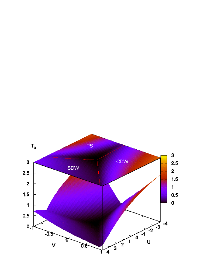
Figure 7: The crossover temperature at $n=1$. The red lines separate $\left(\pi,\pi\right)$ SDW (left), $\left(\pi,\pi\right)$ CDW (right) and PS (on top). Results for negative values of the interaction strength are given for illustrative purposes only. Pairing instabilities may dominate in these cases.

The red lines in Fig. 7 separate three different fluctuation regimes, namely $\left(\pi,\pi\right)$ SDW (on the left), $\left(\pi,\pi\right)$ CDW (on the right) and phase separation (PS) (this is defined by the growth of the zero frequency charge response function at $q_{x}=0$ and $q_{y}=0$). It is noteworthy that the boundary between the SDW and CDW crossover is closely approximated by $U\approx 4V$ (for positive $U$ and $V$), which is in good agreement with previous results Zhang ; Onari ; Oles ; Ohta:1994 ; Yan:1993 ; Bari:1971 . Theory that includes collective modes beyond mean-field also shows deviations from $U=4V$ at weak to intermediate coupling. Yan:1993 Since there are four neighbors which, through $V$, favor charge order while $U$ favors spin order, the crossover at $U\approx 4V$ is expected. In fact, the result $U=zV,$ where $z$ is the number of nearest-neighbors, seems to hold quite generally in various dimensions at $T=0$. Oles ; Fourcade ; Micnas Slightly away from half-filling $\left(n=0.9\right)$ and with a small second-neighbor hopping, the MF approximation Murakami predicts a coexistence region for SDW, CDW and ferromagnetism in the large $U$ and $V$ region of parameter space. This is likely to be an artefact due to an inaccurate estimation of the spin fluctuations in MF when $V\neq 0$. One can see the weakness of this approach by setting $g_{ss}=0$ and ignoring its functional derivative in the equation for the spin susceptibility Eq. (17). These terms are the main source of the suppression of the SDW so that one obviously overestimates the spin effects by ignoring these terms when $V$ is large. One can easily notice that the charge and spin fluctuations appear at relatively large temperature over most of parameter space. In addition, negative $U$ greatly increases charge fluctuations. These will compete with pairing fluctuations that we have not taken into account here. At positive $U$ and $V,$ $d-$wave superconductivity is not likely to occur in regions other than that which is nearly black in the figure.

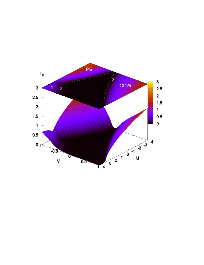
Figure 8: The crossover temperature for $n=0.75$. Results for negative values of the interaction strength are given for illustrative purposes only. Pairing instabilities may dominate in these cases. In the region outside the red line, commensurate (1) SDW $\left(\pi,\pi\right)$, CDW $\left(\pi,\pi\right)$ and PS $\left(0,0\right)$ fluctuations dominate. (The regions of interest are similar to those observed in Fig 7 at $n=1,$ except that SDW become much less important). In the area surrounded by the red and green lines, the renormalized classical fluctuations are incommensurate ISDW in (2) and ICDW in (3). The area inside the green line boundary is paramagnetic. The blue line separates the regions where the spin (left and bottom) and charge (right and top) components of the response functions are dominant.

Fig. 8 shows the crossover diagram for $n=0.75$. The fluctuations outside the red lines are commensurate. The commensurate CDW persists away from half-filling Ohta:1994 while the SDW fluctuations are greatly reduced in the $U>0,V>0$ regime. The fluctuations are incommensurate in the narrow area between the green and red lines. For $U$ and $V$ inside the green curve, the system is paramagnetic, which means that neither the spin nor charge response functions can satisfy the above mentioned criteria even at very low temperature ($T=0.01$). Finally the blue lines separate the region of parameter space where the spin fluctuations are larger than charge fluctuations (left bottom) from the region where the reverse is true (right top). Commensurate fluctuations have the highest crossover temperature. The next most important fluctuations are incommensurate. They exist next to commensurate fluctuations but their crossover temperatures are rather small.

IV Conclusion and Summary

In this paper, we extended the non-perturbative TPSC approach to the case where we add to the standard Hubbard model a nearest-neighbor interaction $V.$ We verified the validity of this Extended Two-Particle Self-Consistent approach (ETPSC) by comparisons with Quantum Monte Carlo calculations. ETPSC applies up to intermediate coupling and it satisfies conservation laws and the Mermin-Wagner theorem. It also includes renormalization of the irreducible vertices by quantum fluctuations (Kanamori-Brückner).

In the original TPSC, the evaluation of the irreducible vertices requires one pair-correlation function and its functional derivative. These two quantities are evaluated by imposing the Pauli principle on two sum rules that lead to self-consistency conditions. In the presence of $V,$ a similar procedure for the irreducible vertices allows us to determine the needed pair correlation functions self-consistently Bahman , but not the functional derivatives of these pair correlation functions. One approach is to neglect the functional derivatives, in the spirit of the Singwi approach Singwi to the electron gas, as we did earlier Bahman . The new idea of the present paper is to use particle-hole symmetry to evaluate the missing functional derivatives. When $V$ is finite, we found that using the resulting estimate of the functional derivatives and dropping one of the sum rules between spin and charge fluctuations implied by the Pauli principle gives better agreement with benchmark QMC than that obtained by neglecting the functional derivatives Bahman . Although particle-hole symmetry strictly applies only to the nearest-neighbor hopping model at half-filling, one expects that the approximation will not be too bad away from half-filling. The results for $n=0.8$ on the bottom right panel of Fig.2 are encouraging in this respect.

For illustrative purposes, we also presented the crossover diagram of the two-dimensional extended Hubbard model on the square lattice for $n=1$ and $n=0.75$ and a range of values of $V$ and $U.$ Incommensurate fluctuations appear away from half-filling, but usually they do so at temperatures much lower than commensurate fluctuations. We highlighted the differences with mean-field calculations Murakami . The crossover temperature indicates when the fluctuations associated with a self-consistently determined wave vector become large, or more specifically when these fluctuations enter the renormalized classical regime. Based on earlier arguments Vilk2 , we expect that a pseudogap appears in the renormalized classical regime whenever the wave vector of the fluctuations can scatter electrons from one side to the other side of the Fermi surface.

The methodology developed in the present paper can be easily applied to different lattices and higher dimension. It can be extended also to longer-range interactions. Note also that the functional derivatives introduce just two independent unknowns, namely $\frac{\delta g_{\uparrow\downarrow}(1,1)}{\delta n(1)}$ and $\frac{\delta g_{s\sigma}(1,2)}{\delta n(1)}=\frac{\delta g_{s\sigma}(1,2)}{\delta m(1)}.$ If there were independent ways of estimating the compressibility and the uniform spin susceptibility, that may give, with the Pauli principle, new sum-rules that could be used to estimate these functional derivatives. That question and that of multiband models are for future research. We also plan to apply ETPSC to specific compounds, such as the cobaltates, where charge fluctuations are important.

V Acknowledgments

We thank S. Hassan and B. Kyung for useful discussions. Computations were performed on the Elix2 Beowulf cluster in Sherbrooke. The present work was supported by the Natural Sciences and Engineering Research Council NSERC (Canada), the Fonds québécois de recherche sur la nature et la technologie FQRNT (Québec), the Canadian Foundation for Innovation CFI (Canada), the Canadian Institute for Advanced Research CIAR, and the Tier I Canada Research Chair Program (A.-M.S.T.).

References

- (1) K. Rosciśzewski and A. Olés, J. Phys. Condens. Matter 15, 8363 (2003).
- (2) Kota Hanasaki, and Masatoshi Imada, J. Phys. Soc. Jpn. 74, 2769 (2005).
- (3) N.E.Bickers, and D.J. Scalapino, Ann. Phys. (USA), 193, 206 (1989).
- (4) Y. M. Vilk, and A. -M. Tremblay, J. Phys. I 7, 1309 (1997).
- (5) Y. M. Vilk, Liang Chen and A.-M. Tremblay, Phys. Rev. B 49, 13267 (1994).
- (6) G.D. Mahan, Many-Particle Physics, 3rd edition, Section 6.4.4 (Kluwer/Plenum, 2000)
- (7) V. Hankevych, B. Kyung, and A.-M. S. Tremblay, Phys. Rev. B 68, 214405 (2003).
- (8) S. Moukouri, S. Allen, F. Lemay, B. Kyung, D. Poulin, Y. M. Vilk, and A.-M. S. Tremblay, Phys. Rev. B 61, 7887 (2000).
- (9) B. Kyung, S. Allen, A.-M. S. Tremblay, Phys. Rev. B 64, 075116 (2001).
- (10) Y. Zhang and J. Callaway, Phys. Rev. B 39, 9397 (1989).
- (11) B. Davoudi and A.M. Tremblay, Phys. Rev. B 74, 035113 (2006).
- (12) R. Pietig, R. Bulla, and S. Blawid, Phys. Rev. Lett. 82, 4046 (1999).
- (13) M. Calandra, J. Merino, and R. H. Mckenzie, Phys. Rev. B. 66 195102 (2002).
- (14) M. Vojta, R.E. Hetzel, R.M. Noack, Phys. Rev. B 60, R8417 (1999).
- (15) M. Vojta, A. Hubsch, R.M. Noack, Phys. Rev. B 63, 045105 (2001).
- (16) H. Seo and H. Fukuyama, J. Phys. Soc. Japan, 67, 2602 (1998).
- (17) A. Hoang, P. Thalmeier, J. Phys.: Condens. Matter 14, 6639 (2002).
- (18) C.S. Hellberg, J. Appl. Phys. 89, 6627 (2001).
- (19) B. Fourcade and G. Sproken, Phys. Rev. B 29, 5096 (1984); J. E. Hirsch, Phys Rev Lett. 53, 2327 (1984); H. Q. Lin and J. E. Hirsch, Phys. Rev. B 33, 8155, (1986).
- (20) L. M. del Bosch and L. M. Falicov, Phys. Rev. B 37, 6037 (1988).
- (21) M. Aichhorn, H.G. Evertz, W. von der Linden, and M. Potthoff, Phys. Rev. B 70, 235107 (2004).
- (22) B M. Bartkowiak, J. A. Henderson, J. Oitmaa, P. E. de Brito, Phys. Rev. B 51, 14077 (1995).
- (23) P. G. J. van Dongen, Phys. Rev. B 49, 7904 (1994); P. G. J. van Dongen, Phys. Rev. B 50, 14016 (1994).
- (24) A. Avella, F. Mancini, Euro. Phys. J. B 41, 149 (2004).
- (25) A. Avella and F. Mancini, J. Phys. Chem. Sol. 67, 142 (2006).
- (26) M. Vojta, Phys. Rev. B 66, 104505 (2002).
- (27) K. Kuroki, J. Phys. Soc. Japan 75, 114716 (2006).
- (28) H. Seo, K. Tsutsui, M. Ogata, and J. Merino, J. Phys. Soc. Japan 75, 117707 (2006).
- (29) S. Onari, R. Arita, K. Kuroki, and H. Aoki, Phys. Rev. B 70, 094523 (2004).
- (30) J. Kishine, H. Namaizawa, Prog. Theor. Phys. 93, 519 (1995).
- (31) J. Callaway, D.P. Chen, D.G. Kanhere, and Qiming Li, Phys. Rev. B 42, 465 (1990) and Physica B 163, 127 (1990).
- (32) D. J. Scalapino, E. Loh, Rr. and J. E. Hirsch, Phys. Rev. B 35, 6694 (1987).
- (33) G. Esirgen and N. E. Bickers, Phys. rev. B 55, 2122 (1997); ibid 57, 5376 (1997)
- (34) X.Z. Yan, Phys. Rev. B 73, 052501 (2006).
- (35) M. Murakami, Journal of the Physical Society of Japan 69, 1113 (2000).
- (36) Y. Ohta, K. Tsutsui, W. Koshibae, and and S. Maekawa, Phys. Rev. B 50, 13594 (1994).
- (37) X.Z. Yan Phys. Rev. B 48, 7140 (1993).
- (38) R.A. Bari, Phys. Rev. B 3, 2662 (1971).
- (39) A.M. Olés, R. Micnas, S. Robaszkiewicz, K.A. Chao, Phys. Lett. A, 102, 323 (1984).
- (40) S. Allen, A.-M. Tremblay and Y. M. Vilk, in Theoretical Methods for Strongly Correlated Electrons, edited by D. Sénéchal, C. Bourbonnais and A.-M. Tremblay, CRM Series in Mathematical Physics, Springer (2003);
- (41) L. P. Kadanoff and G. Baym, Quantum Statistical Mechanics (Benjamin, Menlo Park, 1962).
- (42) K. S. Singwi, M. P. Tosi, R. H. Land and A. Sjölander, Phy. Rev. 176, 589 (1968).
- (43) N.E. Bickers and S.R. White, Phys. Rev. B 43 8044 (1991).
- (44) S. Allen, et A.-M. S. Tremblay, Phys. Rev. B 64, 075115 (2001).