The short-range three-body phase and other issues impacting the observation of Efimov physics in ultracold quantum gases

Abstract

We discuss several issues important for experimentally observing Efimov physics in ultracold quantum gases. By numerically solving the three-boson Schrödinger equation over a broad range of scattering lengths and energies, and by including model potentials with multiple bound states, we address the complications of relating experimental observations to available analytic expressions. These more realistic potentials introduce features that can mask the predicted Efimov physics at small scattering lengths. They also allow us to verify that positive and negative scattering lengths are universally connected only across a pole, not across a zero. Additionally, we show that the spacing between Efimov features for the relatively small scattering lengths accessible experimentally fail to precisely follow the geometric progression expected for Efimov physics. Finally, we emphasize the importance of the short-range three-body physics in determining the position of Efimov features and show that theoretically reproducing two-body physics is not generally sufficient to predict three-body properties quantitatively.

I Introduction

The importance of three-body collisions in determining the lifetime and stability of ultracold atomic gases has been underscored in recent experiments ExpGeneral . Near a Feshbach resonance, for instance, the two-body $s$-wave scattering length $a$ can be made much larger than the characteristic range $r_{0}$ of the interatomic interactions and, due to the strong dependence of the ultracold three-body collision rates on $a$ ScaLenDep , the loss processes can dominate, burning the sample completely or, in other cases, leading to unexpected stability when such collisions are suppressed LLM . In addition to these practical considerations, fundamental effects associated with Efimov physics also appear in the strongly interacting limit $|a|\gg r_{0}$. In the early 1970’s Vitaly Efimov predicted Efimov , in the context of nuclear physics, the existence of a large number of exotic weakly bound trimers that appear whenever $|a|\gg r_{0}$. Only recently, though, has the first experimental evidence of such Efimov states been obtained in ultracold gases Rudi , representing a landmark step for a new generation of experiments designed to explore the rich world of few-body physics.

In ultracold quantum gases, Efimov physics is revealed through its influence on collisions rather than through observation of the states themselves. In this case, Efimov physics can be observed by measuring the time evolution of the atomic or molecular densities and extracting the collision rates Rudi . Efimov physics appears as a series of minima or maxima in these rates as a function of $a$ with the features separated by the multiplicative factor $e^{\pi/s_{0}}$, where $s_{0}=1.00624$ for identical bosons but can vary greatly for other systems EfimovOb . Many of these features are associated with the creation of a new Efimov state in the system.

In this paper we discuss some of the issues that must be considered when attempting to establish connections between analytical predictions for Efimov physics (see, for instance, the reviews BraatenReview ; BraatenReview2 and Ref. ScaLenDep ) and experimental data. These analytic expressions are derived as expansions about $T$=0 and $|a|/r_{0}=\infty$, typically including only the leading term of the expansion. The limitations of these expressions have been explored both in temperature Limits and in scattering length Limits ; Manifestation . In particular, it has been shown that the $|a|\gg r_{0}$ limit is approached only very slowly for many key properties of three-body systems, leading to complications in applying the analytic expressions to experiment since, unfortunately, experiments cannot easily access this limit. Appropriately corrected analytical formulas, although potentially universal themselves, are not yet known BraatenReview ; BraatenReview2 . Perhaps surprisingly, another class of complications arises from the fact that some experiments — even though they are performed at seemingly “ultracold” temperatures — actually lie outside the range of validity Limits of the zero temperature analytical expressions currently available. Finally, there are still other complications that can arise for realistic interatomic potentials that have not been incorporated into the analytical expressions. These complications include, for instance, the finite range of the potentials, the existence of higher angular momentum two-body states, and the multichannel nature of the two-body interaction.

While progress is being made to find more general analytic expressions JonsellEPL ; BraatenPRA ; Koehler ; Stoof ; Platter ; HammerPRA ; PetrovFeshbach , direct numerical solution of the Schrödinger equation currently remains the most reliable approach for non-zero collision energies, finite range potentials, and finite $a$. We present our numerical results for three-boson recombination, $B$+$B$+$B$$\rightarrow$$B_{2}$$+$$B$, using the adiabatic hyperspherical representation HeRecomb ; Limits for a wide range of collision energies. Our calculations show that if the $|a|\gg r_{0}$ condition for Efimov physics is not fully satisfied, then the spacing between Efimov features can be quite far from the predicted $e^{\pi/s_{0}}$. Moreover, we show that if the two-body model has several bound states, then additional resonant effects can appear, complicating the interpretation of Efimov features. We also demonstrate that if $a$ is changed from $+\infty$ to $-\infty$ by crossing $a=0$, then the relation between Efimov states that occur for $a>0$ and $a<0$ is not universal, unlike the case when $a$ changes instead through $|a|=\infty$ across the resonance BraatenReview2 . To illustrate these points, we present numerical results for recombination using model interactions chosen to match the recent Innsbruck Cs experiment Rudi .

Finally, we discuss the importance of the short-range three-body physics in determining the precise position of the Efimov features. In our work, this physics is parameterized by a short-range phase (also in Ref. MacekRecomb ), whereas effective field theory treatments have various parameterizations generally equivalent to a momentum cutoff Efimov ; BraatenReview . This three-body parameter cannot, however, be determined from knowledge of the near-threshold two-body physics. Consequently, fitting the near-threshold two-body observables Koehler ; Stoof alone is not sufficient to accurately predict the position of the Efimov features, no matter how complete. To make this point clear, we show that including a non-pairwise-additive three-body interaction AxilrodTeller ; Launay , known to be present in every triatomic system, changes the positions of the Efimov features, which is equivalent to changing the short-range three-body phase JPBDAMOPPoster . So, even if the “exact” two-body potentials were used instead of just the near threshold fit, the positions of the Efimov features could not be quantitatively predicted.

II Theoretical Method

Our method for solving the three-body Schrödinger equation has been detailed elsewhere HeRecomb ; Limits , but we include a brief description here for completeness and clarity.

II.1 Adiabatic hyperspherical representation

We solve the three-body Schrödinger equation using the adiabatic hyperspherical representation Macek68 ; HeRecomb . After the usual separation of the center-of-mass motion, the three-body problem can be described by the hyperradius $R$ and five hyperangles, denoted collectively by $\Omega$. The hyperangular part of the Schrödinger equation determines the relative motion of the three bodies, and the hyperradial part determines the overall size of the system. The five angular coordinates are chosen to be the Euler angles ($\alpha$, $\beta$, and $\gamma$), specifying the orientation of the plane defined by the three particles relative to the space-fixed frame, plus two hyperangles ($\theta$ and $\varphi$) defined as a modified version of Smith-Whitten coordinates HeRecomb ; Smith .

The Schrödinger equation in hyperspherical coordinates can be written in terms of the rescaled wave function $\psi=R^{5/2}\Psi$ as (in atomic units)

$$\left[-\frac{1}{2\mu}\frac{\partial^{2}}{\partial R^{2}}+H_{ad}(R,\Omega)\right]\psi(R,\Omega)=E\psi(R,\Omega),$$ (1)

where $\mu$ is the three-body reduced mass ($\mu=m/\sqrt{3}$ for three identical bosons of atomic mass $m$) and $E$ is the total energy. The adiabatic Hamiltonian $H_{ad}$ in Eq. (1) is given by

$$H_{ad}(R,\Omega)=\frac{\Lambda^{2}+15/4}{2\mu R^{2}}+V(R,\theta,\varphi).$$ (2)

In this expression, $\Lambda^{2}$ is the hyperangular kinetic energy; and $V$, the potential energy. The eigenfunctions $\Phi_{\nu}$ of $H_{ad}$,

$$H_{ad}(R,\Omega)\Phi_{\nu}(R;\Omega)=U_{\nu}(R)\Phi_{\nu}(R;\Omega),$$ (3)

form a complete, orthonormal basis at each $R$. Tthe total wave function $\psi(R,\Omega)$ can thus be written as

$$\psi(R,\Omega)=\sum_{\nu}F_{\nu}(R)\Phi_{\nu}(R;\Omega),$$ (4)

where $\nu$ is a collective index that includes all the quantum numbers necessary to identify each channel. If the expansion in Eq. (4) includes the complete, countably-infinite set of $\Phi_{\nu}$, $\psi(R,\Omega)$, then this representation of $\psi$ is in principle exact. In practice, of course, the sum is truncated to a finite number of terms, but it can be extended systematically to obtain essentially any desired level of accuracy. The eigenvalues $U_{\nu}(R)$ of Eq. (3) give the potential curves.

Substituting Eq. (4) into the full Schrödinger equation (1) and projecting out $\Phi_{\nu}$ gives the hyperradial Schrödinger equations — a system of coupled ordinary differential equations:

$$\left(-\frac{1}{2\mu}\frac{d^{2}}{dR^{2}}+U_{\nu}(R)\right)F_{\nu}(R)-\frac{1}{2\mu}\sum_{\nu^{\prime}}\left(2P_{\nu\nu^{\prime}}(R)\frac{d}{dR}+Q_{\nu\nu^{\prime}}(R)\right)F_{\nu^{\prime}}(R)=EF_{\nu}(R).$$ (5)

The nonadiabatic coupling terms $P_{\nu\nu^{\prime}}(R)$ and $Q_{\nu\nu^{\prime}}(R)$ are generated by the hyperradial dependence of the channel functions and are responsible for inelastic transitions. They are defined as

$$P_{\nu\nu^{\prime}}(R)=\left<\!\!\!\left<\!\Phi_{\nu}(R)\left|\frac{d}{dR}\right|\Phi_{\nu^{\prime}}(R)\!\right>\!\!\!\right>$$ (6)

and

$$Q_{\nu\nu^{\prime}}(R)=\left<\!\!\!\left<\!\Phi_{\nu}(R)\left|\frac{d^{2}}{dR^{2}}\right|\Phi_{\nu^{\prime}}(R)\!\right>\!\!\!\right>.$$ (7)

The double brackets indicate integration only over the angular coordinates $\Omega$ and traces over any spin degrees of freedom, with the hyperradius $R$ fixed.

The $S$-matrix elements — and thus cross sections and rates — are found from the solutions of Eq. (5) Aymar . The main focus of this work, the three-body recombination rate $K_{3}$, is obtained from the $S$-matrix as follows OurFirstPRL ; HeRecomb :

$$K_{3}=\sum_{J,\pi}\sum_{i,f}\frac{192(2J+1)\pi^{2}}{\mu k^{4}}|S^{J\pi}_{f\leftarrow i}|^{2},$$ (8)

where $k=\sqrt{2\mu E}$ is the incident hyperradial wave number, $i$ labels the initial continuum channel, and $f$ labels the final two-body channels. This expression also reflects the fact that we use the total orbital angular representation since the total orbital angular momentum $J$ is conserved. Total parity $\pi$ is also a good quantum number labeling the $S$-matrix.

II.2 Two-body potential model

The potential $V$ used in Eq. (2) for the present calculations is a sum of atom-atom interactions, $V=v(r_{12})+v(r_{31})+v(r_{23})$, which is most appropriate for spin-stretched atoms. We take advantage of universality to use a two-body model potential for $v(r_{ij})$ that is computationally convenient. That is, the Efimov effect and other low-energy three-body properties do not depend on the details of the interatomic interaction, only on the scattering length and the characteristic length scale $r_{0}$ of the potential. The primary simplification this allows is to reduce the number of two-body ro-vibrational bound states from hundreds or thousands, for realistic triplet alkali potentials, to something more manageable.

The two-body potential model adopted here is

$$v(r)=D\,{\rm sech}^{2}\left(\frac{r}{r_{0}}\right)$$ (9)

where $D$ is the potential strength. With this potential, we can easily produce two-body systems with different values of the scattering length and different numbers of bound states by changing $D$ OurFirstPRL ; Manifestation .

In Fig. 1 we show the scattering length as a function of $D$. The first pole in $a$ (as $D$ grows increasingly negative, starting from $D=0$) occurs when the first $s$-wave bound state is formed. The second pole in $a$ (as $|D|$ increases) occurs when a second $s$-wave bound state is formed. Our rate calculations cover regions I and II. In addition to having one more $s$-wave bound state than region I, region II also has a $d$-wave two-body state that becomes bound at the value of $D$ indicated in the figure. As we will see below, this $d$-wave state leads to resonance effects in the three-body recombination rate that could be misinterpreted as an Efimov feature.

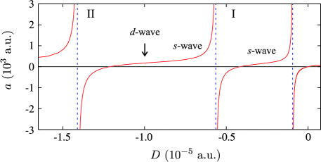
Figure 1: Scattering length as a function of the potential depth for $v(r)$ from Eq. (9). There is one $s$-wave bound state in region I but there are two in region II. A $d$-wave bound state is also created in region II.

III Results and Discussion

The fact that three-body recombination can be the main loss mechanism in ultracold atomic gases is what made Efimov physics observable in the recent experiments of Kraemer et al. Rudi . For $a>0$, the recombination rate at $T$=0 shows a series of minima, resulting from interference between two different pathways OurFirstPRL ; MacekRecomb . The rate can be conveniently written as

$$K_{3} =67.1e^{-2\eta_{M}}\!\!\left[\sin^{2}[s_{0}\ln(\frac{a}{r_{0}})+\Phi_{M}]+\sinh^{2}\eta_{M}\right]\frac{\hbar a^{4}}{m}$$

$$+16.8(1-e^{-4\eta_{M}})\frac{\hbar a^{4}}{m},$$ (10)

including the contributions from both weakly- and deeply-bound molecules OurFirstPRL ; MacekRecomb ; BraatenReview . For $a<0$, though, the mechanism that produces signatures of Efimov physics is quite different and is related to resonant transmission effects that occur when an Efimov state is created OurFirstPRL . For $a<0$, the $T$=0 recombination rate is BraatenReview

$$K_{3}=\frac{4590\sinh(2\eta_{P})}{\sin^{2}[s_{0}\ln(|a|/r_{0})+\Phi_{P}]+\sinh^{2}{\eta_{P}}}\frac{\hbar|a|^{4}}{m}.$$ (11)

In these equations, $\Phi_{M}$ and $\Phi_{P}$ are short-range three-body phases that determine the positions of the minima and peaks, respectively. The parameters $\eta_{M}$ and $\eta_{P}$ were introduced BraatenReview to characterize the probability of an inelastic transition at small distances to a deeply bound molecule. In practice, $\Phi$ and $\eta$ are used as fitting parameters since the short distance behavior of realistic systems is not generally known. We have found Limits that Eqs. (10) and (11) are good approximations at all collision energies $E$ and scattering lengths $a$ in the threshold regime, i.e. $E\lesssim\hbar^{2}/2\mu_{\rm 2b}a^{2}$ where $\mu_{\rm 2b}$ is the two-body reduced mass.

III.1 Fitting experiment

In Fig. 2(a) we show our numerical results for the thermally averaged HeRecomb ; Limits recombination length $\varrho_{3}$ of ¹³³Cs atoms, along with the experimental data obtained in the Innsbruck experiment Rudi . Our data were generated for the same range of scattering lengths (in region I of Fig. 1) and temperatures accessed experimentally, including the two leading-order contributions, $J^{\pi}=0^{+}$ and $2^{+}$, to Eq. (8) Limits . Even though we used a simple two-body model potential, our results for $a<0$ and $a>0$ reproduce the experimental data quite well. In our approach, the only adjustable parameter is $r_{0}$. We obtained $r_{0}$$\approx$100 a.u. by fitting the experimental peak position, $a\approx-850$ a.u., at $T$=10 nK. We used this same $r_{0}$ to produce the curves for the other temperatures and for $a>0$. We will discuss the validity of the latter in Sec. III.3.

It is important to note that although our numerical value for $r_{0}$ happens to agree with the expected result for Cs atoms — namely, the van der Waal’s length $r_{vDW}$ Julienne — it unfortunately does not imply that we can predict the peak position for this or any other species. The reason is that our choice of model two-body potential Eq. (9) determines the short-range physics and has no particular relation to the correct short-range physics for three Cs atoms. A different choice of model potential would lead to a different best fit value for $r_{0}$. The model potential thus sets the values of $\Phi$ and $\eta$, preventing their use as fit parameters. In fact, any finite range two-body model potential Koehler ; Stoof will suffer from essentially the same problem, as we will discuss in more detail in Sec. III.4.

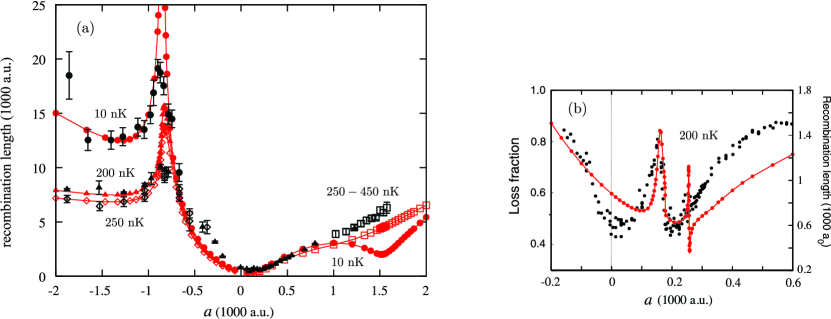
Figure 2: (Color online) (a) Comparison between ¹³³Cs recombination length, $\varrho_{3}=(mK_{3}/\hbar\sqrt{3})^{1/4}$ OurFirstPRL , obtained experimentally Rudi (black symbols) and our present thermally averaged results (red symbols). Filled circles and triangles were obtained at 10 and 200 nK, respectively; open diamonds and squares were obtained at 250 nK and 250–450 nK, experimentally, and at 250 nK in the present calculation. (b) Effect of the $d$-wave resonance on the thermally averaged recombination length for small values of $a$ in region II of Fig. 1 in comparison to the observed loss fraction from Rudi .

The major difference between our results in Fig. 2(a) and the experimental results lies at $a>0$. As it turns out, we would not expect good agreement since our $a>0$ results use the same $r_{0}$ as the $a<0$ results. As already noted, this point will be discussed in detail in Sec. III.3, but the $a>0$ results in Fig. 2(a) do serve to illustrate the important role of temperature for attempts to observe the minimum. Figure 2(a) shows, for instance, that at $10$ nK we do find a minimum at $a=1500$ a.u.. At 250 nK, however, strong contributions from the next partial wave, $J^{\pi}=2^{+}$ Limits , mask the minimum. Comparison with the experimental data shows that even if there were actually a minimum for Cs that matched our model, the experimental temperature was likely just too high to be able to see it. For heavy atoms like Cs, the requirement of being in the threshold regime to see Efimov features Limits places a relatively severe limit on the maximum allowable temperature.

III.2 Finite range potentials

Analytic expressions for $K_{3}$ such as Eqs. (10) and (11) were derived as an expansion about $|a|\gg r_{0}$. In practice, this was accomplished using zero-range two-body interactions that support at most one $s$-wave bound state. Calculations performed using a finite range potential like Eq. (9) produce deviations from these analytical predictions and introduces features not observable with these zero-range potentials. One immediate consequence of a non-zero $r_{0}$ is that the minimum observed in the Cs experiment around $a=210$ a.u. is likely not related to Efimov physics since $a$ is not much larger than $r_{0}=r_{vDW}\approx$100 a.u. This point was, in fact, already noted in Ref. Rudi . We have found Manifestation that for most quantities the predictions of the zero-range model are recovered in a reasonably quantitative way only when $|a|$ is more than an order of magnitude larger than $r_{0}$.

In this range of scattering lengths, the recombination rate for finite range potentials can have structure that is completely independent of Efimov physics JPBDAMOPPoster . This structure is generated by the presence of non-$s$-wave two-body states. Figure 2(b) shows an example of such structure due to a $d$-wave two-body state. It shows our numerical results for $\varrho_{3}$, now obtained for $a$ in region II (with two $s$-wave bound states). These results display behavior similar to the experimental observations, represented in this figure by the loss fraction reported in Ref. Rudi . A minimum (or peak) in the recombination rate does lead to a minimum (or peak) in the loss fraction, and vice-versa, so the figures can be compared qualitatively. As the scattering length is decreased from its maximum in the figure, the two-body $d$-wave state can be visualized as approaching the threshold from above. While above the threshold, the $d$-wave state is a two-body shape resonance; below threshold, it is, of course, a bound state. Thus, the first, sharp feature as $a$ is decreased, at $a\approx 280$ a.u., is produced when the two-body shape resonance energy matches the three-body collision energy NJP . Physically, this situation can be thought of as ro-vibrational relaxation of the two-body resonant state. Two atoms collide, forming a $d$-wave two-body resonance, when the third atom collides with it, driving it down into the available $s$-wave bound states. It is interesting to note that the total orbital angular momentum is $J=0$, whereby the relative angular momentum of the initial atom-dimer complex must also be a $d$-wave. The final angular momentum of the bound dimer is zero as must be the relative atom-dimer angular momentum. There is thus considerable angular momentum and energy exchange at work near this feature. The next broad feature at smaller $a$ occurs where this two-body resonance becomes a bound state. Being the highest-lying bound state, it receives the majority of the recombination.

It is worth noting that this $d$-wave $K_{3}$ resonance does not correspond to a resonance in $a$ because it is an open channel two-body shape resonance — not a resonance in the $s$-wave channel. Higher partial wave resonances in $a$ are typically due to higher order two-body interactions coupling the incident $s$-wave to a closed channel resonances Chin . The appearance of higher partial wave resonances at moderate scattering lengths is a generic feature that has been examined in detail for van der Waals interactions in Ref. Gao . The two-body interaction for most any atoms will generally support not only $d$-wave bound states and resonances, but also much higher angular momentum states, potentially leading to considerably more structure near $a=0$.

We emphasize that the comparison in Fig. 2(b) is only an illustration of the complications that can occur in realistic systems, especially in the non-universal region of $|a|\approx r_{0}$. A definitive interpretation of the $a>0$ experimental data requires incorporating considerably more information about the Cs-Cs interaction into our model than we have. Fortunately, much is known about the Cs-Cs interaction, and the scattering length has been calculated as a function of magnetic field with some confidence Chin . With that information, and the additional universal relations between $s$-wave and $d$-wave states for alkali atoms Gao , it should be possible to locate any higher partial wave open-channel resonances to check whether features like the $d$-wave $K_{3}$ resonance in Fig. 2(b) are possible.

Further complicating any effort to identify Efimov features in this range of $a$, the global minimum in $K_{3}$ lies at $a\approx 200$ a.u. — even without the $d$-wave resonance. The global minimum can be see in both Figs. 2(b) and (c), showing that recombination goes through a minimum when $a$ is tuned from $a\rightarrow\infty$ and $a\rightarrow-\infty$ through $a=0$.

To further illustrate the effect of finite range two-body potentials, we show in Fig. 3 the recombination rate obtained for fixed collision energies from $0.67\times 10^{-4}$ nK up to $670$ nK and $|a|$ up to $2\times 10^{6}$ a.u. across regions I and II of Fig. 1. These rates include only the $0^{+}$ contribution and are not thermally averaged, so the indicated “temperatures” are the collision energies converted to Kelvin. The rates in Figs. 3(a) and 3(b) were obtained for $a$ in region II and therefore have up to three contributions: recombination into the two possible $s$-wave states and into the $d$-wave state. The rates in Figs. 3(c) and 3(d) were obtained for $a$ in region I and represent recombination into the single available $s$-wave bound state. Figures 3(a) and (b) thus connect across a zero in the scattering length; (b) and (c), across a pole; and (c) and (d), across a zero. Comparing the partial rates in Figs. 3(b) and (c) for energies from 6.7$\times 10^{-2}$ nK up to 670 nK, recombination into the lowest $s$-wave bound state is smooth across the resonance where the second $s$-wave bound state is formed. For lower energies this connection should also be smooth, but will happen only for larger values of $a$. Recombination into the second $s$-wave bound state in Fig. 3(b) introduces a discontinuity in the total recombination rate at non-zero collision energies. It would apprear from Fig. 3(b) that the appearance of the $d$-wave bound state near $a$=0 also introduces a discontinuity, but because the relative angular momentum between the atom and dimer in the final state is $d$-wave, the Wigner threshold law guarantees that it will turn on smoothly.

Figure 3(a) shows that recombination into the $d$-wave state actually dominates over the whole range of $a$ in this panel, which is not too surprising since it is the most weakly bound dimer state. Moreover, the $d$-wave partial rate shows the expected Efimov features — as do all of the partial rates in Fig. 3(a) — emphasizing that the Efimov physics is determined for $a<0$ by the initial three-body state and not the final state ScaLenDep ; OurFirstPRL ; MacekRecomb . This dependence is one way to understand the universality of $K_{3}$ for $a<0$ since the initial channel is universal while the final, deeply bound states are not.

One other issue evident from comparing the analytical curves in Fig. 3 to the calculated ones is that the expected spacing between Efimov features does not hold between the two features nearest $a$=0. In Figs. 3(c) and 3(d), the spacing between the first two minima and first two peaks are 28.3 and 14.3, respectively, instead of the 22.7 expected for identical bosons. The spacing between the next two minima and peaks are 23.4 and 21.6, respectively. Where the spacing can be defined in Figs. 3(a) and (b), it follows the same pattern. This sort of deviation for the spacing of the first few features is important to be recognized by any experiment seeking to verify the logarithmic spacing of Efimov features. At least in the near future, experiments will likely not be able to observe more than a few of these features nearest to $a=0$, in view of the large range in $a$ and the low temperatures required EfimovOb . So, knowing the finite range corrections to the logarithmic spacing, and knowing whether those corrections are universal, are both critical.

III.3 Tuning $a$ from $-\infty$ to $+\infty$

In addition to the complications discussed above, fundamental issues were raised in Ref. Rudi since the scattering length was tuned from $-\infty$ to $+\infty$ through $a=0$ and therefore through a non-universal region. In fact, $a$ was tuned through a series of narrow resonances. While this was obviously the expedient choice experimentally, it is not obvious that the $a<0$ and $a>0$ Efimov features should retain their universal relation predicted from the zero-range model BraatenReview ,

$$\Delta\Phi=\Phi_{M}-\Phi_{P}=-1.53(3),$$ (12)

or even that the short-range three-body phase on each side of a narrow resonance should be universally related, let alone the same. Clearly, it is convenient if these relations hold since only one phase is then required to predict the position of both minima ($a>0$) and peaks ($a<0$). So, the question that naturally arises is whether there is a relation similar to Eq. (12) between the peak and minimum positions when $a$ is tuned across a non-universal region ($a=0$). To explore this issue, we analyze the relations between the numerical calculations shown in the panels of Fig. 3. The fact that $K_{3}$ for $a<0$ and $a>0$ are universally related only across a pole in $a$, and the resulting consequences for the Cs experiment, have been raised in previous work BraatenReview2 ; Koehler . Here, however, we show via a counter-example that there is no general universal connection across a zero in $a$.

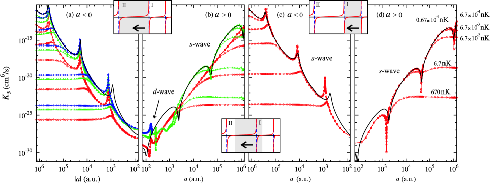
Figure 3: (Color online) Recombination rate for $a$ covering regimes with different numbers of two-body bound states, as indicated above. In (a) and (b) recombination has contributions from the deeply (red circles) and weakly (green triangles) bound $s$-wave states as well as from the $d$-wave state (blue diamonds). The lines without symbols are the fit of Eqs. (10) and (11).

Because of the slow approach of the system’s properties to the $|a|\gg r_{0}$ predictions and the requirement of being in the threshold regime, the range of scattering lengths and temperatures required to observe more than one feature in ¹³³Cs, necessary to determine $\Phi$ precisely from Eqs. (10) and (11), greatly exceeds current experimental capabilities. This fact underscores the advantages of using different atomic species to make the required range of $a$ and $T$ much more reasonable EfimovOb .

The three-body phases $\Phi_{P}$ and $\Phi_{M}$ were determined from our numerical results in Fig. 3 by independently fitting Eqs. (10) and (11) to the positions of the peaks and minima at our largest $|a|$ and lowest temperature in order to better satisfy the approximations under which those equations were derived. The fit curves are indicated in Fig. 3 by the line without symbols. From Figs. 3(b) and 3(c), which should be connected universally since they cross a pole in $a$, we obtain $\Delta\Phi_{bc}$=$-$1.553, in good agreement with Eq. (12). The other phase differences — which imply crossing a non-universal region — are, however, $\Delta\Phi_{ab}$=$-$1.053 and $\Delta\Phi_{cd}$=$-$1.381. Thus, the Efimov physics for $a$$>$0 and $a$$<$0 do not appear to be simply connected when separated by a non-universal region.

We rationalize this non-universal behavior by recognizing that small changes in the interactions should not substantially affect the short range physics, i.e. $\Phi$ and $\eta$. Changing $a$ from positive to negative across a resonance requires a much smaller change in the interactions than does crossing $a=0$, so the former should lead to universal behavior. The relative changes required in the depth of the potential $D$ when crossing each region are clearly illustrated in Fig. 1. Similarly, when controlling $a$ via a Feshbach resonance, going from $a>0$ to $a<0$ requires smaller changes in the magnetic field when crossing a resonance than when crossing $a=0$. It is not entirely clear, however, whether this argument generalizes directly from our model potentials to realistic potentials with many bound states since the relative change in such a realistic potential when crossing $a$=0 will also be small. In principle, we can answer this question by simply continuing to increase $D$ and solving the problem numerically. Unfortunately, we are not yet able to calculate the three-body recombination in a system with more than a handful of two-body bound states. Incidentally, we expect similar behavior for the other short-range three-body parameter $\eta$. Specifically, we expect $\eta_{P}=\eta_{M}$ when $a$ is tuned across a resonance, but not when it is tuned across $a=0$.

In the Innsbruck experiment, $\Delta\Phi$ was found in the form of the ratio

$$\frac{a_{+}}{|a_{-}|}=\exp[{-(\Delta\Phi+\pi/2)/s_{0}}].$$ (13)

Experimentally, $a_{+}$ located the first recombination maximum near $a=0$ for $a>0$; and $a_{-}$, the first peak for $a<0$. The experimental fit gave $a_{+}/|a_{-}|\approx 1.25(9)$ Rudi . Considering that the phases in $\Delta\Phi$ are defined as mod $\pi$, with $\Phi_{M}$ and $\Phi_{P}$ defined in the range $[0,\pi)$, the minimum and maximum values for $a_{+}/a_{-}$ are respectively 0.00925 and 4.76385, this result agrees relatively well with the theoretical value of 0.96(3). Theoretically, however, $\Delta\Phi$ is defined from the $|a|\gg r_{0}$ limit. Our $\Delta\Phi_{bc}$, for instance, was determined by fitting in this limit and gives $a_{+}/|a_{-}|$=0.982. The proper comparison with experiment, using the first features in Figs. 3(b) and 3(c), is difficult to make, though, since there is no clear maximum for small positive $a$ — save for the $d$-wave resonance — to define $a_{+}$. If there were, it would likely be smaller than predicted by Eq. (10) (compare with the solid line fit). On the other hand, $a_{-}$ would be larger than predicted, giving $a_{+}/|a_{-}|$ smaller than the $|a|\gg r_{0}$ prediction — assuming these feature shifts are universal. We can also get a sense of the quality of the agreement between theory and experiment by calculating $a_{+}/|a_{-}|$ from $\Delta\Phi$ across a non-universal region: $\Delta\Phi_{cd}$, for instance, gives $a_{+}/|a_{-}|$=0.828; $\Delta\Phi_{ab}$ gives 0.598. Both of these values are nearly as close to the predicted value as the experiment, but we know that the present “agreement” is accidental. So, the fact that the experiment accessed the non-universal region together with the fact that the minimum position ($a=210$ a.u.) is not firmly in the universal regime ($a\gg r_{0}$), make us believe that the agreement between experiment and theory for $a_{+}/|a_{-}|$ is likely fortuitous.

III.4 Three-body short-range physics

It should be clear by now that knowledge of the short-range three-body phase is essential to make quantitative theoretical predictions for ultracold three-body recombination of realistic systems — or, indeed, for nearly any ultracold three-body process. The three-body phase can be determined from essentially any ultracold three-body observable, and many examples have been discussed in Ref. BraatenReview . It should be equally clear from the discussion of Fig. 3 that fitting a two-body model potential to give the correct scattering length is not sufficient to determine the three-body phase. Even a more complete fitting of the low-energy two-body physics Koehler ; Stoof will not give the correct three-body phase. In fact, quantitative predictions for real systems would not be possible even if the complete two-body interaction were included in the calculation. The reason is simple: in real triatomic systems, there is a short-range, non-additive, purely three- body interaction AxilrodTeller ; Launay . So, model calculations such as ours and those in Refs. Koehler ; Stoof ,

that fit only two-body physics fundamentally cannot predict the positions of Efimov features quantitatively without the input of a known near-threshold three-body observable — because of the three-body short-range physics.

To illustrate the effects of non-additive three-body interactions, we have performed calculations that include one such correction. We have included the well-known three-body Axilrod-Teller potential AxilrodTeller which, analogous to the two-body van der Waals interaction, is the leading-order dispersion term describing the long- range induced dipole-dipole-dipole interaction among three neutral atoms. The Axilrod-Teller potential assumes the following form,

$$W_{AT}(r_{12},r_{23},r_{13})=\gamma\frac{(1+3\cos\theta_{12}\cos\theta_{23}\cos\theta_{31})}{r_{12}^{3}r_{23}^{3}r_{31}^{3}},$$ (14)

where $r_{ij}$ are the interatomic distances and $\theta_{ij}=\cos^{-1}(\hat{r}_{ik}\cdot\hat{r}_{jk})$ are the inner angles of the triangle formed by the three atoms. In the above equation $\gamma$ is a positive quantity whose exact value depends on the details of the three-body system. Note that this interaction can be attractive or repulsive depending upon the shape of the three atom system. It is also worth emphasizing that the Axilrod-Teller interaction is just one of several short-range three-body interactions that can affect three-body observables. In fact, much stronger corrections are expected due to purely three-atom exchange effects Launay .

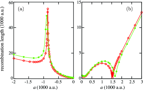
Figure 4: (color online) Comparison of the (a) peak and (b) minimum position in the recombination length with the Axilrod-Teller interaction (green filled circles) and without it (red open circles). These calculations demonstrate that the main effect of the inclusion of the Axilrod-Teller potential is to move the position of the minimum and peak as shown above.

While $\gamma$ in Eq. (14) normally reflects the details of the atoms, for the purposes of our model, we have chosen it to have the form

$$\gamma=\gamma_{0}|D|r_{0}^{9}[\tanh(\frac{r_{12}}{r_{0}})\tanh(\frac{r_{23}}{r_{0}})\tanh(\frac{r_{31}}{r_{0}})]^{3}.$$ (15)

This choice ensures that $W_{AT}$ scales as we tune the two-body scattering length, that it scales properly with $r_{0}$, and that the $r_{ij}^{-3}$ singularities are cut off near $r_{ij}=0$. We have arbitrarily chosen a value for $\gamma_{0}$ that causes a variation of about 15% in the adiabatic hyperspherical potentials near the minimum. This magnitude change is probably an underestimate, given that it has been shown that non-additive three-body terms make the minimum in the three-atom potential surface from 60% to a factor of four deeper for alkali atom systems, compared to the pairwise additive potential surface Hutson ; HutsonLaunay ; HutsonPRA .

Figure 4 shows the recombination length with and without the Axilrod-Teller term. Our results in the figure demonstrate that the minimum and peak positions are clearly shifted by the inclusion of the Axilrod-Teller term. For $a<0$, besides changing the peak position, the Axilrod-Teller interaction also changes the width of the resonance peak and the overall amplitude of recombination length. This result indicates that the coupling to deeply bound decay channels is also affected by the Axilrod-Teller interaction. The analytic expressions in Eqs. (10) and (11) account for these effects through changes to the short-range parameters $\Phi$ and $\eta$.

Our results in Fig. 4, therefore, demonstrate our initial statement. The inclusion of purely three-body interactions such as the Axilrod-Teller — or the three atom exchange — are of crucial importance for accurately predicting features related to Efimov physics. As a consequence, even though previous works have rather carefully fit the two-body physics Koehler ; Stoof , it is unlikely that they have predictive power in locating Efimov features.

IV Summary

Using essentially exact numerical solutions for a model two-body potential, we have demonstrated the need for caution when applying existing analytic expressions for three-boson recombination to experiment. While they do give considerable insight, their predictions for the first features near $a$=0 are not quantitative and may even fail qualitatively due to the complications arising from realistic potentials — in particular, from their finite range. Moreover, care must be taken to ensure that the temperature is truly in the threshold regime. We have also verified quantitatively that $a>0$ features are universally connected to $a<0$ features only when $a$ is tuned through $|a|=\infty$ of a given resonance.

Finally, we have emphasized the importance of the short-range three-body phase in making quantitative predictions for real systems. This point does not appear to be fully appreciated theoretically, but our example of the non-additive three-body term underscores the limitations of purely two-body models for actual triatomic systems and thus the need for a three-body parameter. Unfortunately, purely ab initio calculation of this three-body parameter seems, for now, out of reach for the systems of experimental interest.

- (1) C. A. Stan, M. W. Zwierlein, C. H. Schunck, S. M. F. Raupach, and W. Ketterle, Phys. Rev. Lett. 93, 143001 (2004); S. Inouye et al., ibid. 93, 183201 (2004); T. Weber et al., ibid. 91, 123201 (2003).
- (2) J. P. D’Incao and B. D. Esry, Phys. Rev. Lett. 94, 213201 (2005); Phys. Rev. A 73, 030702(R) (2006).
- (3) J. Cubizolles et al., Phys. Rev. Lett. 91, 240401 (2003); S. Jochim et al., ibid. 91, 240402 (2003); K. E. Strecker et al., ibid. 91, 080406 (2003); C. A. Regal, M. Greiner, and D. S. Jin, ibid. 92, 083201 (2004).
- (4) V. Efimov, Sov. J. Nucl. Phys. 12, 589 (1971); 29, 546 (1979); Nucl. Phys. A210, 157 (1973).
- (5) T. Kraemer, M. Mark, P. Waldburger, J. G. Danzl, C. Chin, B. Engeser, A. D. Lange, K. Pilch, A. Jaakkola, H.-C. Nägerl and R. Grimm, Nature 440, 315 (2006).
- (6) J. P. D’Incao and B. D. Esry, Phys. Rev. A 73, 030703(R) (2006).
- (7) J. P. D’Incao, H. Suno, and B. D. Esry, Phys. Rev. Lett 93, 123201 (2004).
- (8) J. P. D’Incao and B. D. Esry, Phys. Rev. A 72, 032710 (2005).
- (9) E. Braaten and H. -W. Hammer, Phys. Rep. 428, 259.
- (10) E. Braaten, H.-W. Hammer, Ann. Phys. 322, 120 (2007).
- (11) B. D. Esry, C.H. Greene, and J. P. Burke, Phys. Rev. Lett. 83, 1751 (1999). Note that the coefficient in the rate equation for in this paper was too large by a factor of six; the coefficient in Eq. (8) is the correct one.
- (12) E. Nielsen and J. H. Macek, Phys. Rev. Lett. 83, 1566 (1999).
- (13) T. Köhler, K. Góral, and P. S. Julienne, Rev. Mod. Phys. 78, 1311 (2006).
- (14) H. Suno, B. D. Esry, and C. H. Greene, New J. Phys. 5, 53 (2003).
- (15) C. Chin, et al., Phys. Rev. A 70, 032701 (2004).
- (16) Bo Gao, J. Phys. B 37, 4273 (2004); Phys. Rev. A 62, 050702(R) (2000).
- (17) J.P. Burke, B.D. Esry, C.H. Greene, DAMOP 2000, Bull. Am. Phys. Soc. 45, 67 (2000).
- (18) S. Jonsell, Europhys. Lett. 76, 8 (2006)
- (19) E. Braaten, D. Kang, and L. Platter, Phys. Rev. A 75, 052714 (2007).
- (20) M. D. Lee, T. Koehler, P. S. Julienne, Phys. Rev. A 76, 012720 (2007); G. Smirne, R. M. Godun, D. Cassettari, V. Boyer, C. J. Foot, T. Volz, N. Syassen, S. Dürr, G. Rempe, M. D. Lee, K. Góral,1 and T. Köhler, Phys. Rev. A 75, 020702(R) (2007).
- (21) P. Massignan and H. T. C. Stoof, arXiv:cond-mat/0702462.
- (22) B. M. Axilrod and E. Teller, J. Chem. Phys. 11, 299 (1943).
- (23) M. T. Cvita, P. Soldán, J. M. Hutson, P. Honvault, and J.-M. Launay, J. Chem. Phys. 127, 074302 (2007); E. E. Polymeropoulos, J. Brickmann, L. Jansen, and R. Block, Phys. Rev. A 30, 1593 (1984).
- (24) H. Suno, B.D. Esry, C.H. Greene, and J.P. Burke, Jr., Phys. Rev. A, 65, 042725 (2002).
- (25) R.C. Whitten and F.T. Smith, J. Math. Phys. 9, 1103 (1968).
- (26) J. Macek, J. Phys. B 1, 831 (1968).
- (27) M. Aymar, C.H. Greene, and E. Luc-Koenig, Rev. Mod. Phys. 68, 1015 (1996).
- (28) L. Platter and D.R. Phillips, Few-Body Systems 40, 35 (2006).
- (29) H.W. Hammer, T.A. Lähde, and L. Platter, Phys. Rev. A 75, 032715 (2007).
- (30) D. Petrov, Phys. Rev. Lett. 93, 143201 (2004).
- (31) M.T. Cvitaš, P. Soldán, and J.M. Hutson, Mol. Phys. 104, 23 (2006).
- (32) P. Soldán, M.T. Cvitaš, J.M. Hutson, P. Honvault, and J.M. Launay, Phys. Rev. Lett. 89, 153201 (2002).
- (33) P. Soldán, M.T. Cvitaš, and J.M. Hutson, Phys. Rev. A 67, 054702 (2003).