Phase Transition in a Two-level-cavity System in an Ohmic Environment

Abstract

We propose that in the presence of an Ohmic, de-phasing type environment, a two-level-cavity system undergoes a quantum phase transition from a state with damped Rabi oscillation to a state without. We present the phase diagram and make predictions for pump and probe experiment. Such a strong coupling effect of the environment is beyond the reach of conventional perturbative treatment.

A combined two-level system and an cavity electromagnetic mode has been proposed as an important realization of qubit in quantum information scienceraimond ; mabuchi ; stievater ; wall . In quantum optics the coherent oscillation, or Rabi oscillation, of such a combined system is the key to phenomena such as lasing and electromagnetically induced transparencyBoller ; Fleis . In both cases the environment acts to destroy the desired quantum coherence leggett ; dykman . As a result, understanding the coupling to the environment and controlling it has become one of the most pressing task in quantum control.

In conventional wisdom, the environment broadens quantum levels and damps the Rabi oscillation. In fact, in the literature, the life time of the Rabi oscillation is often taken as a measure of the coupling strength to the environment. In this paper we point out a non-perturbative effect of the environment which can not be encapsulated in the level broadening picture.

This effect results in a quantum phase transition as a function of the ratio of two coupling strength, $\gamma/\lambda$, when the cavity mode is in resonance with the two-level system. The numerator, $\gamma$, is the interaction strength between the two-level system and the cavity mode. The denominator, $\lambda$, is same quantity between the two-level system and the environment. The phase at large $\gamma/\lambda$ exhibits damped Rabi oscillation, while that at small $\gamma/\lambda$ does not. One can tune through this phase transition by changing the degree of excitation of the cavity mode. This can be achieved by, e.g., varying the Rabi driving strength. The universality class of this phase transition is that of the inverse-square Ising model in one dimension. It is triggered by the proliferation of up $\leftrightarrow$ down flips of the two-level-cavity system. The purpose of this paper is to make predictions for the manifestation of this phase transition in an absorption experiment.

The model   In the absence of the environment we use the Jaynes-Cummings modelcm to describe the coupling between a two-level system and a single cavity electromagnetic mode,

$$H_{0}=t_{0}{\sigma}_{z}+g({\sigma}_{+}a+{\sigma}_{-}a^{\dagger})+{\omega}_{0}a^{\dagger}a.$$ (1)

Here $\sigma_{z}=\pm 1$ denotes the upper/lower states of the two-level system, and $a^{+}(a)$ is the creation (annihilation) operator of the frequency ${\omega}_{0}$ cavity photon. In Eq. (1) ${\sigma}_{\pm}={\sigma}_{x}\pm i{\sigma}_{y}$, and $2t_{0}$ is the energy gap of the two level system.

The Hilbert space upon which Eq. (1) acts is the direct product of the Hilbert spaces of the two-level system and the cavity photons. A state in this Hilbert space is labelled by $|s,n\rangle$ where $s=\pm 1$ denotes the states of the two-level system and $n$ counts the number of cavity photon. It’s easy to see that the matrix corresponds to $H_{0}$ decouples into independent $2\times 2$ blocks. Each block is spanned by the states $|+,n-1\rangle$ and $|-,n\rangle$. If we use a pseudospin variable $\tau_{z}$ to label these two states so that $|\tau_{z}=+1\rangle=|+1,n-1\rangle$ and $|\tau_{z}=-1\rangle=|-1,n\rangle$, Eq. (1) becomes

$$H_{0}=\Delta_{0}\tau_{z}+\gamma\tau_{x},$$ (2)

where $\Delta_{0}=t_{0}-{\omega}_{0}/2$. In obtaining the above equation we have dropped a constant energy term $(n-1/2){\omega}_{0}$ and defined $\gamma\equiv 2g\sqrt{n}$. The quantity $\gamma$ measures the coupling between the two-level system and the cavity photon. It can be varied by changing $g$ or $n$. Experimentally reaching large $\gamma$ by making $n$ large can be achieved by coupling the two-level system to a strong (hence classical) driving field - the Rabi driving field.

The environment is modeled by a bath of harmonic oscillators in the spirit of Caldeira and Leggett CL . In this paper we consider a specific type of environment whose coupling with the two-level-cavity system is given by

$$H=\Delta_{0}\tau_{z}+\gamma\tau_{x}+\sum_{\alpha}g_{\alpha}\tau_{z}(b_{\alpha}+b^{\dagger}_{\alpha})+\sum_{\alpha}\omega_{\alpha}b^{\dagger}_{\alpha}b_{\alpha}.$$ (3)

Here $\alpha$ labels the environment oscillators and $\omega_{\alpha}$ is their frequency. As shown by Caldeira and Leggett CL the information about the environment is summarized in the following spectral function $J(\omega)=\sum_{\alpha}g_{\alpha}^{2}\delta(\omega-\omega_{\alpha}).$ In the rest of the paper we shall consider an “Ohmic” environment i.e.,

$$J(\omega)=\lambda~{}\omega~{}e^{-\omega/\omega_{c}},$$ (4)

where $\lambda$ is a dimensionless coupling constant and $\omega_{c}$ is a cut-off frequency.

In perturbative picture the type of coupling in Eq. (3) will give rise to dephasing. In the jargon of nuclear magnetic resonance the dephasing lift time $T_{2}$ measures the strength $\lambda$ in Eq. (4). The model in Eq. (3) can be realized by, e.g., a Rabi driven “Cooper pair box” in tunneling contact with a metal. The type of environmental effect described by Eq. (3) can be simulated by the charge noise caused by quantum tunnelling of electrons between a trapping center in the tunnel junction and the metal.sousa .

Perturbative treatment   Given that at $t=0$ the two-level system is in, say, the upper state, the Rabi oscillation will be manifested as the quantum oscillation of the two-level-cavity system between $\tau_{z}=\pm 1$. It can be seen by considering the following quantity

$$P(t)=|\langle+1|e^{-iHt}|+1\rangle|^{2}-|\langle-1|e^{-iHt}|+1\rangle|^{2}.$$ (5)

For simplicity let us consider the case of resonant driving, i.e., $\omega_{0}=2t_{0}$. In the absence of the coupling to the environment ($g_{\alpha}=0$) it is simple to show that $P(t)=\cos(2\gamma t$), the Rabi frequency is $\pi/\gamma$.

Figure 1: (a) The Rabi oscillation $P(t)$ as a function of $t/(\pi/\gamma)$ calculated using perturbation theory. In producing this graph we took $\gamma=0.05t_{0},\lambda=0.01,\omega_{0}=2t_{0},\omega_{c}=2t_{0}$. (b) $P(t)$ as a function of $t\Delta$ ($\Delta$ is defined in Eq. (19)) in the instanton metal phase. In producing this figure we took the $\Omega=\Delta$ in Eq. (19).

To the lowest order, the retarded self-energy due to the coupling to the environment is given by

$$\Sigma_{s^{\prime}s}(\omega)=\langle s^{\prime}|V{[\omega-\tilde{H}_{0}+i\epsilon]}^{-1}V|s\rangle$$ (6)

where $s,s^{\prime}=\pm 1$, $V=\sum_{\alpha}g_{\alpha}\tau_{z}(b_{\alpha}+b^{\dagger}_{\alpha})$, and $\tilde{H}_{0}=\gamma\tau_{x}+\sum_{\alpha}\omega_{\alpha}b^{\dagger}_{\alpha}b_{\alpha}$. Standard calculation gives

$$\Sigma({\omega})={1\over 2}\pmatrix{f_{1}({\omega})&f_{2}({\omega})\cr f_{2}({\omega})&f_{1}({\omega})}$$ (7)

where

$$f_{1}({\omega})=\sum_{s}\left[\Lambda(\omega+s\gamma)-i\pi J(\omega+s\gamma)\theta(\omega+s\gamma)\right]$$

$$f_{2}({\omega})=\sum_{s}s\left[\Lambda(\omega+s\gamma)-i\pi J(\omega+s\gamma)\theta(\omega+s\gamma)\right].$$ (8)

In the above equations $\theta({\omega})$ is the step function, and

$$\Lambda(\omega)=-\lambda\left[\omega_{c}+\omega e^{-\omega/\omega_{c}}\int_{-{\omega}/{\omega}_{c}}^{\infty}dt~{}{e^{-t}\over t}\right].$$ (9)

Using the above result and the relation

$$\langle s^{\prime}|e^{-iHt}|s\rangle=\int_{-\infty}^{\infty}{d\omega\over 2\pi i}\langle s^{\prime}\Big{|}{e^{-i\omega t}\over\omega+i\epsilon-\tilde{H}_{0}-\Sigma(\omega)}\Big{|}s\rangle,$$ (10)

we have calculated $P(t)$ for a typical set of parameters, and the result is shown in Fig.1(a). Indeed the Rabi oscillation is damped.

Non-perturbative treatment   We can integrate out the environmental oscillators to obtain the following quantum partition function for the two-level system wll

$$Z=\sum_{n=0}^{\infty}\int_{0}^{\beta}d\tau_{2n}\int_{0}^{\tau_{2n}}d\tau_{2n-1}\cdots\int_{0}^{\tau_{2}}d\tau_{1}~{}\gamma^{2n}~{}e^{-S[Q(\tau_{i})]}$$ (11)

Here $2n$ counts the number of $\tau_{z}\rightarrow-\tau_{z}$ flips of the two-level-cavity system occurring between imaginary time $\tau=0$ and $\tau=\beta$. The quantity $Q(\tau_{i})$ is an alternating sequence of $\pm 1$ ($+1$ for down $\rightarrow$ up flip and $-1$ for up $\rightarrow$ down flip) at $\tau_{1},..,\tau_{2n}$. Setting $\hbar\rightarrow 1$ the action $S[Q(\tau_{i})]$ in Eq. (11) is given by

$$S=\sum_{i\neq j}Q_{i}G(\tau_{ij})Q_{j}+\Delta_{0}\sum_{i}(Q_{i}-1)(\tau_{i+1}-\tau_{i}),$$ (12)

where

$$G(\tau)=\int_{0}^{\infty}d\omega{J(\omega)\over{\omega}^{2}}\exp(-\omega|\tau|)=\lambda\ln\left(|\tau|/\tau_{0}\right)$$ (13)

with $\tau_{0}=1/{\omega}_{c}$. In the limit of $t\tau_{0}<<1$ and $\Delta_{0}\tau_{0}<<1$ perturbative renormalization group calculation gives,

$$\frac{d\lambda}{dl}=-2\lambda\gamma^{2},~{}~{}\frac{d\gamma}{dl}=\left(1-{\lambda\over 2}\right)\gamma$$

$${d\Delta_{0}\over dl}=\Delta_{0}(1-\gamma^{2}).$$ (14)

here $l=\ln(\tau/\tau_{0})$ is the running cutoff scale. For ${\omega}_{0}=2t_{0}$ these equations predict a phase transition between an instanton (i.e.,$\tau_{z}$ flipping event) insulator phase and an instanton metal phase. In the former phase $\gamma$ is renormalized to zero at large time scale, while in the latter it diverges.

Alternatively one can map Eqs.(11,12) onto the classical partition function of the inverse square ferromagnetic Ising model in one dimension

$$\beta H=-K\sum_{i,j}{a^{2}\over|x_{i}-x_{j}|^{2}}{\sigma}_{i}{\sigma}_{j}-h\sum_{i}{\sigma}_{i},$$ (15)

where $a$ is the lattice constant. By computing the Boltzmann weight associated with domain wall configurations it can be shown that the lattice constant $a$ in the Ising model plays the role of $\tau_{0}$ and

$$\gamma=e^{-c_{1}K},~{}~{}~{}~{}\lambda=c_{2}K,~{}~{}{\rm and}~{}~{}\Delta_{0}={2h/a},$$ (16)

where $c_{1}$ and $c_{2}$ are order unity constants. The advantage of mapping onto the inverse square Ising model is that for $h=0$ extensive Monte Carlo simulation has been performed on such model lui . This will allow us to access the physics in the $t\tau_{0}\sim 1$ regime.

Now let us briefly review the simulation results of Eq. (15) at $h=0$. As a function of $K$ there are two phases. The weak $K$ phase is a paramagnet and the strong $K$ phase is a ferromagnet. Due to the long-range nature of the spin-spin interaction the phase transition occurs at finite $K$ despite of one-dimensionality. In the paramagnetic phase the spin-spin correlation decays exponentially, $\langle{\sigma}_{i}{\sigma}_{j}\rangle\sim\left({a\over|x_{i}-x_{j}|}\right)^{2}e^{-|x_{i}-x_{j}|/\xi}$, and the correlation length diverges as $\xi/a\sim e^{b/\sqrt{K_{c}-K}},$ like in the Kosterlitz-Thouless transition. The ferromagnetic phase has non-zero $\langle{\sigma}_{i}\rangle$. At the ferromagnetic $\rightarrow$ paramagnetic transition $\langle{\sigma}_{i}\rangle$ undergoes a discontinuous jump to zero. The value of $\langle{\sigma}_{i}\rangle$ at the critical point is universal and is equal to $1/2$. In the ferromagnetic phase the connected part of the spin-spin correlation function decays algebraically with distance, i.e., $\Gamma(x_{i}-x_{j})=\langle{\sigma}_{i}{\sigma}_{j}\rangle-\langle{\sigma}_{i}\rangle\langle{\sigma}_{j}\rangle\sim{a\over|x_{i}-x_{j}|^{\eta}}.$ The decay exponent $\eta$ is expected to be equal to $4\sqrt{(K-K_{c})/K_{c}}$. At the critical point $\Gamma(x)\sim 1/\ln{|{x\over a}|}$. In the presence of a non-zero magnetic field, one expects $\langle{\sigma}_{i}\rangle\neq 0$ for all $K$ values. The phase transition will not be present because the global ${\sigma}_{i}\rightarrow-{\sigma}_{i}$ symmetry is explicitly broken. In this case one expects $\Gamma(x)\sim\left({a\over|x|}\right)^{\eta}e^{-|x|/\xi}$.

Predictions for optical absorption experiment In this section we use the results discussed in the last section to predict the outcome of optical absorption experiment. (Note that if strong $\gamma$ is achieved by Rabi driving, this would amount to a pump and probe experiment). Imagine coupling the two-level system to the following AC probe

$$H_{probe}=g_{c}\cos({\omega}t)\tau_{z}.$$ (17)

By applying the Fermi golden rule, it is simple to show that the absorption spectrum is given by

$$A({\omega})=g_{c}^{2}\sum_{\alpha}|\langle\alpha|\tau_{z}|0\rangle|^{2}\delta({\omega}-E_{\alpha}+E_{0}).$$ (18)

In the above $|0\rangle$ is the ground state and $|\alpha\rangle$ are the exact eigenstates of the combined two-level-environment system. It can be shown simply that the zero-temperature imaginary time spin-spin correlation function is the Laplace transform of $A({\omega})$: $\langle\tau_{z}(\tau)\tau_{z}(0)\rangle=\int_{0}^{\infty}d{\omega}e^{-{\omega}\tau}A({\omega})/g_{c}^{2}.$ Equivalently the absorption spectrum is the inverse Laplace transform of $\langle\tau_{z}(\tau)\tau_{z}(0)\rangle$. Thus the knowledge of the behavior of the spin-spin correlation function in the last section enable us to make explicit predictions about the absorption spectrum.

First we consider the case of resonance, i.e., ${\omega}_{0}=2t_{0}$. This corresponds to the abscissa,$\gamma/\lambda$, of Fig. 2. According to Eq. (16) this is equal to $e^{-c_{1}K}/c_{2}K$ of the Ising model. Thus large/small $\gamma/\lambda$ corresponds to a small/large $K$. As a result we expect the system to be in the instanton metal phase for large $\gamma/\lambda$ and in the instanton insulator phase in the opposite limit. After inverse Laplace transforming the spin-spin correlation function we obtain the following prediction for the optical absorption spectrum at low frequencies

$$A(\omega)=k_{1}\theta(\omega-\Delta)(\omega-\Delta)e^{-{\omega}/\Omega}$$ (19)

in the instanton metal phase, and

$$A(\omega)=\Phi\left({\gamma/\lambda}\right)\delta(\omega)+k_{2}\omega^{\eta-1}e^{-{\omega}/\Omega}.$$ (20)

in the instanton insulator phase. In Eqs.(19) and (20), $k_{1,2}$ are constants, $\Omega$ is the absorption bandwidth, $\Phi(\gamma/\lambda)=\langle{\sigma}_{i}\rangle$ is the magnetization of the Ising model. Eq. (19) predicts the presence of an absorption gap $\Delta$ in the instanton metal phase. This gap is related to the correlation length in the Ising model by $\Delta\sim{1\over\tau_{0}}{a\over\xi}.$ As the Ising correlation length diverges at the critical point $\Delta$ closes according to

$$\Delta\sim\tau_{0}^{-1}\exp[-b/\sqrt{(\gamma/\lambda)-(\gamma/\lambda)_{c}}].$$ (21)

At criticality a zero-frequency delta function in the absorption spectrum abruptly develops and the finite frequency absorption has a $1/{\omega}$ dependence. Throughout the instanton insulator phase, Eq. (20) predicts the presence of a zero-frequency delta function peak and a gapless absorption spectrum.

The case of off-resonance ($\Delta_{0}\neq 0$) corresponds to the presence of a magnetic field in the Ising model. Translating the behavior of Ising spin-spin correlation into $A({\omega})$, we obtain

$$A(\omega)=\Phi\left({\gamma/\lambda},\Delta_{0}\right)\delta(\omega)+k_{3}\theta(\omega-\Delta)(\omega-\Delta)^{\eta-1}e^{-\omega/\Omega}$$ (22)

Similar to the instanton insulator phase, a zero-frequency delta function is present. On the other hand, the non-zero frequency absorption shows a gap similar to the instanton metal phase. By fixing $\gamma/\lambda$ at a low value and tuning ${\omega}_{0}$ one will see the closing of the absorption gap when ${\omega}_{0}$ reaches the resonance value.

One might think that reaching the critical point on the abscissa of Fig. 2 requires the fine tuning of two parameters. This is in fact not true, because the entire $\Delta_{0}=0$, $0<\gamma/\lambda<(\gamma/\lambda)_{c}$ interval corresponds to a line of fixed points. This is similar to the low temperature critical line of the Kosterlitz-Thouless phase transition. To reach this critical line one simply sets $\gamma/\lambda$ at a low value and adjusts the detuning parameter $\Delta_{0}$. In terms of optical absorption, the critical line is reached when the finite frequency absorption gap closes. This enables one to tune to resonance (i.e., the abscissa of Fig. 2) easily. Once this is achieved, one can tune across $(\gamma/\lambda)_{c}$ by adjust the Rabi driving strength.

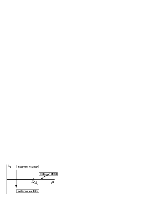
Figure 2: A schematic phase diagram. The thick line in the abscissa is the line of critical points discussed in the test. All regions except the thin line in the abscissa are in the instanton insulator phase. A scan along the line with an arrow will exhibit the closing of the absorption gap when cross the abscissa.

To study the Rabi oscillation in the instanton metal phase we need to compute the $P(t)$ in Eq. (5) in the presence of an environment. To do it non-perturbatively we connect it to the correlation functions of the Ising model. Let $|0\rangle$ be the ground state of Eq. (3). The initial observation of $\tau_{z}=+1$ projects the state of the system to $\left(1+\tau_{z}\over 2\right)|0\rangle.$ Using the time evolution operator associated with Eq. (3) to evolve this state and computing the $\tau_{z}$ expectation value at a later time $t$ we obtain

$$P(t) ={1\over 2\langle 0|1+\tau_{z}|0\rangle}\{\langle 0|\tau_{z}(t)|0\rangle+\langle 0|\tau_{z}\tau_{z}(t)\tau_{z}|0\rangle$$ (23)

$$+\langle 0|\tau_{z}\tau_{z}(t)|g\rangle+\langle 0|\tau_{z}(t)\tau_{z}|g\rangle\},$$

where $\tau_{z}(t)=e^{iHt}\tau_{z}e^{-iHt}$. It is important to note that in the above equation $t$ is the real (not imaginary) time. At $\Delta_{0}=0$ and in the absence of spontaneous symmetry breaking $\langle 0|\tau_{z}(t)|0\rangle=\langle 0|\tau_{z}\tau_{z}(t)\tau_{z}|0\rangle=0$. As a result

$$P(t)=\langle 0|\tau_{z}\tau_{z}(t)|g\rangle+\langle 0|\tau_{z}(t)\tau_{z}|g\rangle=\int_{0}^{\infty}\cos(\omega t)A(\omega)d\omega.$$ (24)

Inserting Eq. (19) into Eq. (24), we calculated the Rabi oscillation in the instanton metal phase, the result is presented in Fig.1(b). One can see a damped Rabi oscillations qualitative similar to the perturbative result shown in Fig.1(a). In the instanton insulator phase, the strong coupling with the environment locks the the two-level-cavity system, and the Rabi oscillations is complectly quenched.

In summary, we have shown that although the environment is harmful to quantum coherence, it contains interesting physics in its own right. In particular, we have demonstrated that when the environment is Ohmic and only causes dephasing, there is a quantum phase transition between a state which exhibits damped Rabi oscillation to a state which does not. In reality the dephasing-only requirement of our model has been achieved partially already in experiment. For example, for the “Cooper pair box” a $T_{1}$ (life time due to the up $\leftrightarrow$ down flipping of the two-level system) which is an order of magnitude longer than $T_{2}$ (the dephasing life time) has been achieved siddiqi . In the langauge of Ising model, $T_{1}/\tau_{0}$ imposes a finite size cutoff to the critical behavior discussed earlier. Hopefully future technological progresses will enable one to probe the regime where $T_{1}>>T_{2}$, hence the novel 1D analog of the Kosterlitz-Thouless critical behavior.

- (1) J. M. Raimond, M. Brune, and S. Haroche, Rev. Mod. Phys. 73, 565 (2001).
- (2) H. Mabuchi, and A. C. Doherty, Science 298, 1372 (2002).
- (3) T. H. Stievater et al., Phys. Rev. Lett. 87, 133603 (2001).
- (4) A. Wallraff et al., Nature 431, 162 (2004); ibid. 431, 159 (2004).
- (5) K.-J. Boller, A. Imamoglu, and S. E. Harris, Phys. Rev. Lett. 66, 2593 (1991).
- (6) M. Fleischhauser, A. Imamoglu, and J. P. Marangos, Rev. Mod. Phys. 77, 633 (2005).
- (7) A. J. Leggett et al., Rev. Mod. Phys. 59, 1 (1987).
- (8) M. I. Dykman and M. A. Krivoglaz, Sov. Phys. Solid State 29, 210 (1987).
- (9) B. W. Shore and P. L. Knight, J. Mod. Opt. 40, 1195 (1993).
- (10) A. O. Caldeira and A. J. Leggett, Phys. Rev. Lett.46, 211 (1981); Ann. Phys.(N.Y.) 149, 374 (1983).
- (11) R. de Sousa et al., Phys. Rev. Lett. 95 247006 (2005).
- (12) C. Q. Wu, J. X. Li, and D. H. Lee, cond-mat/0612202 (unpublished).
- (13) E. Luijten and H. MeBingfeld, Phys. Rev. Lett. 86, 5305 (2001).
- (14) I. Siddiqi et al., Phys. Rev. B 73, 054510 (2006).