Parallel Self-Consistent-Field Calculations via Chebyshev-Filtered Subspace Acceleration

Abstract

Solving the Kohn-Sham eigenvalue problem constitutes the most computationally expensive part in self-consistent density functional theory (DFT) calculations. In a previous paper, we have proposed a nonlinear Chebyshev-filtered subspace iteration method, which avoids computing explicit eigenvectors except at the first SCF iteration. The method may be viewed as an approach to solve the original nonlinear Kohn-Sham equation by a nonlinear subspace iteration technique, without emphasizing the intermediate linearized Kohn-Sham eigenvalue problems. It reaches self-consistency within a similar number of SCF iterations as eigensolver-based approaches. However, replacing the standard diagonalization at each SCF iteration by a Chebyshev subspace filtering step results in a significant speedup over methods based on standard dagonalization. Here, we discuss an approach for implementing this method in multi-processor, parallel environment. Numerical results are presented to show that the method enables to perform a class of highly challenging DFT calculations that were not feasible before.

I Introduction

Electronic structure calculations based on first principles use a very successful combination of density functional theory (DFT) hkohn:64 ; kosh:65 and pseudopotential theory phillips-58 ; phil-klein-59 ; chelik-cohen-92 ; martin_book_04 . DFT reduces the original multi-electron Shrödinger equation into an effective one-electron Kohn-Sham equation, where all non-classical electronic interactions are replaced by a functional of the charge density. The pseudopotential theory further simplifies the problem by replacing the true atomic potential with an effective “pseudopotential” that is smoother but takes into account the effect of core electrons. Combining pseudopotential with DFT greatly reduces the number of one-electron wave-functions to be computed. However, even with these simplifications, solving the final Kohn-Sham equation can still be computationally challenging, especially when the systems being studied are complex or contain thousands of atoms.

Several approaches have been employed in solving the Kohn-Sham equations. They can be classified in two major groups: basis-free or basis-dependent approaches, according to whether they use an explicit basis set for electronic orbitals or not. Among the basis-dependent approaches, plane-wave methods are frequently used in applications of DFT to periodic systems payne:92 ; vasp96 , whereas localized basis sets are very popular in quantum-chemistry applications martin_book_04 ; koch_book_00 . Special basis sets, which do not make use of pseudopotentials, have also been designed for all-electron DFT calculations. These basis sets include localized atomic orbitals, linearized augmented plane waves, muffin-tin orbitals, and projector-augmented waves. A survey of advantages and disadvantages of these explicit-basis methods can be found in martin_book_04 . Real-space methods are basis-free, and they have gained ground in recent years cts:94 ; ctws:94 ; real-space-cg ; beck-00 due in great part to their simplicity. One advantage of real-space methods is that they are quite easy to implement in parallel environment. A second advantage is that, in contrast with the plane-wave approach, they do not impose artificial periodicity in non-periodic systems. Third, the application of potentials onto electron wave-functions is performed directly in real space. Although the Hamiltonian matrices with a real-space approach are typically larger than with plane waves, the Hamiltonians are highly sparse and never stored or computed explicitly. Only matrix-vector products that represent the application of the Hamiltonians on wave-functions need to be computed.

This article focusses on effective techniques to handle the most computationally expensive part of DFT calculations, namely the self-consistent-field (SCF) iteration. We present details of a recently developed nonlinear Chebyshev-filtered subspace iteration (CheFSI) method. The sequential version of CheFSI is first proposed in chefsi . The parallel CheFSI is implemented in our own DFT package called PARSEC (Pseudopotential Algorithm for Real-Space Electronic Calculations) cts:94 ; ctws:94 . Although CheFSI is described in the framework of real-space DFT, the subspace filtering method can be employed to other Self-Consistent Field iterations. This method takes advantage of the fact that intermediate SCF iterations do not require accurate eigenvalues and eigenvectors of the Kohn-Sham equation.

The Standard SCF iteration framework is used in CheFSI, and a self-consistent solution is sought, which means that CheFSI has the same accuracy as other standard DFT approaches. One can view CheFSI as a technique to directly tackle the original nonlinear Kohn-Sham eigenvalue problems by a form of nonlinear subspace iteration, without emphasizing the intermediate linearized Kohn-Sham eigenvalue problems. In fact, within CheFSI, explicit eigenvectors are computed only at the first SCF iteration, in order to provide a suitable initial subspace. After the first SCF step, the explicit computation of eigenvectors at each SCF iteration is replaced by a single subspace filtering step. The method reaches self-consistency within a number of SCF iterations that is close to that of eigenvector-based approaches. However, since eigenvectors are not explicitly computed after the first step, a significant gain in execution time results when compared with methods based on explicit diagonalization. When compared with calculations based on efficient eigenvalue packages such as ARPACK lesy:98 and TRLan trlan99 ; wusi:00 , a tenfold or higher speed-up is usually observed. CheFSI enabled us to perform a class of highly challenging DFT calculations, including clusters with over ten thousand atoms, which were not feasible before.

This article begins with a summary of SCF for DFT calculations in Section II. Details about the parallel implementation are included in Section III. The Chebyshev subspace filtering algorithm is presented in Section IV, and the block Chebyshev-Davidson algorithm for the initial diagonalization is discussed in Section V. The block Chebyshev-Davidson method chebydav ; bdavio improves considerably the efficiency of the diagonalization at the first SCF iteration, compared with the thick-restart Lanczos (TRLan) method trlan99 ; wusi:00 which was used in chefsi . The paper ends with numerical results in Section VI, and a few concluding remarks.

II Eigenvalue problems in DFT SCF calculations

Within DFT, the multi-electron Schrödinger equation is simplified as the following Kohn-Sham equation:

$$\left[-\frac{\hbar^{2}}{2M}\nabla^{2}+V_{total}(\rho(r),r)\right]\Psi_{i}(r)=E_{i}\Psi_{i}(r),$$ (1)

where $\Psi_{i}(r)$ is a wave function, $E_{i}$ is a Kohn-Sham eigenvalue, $\hbar$ is the Planck constant, and $M$ is the electron mass. In practice we use atomic units, thus $\hbar=M=1$.

The total potential $V_{total}$, also referred to as the effective potential, includes three terms,

$$V_{total}(\rho(r),r)=V_{ion}(r)+V_{H}(\rho(r),r)+V_{XC}(\rho(r),r),$$ (2)

where $V_{ion}$ is the ionic potential, $V_{H}$ is the Hartree potential, and $V_{XC}$ is the exchange-correlation potential.

The Hartree and exchange-correlation potentials depend on the charge density $\rho(r)$, which is defined as

$$\rho(r)=2\sum_{i=1}^{n_{occ}}|\Psi_{i}(r)|^{2}.$$ (3)

Here $n_{occ}$ is the number of occupied states, which is equal to half the number of valence electrons in the system. The factor of two comes from spin multiplicity. Equation (3) can be easily extended to situations where the highest occupied states have fractional occupancy or when there is an imbalance in the number of electrons for each spin component.

The most computationally expensive step of DFT is in solving the Kohn-Sham equation 1. Since $V_{total}$ depends on the charge density $\rho(r)$, which in turn depends on the wavefunctions $\Psi_{i}$, this equation can be viewed as a nonlinear eigenvalue problem. The SCF iteration is a general technique used to solve this nonlinear eigenvalue problem. It starts with an initial guess of the charge density, then obtains the initial $V_{total}$ and solves 1 for $\Psi_{i}(r)$’s to update $\rho(r)$ and $V_{total}$. Then 1 is solved again for the new $\Psi_{i}(r)$’s and the process is iterated until $V_{total}$ (and also the wave functions) becomes stationary.

In general, most of the computational effort involved in DFT is spent solving equation 1. For this reason, it is the goal of any DFT code to lessen the burden of solving 1 in the SCF iteration. One possible avenue to achieve this is to use better diagonalization routines. However this approach is limited as most diagonalization software has now reached maturation. At the other extreme, one can attempt to avoid diagonalization altogether, and this leads to the body of work represented by linear-scaling or order-N methods (see e.g. goed99 ). This approach however has other limitations. In particular, the approximations involved rely heavily on some decay properties of the density matrix in certain function bases. In particular, they will be difficult to implement in real-space discretizations. Our approach lies somewhere between these extremes. We take advantage of the fact that accurate eigenvectors are unnecessary at each SCF iteration, since Hamiltonians are only approximate in the intermediate SCF steps, and we exploit the nonlinear nature of the problem. The main point of our algorithm, developed in chefsi , is that once we have a good starting point for the Hamiltonian, it suffices to filter each basis vector at each iteration. In the intermediate SCF steps, these vectors are no longer eigenvectors but together they represent a good basis of the desired invariant subspace. The parallel implementation of the idea will be discussed in Section IV. The next section summarizes parallel implementation issues in PARSEC.

III The parallel environment in PARSEC

PARSEC uses pseudopotential real-space implementation of DFT. The motivation and original ideas behind the method go back to the early 1990s cts:94 ; ctws:94 . Within PARSEC, an uniform Cartesian grid in real-space is placed on the region of interest, and the Kohn-Sham equation is discretized by a high order finite-difference method fd-acta94 on this grid. Wavefunctions are expressed as functions of grid positions. Outside a specified sphere boundary that encloses the physical system, wavefunctions are set to zero for non-periodic systems. In addition to the advantages mentioned in the introduction, another advantage of the real-space approach is that periodic boundary conditions are also reasonably simple to implement wjkc:04 .

The latest version of PARSEC is written in Fortran 95. PARSEC has now evolved into a mature, massively parallel package, which includes most of the functionality of comparable DFT codes parsec-k . The reader is referred to Saad-al-Elec ; sosck:00 for details and the rationale of the parallel implementation. The following is a brief summary of the most important points.

The parallel mode of PARSEC uses the standard Message Passing Interface (MPI) library for communication. Parallelization is achieved by partitioning the physical domain which can have various shapes depending on boundary conditions and symmetry operations. Figure 1 illustrates four cube-shaped neighboring sub-domains. For a generic, confined system without symmetry, the physical domain is a sphere which contains all atoms plus some additional space (due to delocalization of electron charge). In recent years, PARSEC has been enhanced to take advantage of physical symmetry. If the system is invariant upon certain symmetry operations, the physical domain is replaced with an irreducible wedge constructed according to those operations. For example, if the system has mirror symmetry on the $xy$ plane, the irreducible wedge covers only one hemisphere, either above or below the mirror plane. For periodic systems, the physical domain is the periodic cell, or an irreducible wedge of it if symmetry operations are present. In any circumstance, the physical domain is partitioned in compact regions, each assigned to one processor only. Good load balance is ensured by enforcing that the compact regions have approximately the same number of grid points.

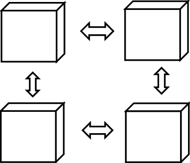
Figure 1: Sample decomposition of a physical domain in PARSEC.

Once the physical domain is partitioned, the physical problem is mapped onto the processors in a data-parallel way: each processor is in charge of a block of rows of the Hamiltonian corresponding to the block of grid points assigned to it. The eigenvector and potential vector arrays are row-wise distributed in the same fashion. The program only requires an index function $indx(i,j,k)$ which returns the number of the processor in which the grid point $(i,j,k)$ resides.

Because the Hamiltonian matrix is never stored, we need an explicit reordering scheme which renumbers rows consecutively from one processor to the next one. For this purpose we use a list of pointers that gives for each processor, the row with which it starts.

Since finite difference discretizetion is used, when performing an operation such as a matrix-vector product, communication will be required between nearest neighbor processors. For communication we use two index arrays, one to count how many and which rows are needed from neighbors, the other to count the number of local rows needed by neighbors.

With this design of decomposition and mapping, the data required by the program can be completely distributed. Being able to distribute the memory requirement is quite important in solving large problems on standard supercomputers.

Parallelizing subspace methods for the linearized eigenvalue problems (obtained from a finite difference discretization of eqn. 1) becomes quite straightforward with the above mentioned decomposition and mapping. Note that the subspace basis vectors contain approximations to eigenvectors, therefore the rows of the basis vectors are distributed in the same way as the rows of the Hamiltonian. All matrix-matrix products, matrix-vector products, and vector updates (e.g., linear combinations of vectors), can be executed in parallel.

Reduction operations, e.g., computing inner products and making the result available in each processor, are efficiently handled by the MPI reduction function MPI_ALLREDUCE().

IV The nonlinear Chebyshev-filtered subspace iteration

The main idea of CheFSI is to start with a good initial subspace $V$ corresponding to occupied states of the initial Hamiltonian. This initial $V$ is usually obtained by a diagonalization step. No diagonalizations are necessary after the first SCF step. Instead, the subspace from the previous iteration is filtered by a low degree-$m$ Chebyshev polynomial, $p_{m}(t)$, constructed for the current Hamiltonian $H$. The polynomial differs at each SCF step since $H$ changes. The goal of the filter is to make the subspace spanned by $p_{m}(H)V$ approximate the eigensubspace corresponding to the occupied states of the final $H$. At the intermediate SCF steps, the basis need not be an accurate eigenbasis since the intermediate Hamiltonians are not exact. The filtering is designed so that the resulting sequence of subspaces will progressively approximate the desired eigensubspace of the final Hamiltonian when self-consistency is reached.

Our approach exploits the well-known fast growth property outside the $[-1,1]$ interval of the Chebyshev polynomial, this allows us to use low degree Chebyshev polynomials to achieve sufficient filtering. At each SCF step, only two parameters are required to construct an effective Chebyshev filter, namely, a lower bound and an upper bound of the higher portion of the spectrum of the current Hamiltonian $H$ in which we want $p_{m}(t)$ to be small. We propose simple but efficient ways to obtain these bounds, very little additional cost is required for the bound estimates.

After self-consistency is reached, the Chebyshev filtered subspace includes the eigensubspace corresponding to occupied states. Explicit eigenvectors can be readily obtained by a Rayleigh-Ritz refinement parlet:98 (also called subspace rotation) step.

We refer to chefsi ; tr-pchefsi for more algorithmic details and a literature survey concerning application of Chebyshev polynomials in DFT calculations.

The main structure of the CheFSI method is given in Algorithm IV.1. It is quite similar to that of the standard SCF iteration discussed in Section II. One major difference is that the inner iteration for diagonalization at Step 2 is now performed only at the first SCF step. Thereafter, diagonalization is replaced by a single Chebyshev-Filtered Subspace step, denoted as CheFS in Algorithm IV.1.

Algorithm IV.1

CheFSI for SCF calculation:
    1.  Start from an initial guess of $\rho(r)$, get  $V_{total}(\rho(r),r)$.   2.  Solve  $\left[-\frac{1}{2}{\nabla^{2}}+V_{total}(\rho(r),r)\right]\Psi_{i}(r)=E_{i}\Psi_{i}(r)$   for $\Psi_{i}(r),\;i=1,2,...,s$.   3.  Compute new charge density  $\rho(r)=2\sum_{i=1}^{n_{occ}}|\Psi_{i}(r)|^{2}$.   4.  Solve for new Hartree potential  $V_{H}$ from   $\nabla^{2}V_{H}(r)=-4\pi\rho(r)$.   5.  Update  $V_{XC}$; get new  ${\tilde{V}}_{total}(\rho,r)=V_{ion}(r)+V_{H}(\rho,r)+V_{XC}(\rho,r)$ with
a potential-mixing step.   6.  If  $\|{\tilde{V}}_{total}-V_{total}\|<tol$, stop.   7.  $V_{total}\leftarrow{\tilde{V}}_{total}$ (update $H$ implicitly); apply the following
Chebyshev-Filtered Subspace (CheFS) method to get $s$ approximate wavefunctions: 7.1)  Compute  $b_{up}:=$ upper bound of the spectrum of $H$
Set $b_{low}:=$ the largest Ritz value from previous iteration. 7.2)  Perform Chebyshev filtering to the matrix $\Psi$, whose column-vectors
are the $s$ discretized wavefunctions of $\Psi_{i}(r),~{}i=1,...,s$:
$$\Psi={\tt Chebyshev\_filter}(\Psi,~{}m,~{}b_{low},~{}b_{up})~{},$$ 7.3)  Ortho-normalize the basis $\Psi$ by iterated Gram-Schmidt. 7.4)  Perform the Rayleigh-Ritz (rotation) step: a) Compute $\hat{H}=\Psi^{T}H\Psi$; b) Compute the eigendecomposition of $\hat{H}$:  $\hat{H}Q=QD$,
where $D$ contains non-increasingly ordered eigenvalues of $\hat{H}$,
and $Q$ contains the corresponding eigenvectors; c) ’Rotate’ the basis as $\Psi:=\Psi Q$;  return $\Psi$ and $D$.   8.  Goto step 3.  

The upper bound at step 7.1 in Algorithm IV.1 can be obtained by using an upper-bound-estimator presented in chefsi . The Chebyshev-filter step in step 7.2 calls a subroutine which applies the Chebyshev filter to each of the columns of $\Psi$. If $m$ is the degree of the polynomial, this operation amounts to computing the sequence of blocks $X_{k}$, $k=2,\cdots,m$ as follows:

$$X_{k+1}={2\over e}(H-cI)X_{k}-X_{k-1},\quad k=1,2,\cdots,m-1$$

starting with $X_{0}=\Psi$, $X_{1}={1\over e}(H-cI)X_{0}$. The returned filtered block is $\Psi=X_{m}$. The scalars $e$ and $c$ are defined by $e=(b_{up}-b_{low})/2$ and $c=(b_{up}+b_{low})/2$. For simplicity we presented here an unscaled version of the filtering process. To prevent the $X_{k}$ blocks from overflowing it is safer to scale them at each iteration. The scaling operation is inexpensive as it uses only values of the Chebyshev polynomial at the approximate smallest eigenvalue of the Hamiltonian. The reader is referred to chefsi for details. For discussion of scaling related to Chebyshev filtering, we refer interested readers to chebydav or a more detailed technical report tr-pchefsi .

The parallel implementation of Algorithms IV.1 is straightforward with the parallel paradigm discussed in Section III. We only mention that the matrix-vector products related to filtering, computing upper bounds, and Rayleigh-Ritz refinement, can easily be executed in parallel. The re-orthogonalization at Step 7.3  of Algorithm IV.1 uses a parallel version of the iterated Gram-Schmidt DGKS method dgks:76 , which scales better than the standard modified Gram-Schmidt algorithm.

The estimated complexity of the algorithm is similar to that of the sequential CheFSI method in chefsi . For parallel computation it suffices to estimate the complexity on a single processor. Assume that $p$ processors are used, i.e., each processor shares $N/p$ rows of the full Hamiltonian. The estimated cost of a CheFS step on each processor with respect to the dimension of the Hamiltonian denoted by $N$, and the number of computed states $s$, is as follows:

• The Chebyshev filtering in Step 7.2 costs $O(s*N/p)$ flops. The discretized Hamiltonian is sparse and each matrix-vector product on one processor costs $O(N/p)$ flops. Step 7.2 requires $m*s$ matrix-vector products, at a total cost of $O(s*m*N/p)$ where the degree $m$ of the polynomial is small (typically between 8 and 20).

• The ortho-normalization in Step 7.3 costs $O(s^{2}*N/p)$ flops. There are additional communication costs because of the global reductions.

• The eigen-decomposition at Step 7.4 costs $O(s^{3})$ flops.

• The final basis refinement step ($\Psi:=\Psi Q$) costs $O(s^{2}*N/p)$.

If a standard iterative diagonalization method is used to solve the eigenproblem 1 at each SCF step, then it also requires (i) the orthonormalization of a (typically larger) basis; (ii) the eigen-decomposition of the projected Rayleigh-quotient matrix; and (iii) the basis refinement (rotation). These operations need to be performed several times within this single diagonalization. But CheFS performs each of these operations only once per SCF step. Therefore, although CheFS scales in a similar way to standard diagonalization-based methods, the scaling constant is much smaller. For large problems, CheFS can achieve a tenfold or more speedup per SCF step, over using the well-known efficient eigenvalue packages such as ARPACK lesy:98 and TRLan trlan99 ; wusi:00 . The total speedup can be more significant since self-consistency requires several SCF iteration steps.

To summarize, a standard SCF method would have an outer SCF loop—the usual nonlinear SCF loop, and an inner diagonalization loop, which iterates until eigenvectors are within specified accuracy. Algorithm IV.1 simplifies this by merging the inner-outer loops into a single outer loop, which can be considered as a nonlinear subspace iteration algorithm. The inner diagonalization loop is reduced into a single Chebyshev subspace filtering step.

V Chebyshev-Davidson algorithm for the first SCF iteration

Within CheFSI, the most expensive SCF step is the first one, as it involves a diagonalization in order to compute a good initial subspace to be used for latter filtering. In principle, any effective eigenvalue algorithms can be used. PARSEC originally had three diagonalization methods: Diagla, which is a preconditioned Davidson method Saad-al-Elec ; sosck:00 ; the symmetric eigensolver in ARPACK sorens:92 ; lesy:98 ; and the Thick-Restart Lanczos algorithm called TRLan trlan99 ; wusi:00 . For systems of moderate sizes, Diagla works well, and then becomes less competitive relative to ARPACK or TRLan for larger systems when a large number of eigenvalues are required. TRLan is about twice as fast as the symmetric eigensolver in ARPACK, because of its reduced need for re-orthogonalization. In chefsi , TRLan was used for the diagonalization at the first SCF step.

For very large systems, memory can become a severe constraint. One has to use eigenvalue algorithms with restart since out-of-core operations can be too slow. However, even with standard restart methods such as ARPACK and TRLan, the memory demand can still surpass the capacity of some supercomputers. For example, the $Si_{9041}H_{1860}$ cluster by TRLan or ARPACK would require more memory than the largest memory allowed for a job at the Minnesota Supercomputing Institute in 2006. Hence it is important to develop a diagonalization method that is less memory demanding but whose efficiency is comparable to ARPACK and TRLan. The Chebyshev-Davidson method chebydav ; bdavio is developed with these two goals in mind.

It is generally accepted that for the implicit filtering in ARPACK and TRLan to work efficiently, one needs to use a subspace with dimension about twice the number of wanted eigenvalues. This leads to a relatively large demand in memory when the number of wanted eigenvalues is large. The block Chebyshev-Davidson method discussed in bdavio introduced an inner-outer restart technique. The outer restart corresponds to a standard restart in which the subspace is truncated to a smaller dimension when the specified maximum subspace dimension is reached. The inner restart corresponds to a standard restart restricted to an active subspace, it is performed when the active subspace dimension exceeds a given integer $act_{max}$ which is much smaller than the specified maximum subspace dimension. With inner-outer restart, the subspace used in Chebyshev-Davidson is about half the dimension of the subspace required by ARPACK or TRLan.

We adapted the proposed Chebyshev filters into a Davidson-type eigenvalue algorithm. Although no Ritz values are available from previous SCF steps to be used as lower bounds, the Rayleigh-Ritz refinement step within a Davidson-type method can easily provide a suitable lower bound at each iteration. The upper bound is again estimated by the upper-bound-estimator in chefsi , and it is computed only once. These two bounds are sufficient for constructing a filter at each Chebyshev-Davidson iteration. The constructed filter magnifies the wanted lower end of the spectrum and dampens the unwanted higher end, therefore the filtered block of vectors have strong components in the wanted eigensubspace, which results in an efficiency that is comparable to that of ARPACK or TRLan. The main structure of this Chebyshev-Davidson method is sketched in Algorithm V.1, we refer interested readers to bdavio for algorithmic details.

Algorithm V.1

Structure outline of the block Chebyshev-Davidson method
    1.  Compute  ${b_{up}}$ using the upper-bound-estimator in chefsi ;  set  ${b_{low}}$ as the median of the
eigenvalues of the tri-diagonal matrix from the upper-bound-estimator.
Make the given initial size-$k$ block $V_{1}$ orthonormal, set $V=[V_{1}]$.   2.  $[~{}V_{f}~{}]={{\tt Chebyshev\_filter}}(V_{1},m,{b_{low},b_{up}})$.   3.  Augment the basis $V$ by $V_{f}$:  $V\leftarrow\left[~{}V,~{}{V_{f}}~{}\right]$, make $V$ orthonormal.   4.  Inner-restart if active subspace dimension exceeds a given integer  $act_{max}$.   5.  Rayleigh-Ritz refinement:  update matrix $M$ s.t.  $M=V^{T}HV$;
do eigendecomposition of $M$:  $M~{}Y=YD$;  updated basis $V$:  $V\leftarrow V\ Y$.   6.  Compute residual vectors, determine convergence;
perform deflation if some eigenpairs converge.   7.  If all wanted eigenpairs converged, stop;  else, adapt ${b_{low}}=max(diag(D))$,
set  $V_{1}=$ $[$ the first $k$ non-converged Ritz vectors in $V$ $]$.   8.  Outer-restart if size of  $V$ exceeds maximum subspace dimension.   9.  Continue from step 2.  

The first step diagonalization by the block Chebyshev-Davidson method, together with the Chebyshev-filtered subspace (CheFS) method, enabled us to perform SCF calculations for a class of large systems, including the silicon cluster $Si_{9041}H_{1860}$ for which over 19000 eigenvectors of a Hamiltonian with dimension around 3 million were to be computed. These systems are practically infeasible with the other three eigensolvers (ARPACK, TRLan and Diagla) in PARSEC, using the current supercomputer resources available to us at the Minnesota Supercomputing Institute (MSI).

VI Numerical Results

PARSEC has been applied to study a wide range of material systems (e.g. wjkc:04 ; parsec-k ; ctws:94 ). The focus of this section is on large systems where relatively few numerical results exist because of the infeasibility of eigenvector-based methods. We mention that zhaoy-04 contains very interesting studies on clusters containing up to 1100 silicon atoms, using the well-known efficient plane-wave DFT package VASP kres-haf94 ; vasp96 ; however, it is stated in zhaoy-04 that a cluster with 1201 silicon atoms is “too computationally intensive”. As a comparison, PARSEC using CheFSI, together with the currently developed symmetric operations of real-space pseudopotential methods tiago_unpub , can now routinely solve silicon clusters with several thousand atoms.

The hardware used for the computations is the SGI Altix cluster at MSI, it consists of 256 Intel Itanium processors at CPU rates of 1.6 GHz, sharing 512 GB of memory (but a single job is allowed to request at most 250 GB memory).

The goal of the computations is not to study the parallel scalability of PARSEC, but rather to use PARSEC to do SCF calculation for large systems that were not studied before. Therefore we do not use different processor numbers to solve the same problem. Scalability is studied in sosck:00 for the preconditioned Davidson method. Here we mention that the scalability of CheFS is better than eigenvector-based methods because of the reduced reorthogonalizations.

sysem	dim. of $H$	$n_{state}$	#MVp	#SCF	total_eV/atom	1st CPU	total CPU
$Si_{2713}H_{828}$ a	1074080	5843	1400187	14	-86.16790	7.83 hrs.	19.56 hrs.
$Si_{4001}H_{1012}$ b	1472440	8511	1652243	12	-89.12338	18.63 hrs.	38.17 hrs.
$Si_{6047}H_{1308}$ c	2144432	12751	2682749	14	-91.34809	45.11 hrs.	101.02 hrs.
$Si_{9041}H_{1860}$ d	2992832	19015	4804488	18	-92.00412	102.12 hrs.	294.36 hrs
$Fe_{302}$ e	2790688	$1812\times 2$	9377435	110	-795.18064	16.16 hrs.	112.44 hrs.
$Fe_{326}$ f	2985992	$1956\times 2$	10241385	119	-795.19898	11.62 hrs.	93.15 hrs.
$Fe_{360}$ g	3262312	$2160\times 2$	12989799	146	-795.22329	16.55 hrs.	140.68 hrs.

^a $m=10$ for CheFS. First step diagonalization by TRLan cost 8.65 hours, projecting it into a 14-steps SCF iteration cost around 121.1 hours.

Table 1: Performance of the CheFSI method in various test systems. All calculations were performed using 16 processors, and polynomial degrees $m=17$ for the Chebyshev-Davidson and $m=8$ for CheFSI, except when otherwise stated.

In the reported numerical results, the total_eV/atom is the total energy per atom in electron-volts, this value can be used to assess accuracy of the final result; the #SCF is the iteration steps needed to reach self-consistency; and the #MVp counts the number of matrix-vector products. Clearly #MVp is not the only factor that determines CPU time, the orthogonalization cost can also be a significant component.

For all of the reported results for CheFSI, the first step diagonalization used the Chebyshev-Davidson method (Algorithm V.1). In Table 1, the 1st CPU denotes the CPU time spent on the first step diagonalization by Chebyshev-Davidson; the total CPU counts the total CPU time spent to reach self-consistency by CheFSI.

method	#MVp	#SCF steps	total_eV/atom	CPU(secs)
CheFSI	189755	11	-77.316873	542.43
TRLan	149418	10	-77.316873	2755.49
Diagla	493612	10	-77.316873	8751.24

Table 2: $Si_{525}H_{276}$, using 16 processors. The Hamiltonian dimension is 292584, where 1194 states need to be computed at each SCF step. The first step diagonalization by Chebyshev-Davidson cost 79755 #MVp and 221.05 CPU seconds; so the total #MVp spent on CheFS in CheFSI is 110000. The polynomial degree used is $m=17$ for Chebyshev-Davidson and $m=8$ for CheFS. The fist step diagonalization by TRLan requires 14909 #MVp and 265.75 CPU seconds.

The first example in Table 1 is a relatively small silicon cluster $Si_{525}H_{276}$, which is used to compare the performance of CheFSI with two eigenvector-based methods. All methods use the same symmetry operations tiago_unpub in PARSEC.

For larger clusters $Si_{2713}H_{828}$ and $Si_{4001}H_{1012}$ , Diagla became too slow to be practical. However, we could still apply TRLan for the first step diagonalization for comparison, but we did not iterate until self-consistency was reached since that would cost a significant amount of our CPU quota. Note that with the problem size increasing, Chebyshev-Davidson compares more favorably over TRLan. This is because we employed an additional trick in Chebyshev-Davidson, which corresponds to allowing the last few eigenvectors not to converge to the required accuracy. The number of the non fully converged eigenvectors is bounded above by $act_{max}$, which is the maximum dimension of the active subspace. Typically $30\leq act_{max}\leq 300$ for Hamiltonian size over a million where several thousand eigenvectors are to be computed. The implementation of this trick is rather straightforward since it corresponds to applying the CheFS method to the subspace spanned by the last few vectors in the basis that have not converged to required accuracy.

For even larger clusters $Si_{6047}H_{1308}$ and $Si_{9041}H_{1860}$, it became impractical to apply TRLan for the first step diagonalization because of too large memory requirements. For these large systems, using an eigenvector-based method for each SCF step is clearly not feasible. We note that the cost for the first step diagonalization by Chebyshev-Davidson is still rather high, it took close to 50% of the total CPU. In comparison, the CheFS method saves a significant amount of CPU for SCF calculations over diagonalization-based methods, even if very efficient eigenvalue algorithms are used.

Once the DFT problem, Eq. (1), is solved, we have access to several physical quantities. One of them is the ionization potential (IP) of the nanocrystal, defined as the energy required to remove one electron from the system. Numerically, we use a $\Delta SCF$ method: perform two separate calculations, one for the neutral cluster and another for the ionized one, and observe the variation in total energy between these calculations. Figure 2 shows the IP of several clusters, ranging from the smallest possible ($SiH_{4}$) to $Si_{9041}H_{1860}$. For comparison, we also show the eigenvalue of the highest occupied Kohn-Sham orbital, $E_{HOMO}$. A known fact of DFT-LDA is that the negative of the $E_{HOMO}$ energy is lower than the IP in clusters martin_book_04 , which is confirmed in Figure 2. In addition, the figure shows that the IP and $-E_{HOMO}$ approach each other in the limit of extremely large clusters.

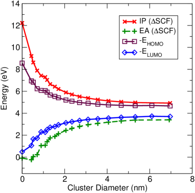
Figure 2: Ionization potential (IP, crosses) and electron affinity (EA, “plus” signs) for various clusters with diameters ranging from 0 nm ($SiH_{4}$) to 7 nm ($Si_{9041}H_{1860}$). Squares denote the negative of the highest occupied eigenvalue energy ($-E_{HOMO}$) of the neutral cluster. Diamonds denote the negative of the lowest unoccupied eigenvalue energy ($-E_{LUMO}$).

Figure 2 also shows the electron affinity (EA) of the various clusters. The EA is defined as the energy released by the system when one electron is added to it. Again, we calculate it by performing SCF calculations for the neutral and the ionized systems (negatively charged instead of positively charged now). In PARSEC, this sequence of SCF calculations can be done very easily by reusing previous information: The initial diagonalization in the second SCF calculation is waived if we reuse eigenvectors and eigenvalues from a previous calculation as initial guesses for the ChebFSI method. Figure 2 shows that, as the cluster grows in size, the EA approaches the negative of the lowest-unoccupied eigenvalue energy. A power-law analysis in Figure 2 indicates that both the ionization potential and the electron affinity approach their bulk values according to a power-law decay $R^{n}$ with exponent close to 1. The numerical fits are:

$${\rm IP}={\rm IP}_{0}+A/D^{\alpha}$$ (4)

$${\rm EA}={\rm EA}_{0}-B/D^{\beta}$$ (5)

with ${\rm IP}_{0}=$ 4.50 eV, ${\rm EA}_{0}=$ 3.87 eV, $\alpha=$ 1.16, $\beta=$ 1.09, $A=$ 3.21 eV, $B=$ 3.13 eV. These values for $A$ and $B$ assume a cluster diameter $D$ given in nanometers. The difference between ionization potential and electron affinity is the electronic gap of the nanocrystal. As expected, the value of the gap extrapolated to bulk, ${\rm IP}_{0}-{\rm EA}_{0}=$ 0.63 eV, is very close to the energy gap predicted in various DFT calculations for silicon, which range from 0.6 eV to 0.7 eV martin_book_04 ; aulbur00 . Owing to the slow power-law decay, the gap at the largest crystal studied is still 0.7 eV larger than the extrapolated value.

Other properties of large silicon clusters are also expected to be similar to the ones of bulk silicon, which is equivalent to a nanocrystal of “infinite size”. Figure 3 shows that the density of states already assumes a bulk-like profile in clusters with around ten thousand atoms. The presence of hydrogen atoms on the surface is responsible for subtle features in the DOS at around -8 eV and -3 eV. Because of the discreteness of eigenvalues in clusters, the DOS is calculated by adding up normalized Gaussian distributions located at each calculated energy eigenvalue. In Figure 3, we used Gaussian functions with dispersion of 0.05 eV. More details are discussed in silicon-parsec .

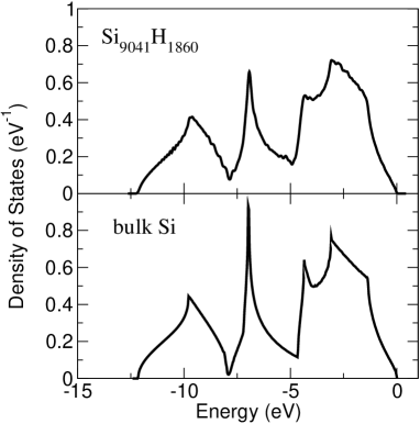
Figure 3: Density of states (DOS) of the cluster $Si_{9041}H_{1860}$ (upper panel) compared with periodic crystalline silicon (lower panel). As a consequence of the large size, the DOS of the $Si_{9041}H_{1860}$ cluster is very close to that of bulk silicon (the infinite-size limit).

We also applied PARSEC to some large iron clusters. Extensive analysis of the magnetic properties of iron clusters based on the methodology presented here and in previous workchefsi , has provided decisive evidence for surface effects in the magnetic moment of these systems iron-parsec , confirming earlier experimental data. Table 1 also contains three clusters with more than 300 iron atoms. These metallic systems are well-known to be very difficult for DFT calculations, because of the “charge sloshing” payne:92 ; vasp96 . The LDA approximation used to get exchange-correlation potential $V_{XC}$ is also known not to work well for iron atoms. However, PARSEC was able to reach self-consistency for these large metallic clusters within reasonable time length. It took more than 100 SCF steps to reach self-consistency, which is generally considered too high for SCF calculations, but we observed (from calculations performed on smaller iron clusters) that eigenvector-based methods also required a similar number of SCF steps to converge, thus the slow convergence is associated with the difficulty of DFT for metallic systems. Without CheFS, and under the same hardware conditions as listed in Table 1, over 100 SCF steps using eigenvector-based methods would have required months to complete for each of these clusters.

VII Concluding Remarks

We developed and implemented the parallel CheFSI method for DFT SCF calculations. Within CheFSI, only the first SCF step requires a true diagonalization, and we perform this step by the block Chebyshev-Davidson method. No diagonalization is required after the first step; instead, Chebyshev filters are adaptively constructed to filter the subspace from previous SCF steps so that the filtered subspace progressively approximates the eigensubspace corresponding to occupied states of the final Hamiltonian. The method can be viewed as a nonlinear subspace iteration method which combines the SCF iteration and diagonalization, with the diagonalization simplified into a single step Chebyshev subspace filtering.

Additional tests not reported here, have also shown that the subspace filtering method is robust with respect to the initial subspace. Besides self-consistency, it can be used together with molecular dynamics or structural optimization, provided that atoms move by a small amount. Even after atomic displacements of a fraction of the Bohr radius, the CheFSI method was able to bring the initial subspace to the subspace of self-consistent Kohn-Sham eigenvectors for the current position of atoms, with no substantial increase in the number of self-consistent cycles needed.

CheFSI significantly accelerates the SCF calculations, and this enabled us to perform a class of large DFT calculations that were not feasible before by eigenvector-based methods. As an example of physical applications, we discuss the energetics of silicon clusters containing up to several thousand atoms.

- (1) P. Hohenberg and W. Kohn, Phys. Rev. 136, B864 (1964).
- (2) W. Kohn and L. J. Sham, Phys. Rev. 140, A1133 (1965).
- (3) J. C. Phillips, Phys. Rev. 112, 685 (1958).
- (4) J. C. Phillips and L. Kleinman,Phys. Rev. 116, 287 (1959).
- (5) J. R. Chelikowsky and M. L. Cohen, Handbook on Semiconductors, volume 1, p.59. (Elsevier, Amsterdam, 1992).
- (6) R. M. Martin, Electronic structure : Basic theory and practical methods. Electronic structure : Basic theory and practical methods ( Cambridge University Press, 2004).
- (7) M. C. Payne, M. P. Teter, D. C. Allan, T. A. Arias, and J. D. Joannopoulos, Rev. Mod. Phys. 64, 1045 (1992).
- (8) G. Kresse and J. Furthmüller, Phys. Rev. B 54, 11169 (1996).
- (9) W. Koch and M. C. Holthausen, A chemist’s guide to density functional theory ( Wiley-VCH, 2000).
- (10) J. R. Chelikowsky, N. Troullier, and Y. Saad, Phys. Rev. Lett. 72, 1240 (1994).
- (11) J. R. Chelikowsky, N. Troullier, K. Wu, and Y. Saad, Phys. Rev. B 50, 11355 (1994).
- (12) A. P. Seitsonen, M. J. Puska, and R. M. Nieminen, Phys. Rev. B 51, 14057 (1995).
- (13) T. L. Beck, Rev. Mod. Phys. 72, 1041 (2000).
- (14) Y. Zhou, Y. Saad, M. L. Tiago, and J. R. Chelikowsky, J. Comput. Phys. (in press).
- (15) R. B. Lehoucq, D. C. Sorensen, and C. Yang, ARPACK USERS GUIDE: Solution of Large Scale Eigenvalue Problems by Implicitly Restarted Arnoldi Methods (SIAM, Philadelphia, 1998). Available at http//www.caam.rice.edu/software/ARPACK/.
- (16) K. Wu, A. Canning, H. D. Simon, and L.-W. Wang, J. Comput. Phys. 154, 156 (1999).
- (17) K. Wu and H. Simon, SIAM J. Matrix Anal. Appl. 22, 602 (2000).
- (18) Y. Zhou and Y. Saad, Technical report, Minnesota Supercomputing Institute, Univ. of Minnesota, (in revision).
- (19) Y. Zhou, Technical report, Minnesota Supercomputing Institute, Univ. of Minnesota, (in revision).
- (20) S. Goedecker, Rev. Mod. Phys. 71, 1085 (1999).
- (21) B. Fornberg and D. M. Sloan, Acta Numerica, editor A. Iserles, number 3, p. 203. (Cambridge Univ. Press, 1994).
- (22) M. M. G. Alemany, M. Jain, L. Kronik, and J. R. Chelikowsky, Phys. Rev. B 69, 075101 (2004).
- (23) L. Kronik, A. Makmal, M. Tiago, M. Alemany, M. Jain, X. Huang, Y. Saad, and J. Chelikowsky, Phys. Status Solidi B 243, 1063 (2006).
- (24) Y. Saad, A. Stathopoulos, J. Chelikowsky, K. Wu, and S. Öğüt, BIT 36, 563 (1996).
- (25) A. Stathopoulos, S. Öğüt, Y. Saad, J.R. Chelikowsky, and H. Kim, IEEE Computing in Science and Engineering 2, 19 (2000).
- (26) B. N. Parlett, The Symmetric Eigenvalue Problem, Number 20 in Classics in Applied Mathematics (SIAM, Philadelphia, PA, 1998).
- (27) Y. Zhou, Y. Saad, M. L. Tiago, and J. R. Chelikowsky, Technical report, Minnesota Supercomputing Institute, Univ. of Minnesota, 2006
- (28) J. Daniel, W. B. Gragg, L. Kaufman, and G. W. Stewart, Math. Comp. 30, 772 (1976).
- (29) D. C. Sorensen, SIAM J. Matrix Anal. Appl. 13, 357 (1992).
- (30) Y. Zhao, M.-H. Du Y.-H. Kim, and S.B. Zhang, Phys. Rev. Lett. 93, 015502 (2004).
- (31) G. Kresse and J. Hafner, J. Phys.: Condens. Matter 6, 8245 (1994).
- (32) M. L. Tiago and J. R. Chelikowsky, Technical report, Univ. Texas, Austin, (in preparation).
- (33) W. G. Aulbur, L. Jönsson, and J. W. Wilkins, Solid State Physics, eds. F. Seitz, D. Turnbull, and H. Ehrenreich, vol. 54, 1, Academic, New York (2000).
- (34) M. L. Tiago, Y. Zhou, Y. Saad, and J. R. Chelikowsky, Technical report.
- (35) M. L. Tiago, Y. Zhou, M. M. G. Alemany, Y. Saad, and J. R. Chelikowsky, Phys. Rev. Lett. 97, 147201 (2006).