The multi-configurational time-dependent Hartree method for bosons: Many-body dynamics of bosonic systems

Abstract

The evolution of Bose-Einstein condensates is amply described by the time-dependent Gross-Pitaevskii mean-field theory which assumes all bosons to reside in a single time-dependent one-particle state throughout the propagation process. In this work, we go beyond mean-field and develop an essentially-exact many-body theory for the propagation of the time-dependent Schrödinger equation of $N$ interacting identical bosons. In our theory, the time-dependent many-boson wavefunction is written as a sum of permanents assembled from orthogonal one-particle functions, or orbitals, where both the expansion coefficients and the permanents (orbitals) themselves are time-dependent and fully determined according to a standard time-dependent variational principle. By employing either the usual Lagrangian formulation or the Dirac-Frenkel variational principle we arrive at two sets of coupled equations-of-motion, one for the orbitals and one for the expansion coefficients. The first set comprises of first-order differential equations in time and non-linear integro-differential equations in position space, whereas the second set consists of first-order differential equations with time-dependent coefficients. We call our theory multi-configurational time-dependent Hartree for bosons, or MCTDHB($M$), where $M$ specifies the number of time-dependent orbitals used to construct the permanents. Numerical implementation of the theory is reported and illustrative numerical examples of many-body dynamics of trapped Bose-Einstein condensates are provided and discussed.

I Introduction

The experimental realizations of Bose-Einstein condensates made of ultracold alkali-metal atoms Wieman_Cornell_Science_1995 ; Ketterle_PRL_1995 ; Ketterle_Nobel_lecture ; Cornell_Wieman_Nobel have stimulated a modern renaissance as to possible utilization of cold trapped atoms and Bose-Einstein condensates, for instance to quantum information processing Cirac_Zoller_1995 ; Brennen_PRL_quan_comp_1999 and interferometric-based precession measurements Orzel , and to the fundamental physics governing trapped interacting bosons Leggett_review ; Pethich_book ; Stringari_book . An ultimate goal of researchers is to be able to design, realize, manipulate and detect desired quantum states of the many-atom system.

Static and dynamical properties of Bose-Einstein condensates have been extensively and successfully explored in the community by employing the mean-field Gross-Pitaevskii theory GPO1 ; GPO2 , for reviews see Leggett_review ; Pethich_book ; Stringari_book and for individual applications to condensates and mixtures R1 ; R2 ; R3 ; R4 ; R5 ; R6 ; R7 and BB_Ho ; BB_Esry ; BB_Pu ; r21 ; r22 ; r23 , respectively. Gross-Pitaevskii theory is an excellent theory for weakly-interacting bosons whenever a single macroscopic one-particle wavefunction is sufficient to describe the reality. By definition, Gross-Pitaevskii theory cannot describe phenomena such as fragmentation of condensates or Mott-insulator phases in optical lattices for which two, few or many one-particle functions are occupied. Recently, we have developed a multi-orbital mean-field approach to describe static and dynamical properties of fragmented condensates LA_PLA ; OAL_PLA_2007 , thus generalizing the (one-orbital) Gross-Pitaevskii mean-field. Utilizing the multi-orbital mean-field has enabled us to find new phenomena associated with fragmentation, fermionization, quantum phases, demixing scenarios and interferences of interacting bosonic systems in traps and optical lattices u1 ; u2 ; u3 ; u4 ; u5 .

In spite the great successes and popularity of mean-field approaches in the many-boson problem of degenerate quantum gases, the need and demand for practical many-body theoretical approaches and computational tools is widely accepted and well documented, see, e.g., the review numerical_review and references therein. Nowadays, finite-number condensates can be produced (and reliably reproduced) in experiments. For instance, see the work of the Raizen group which demonstrated atom-number squeezing with as little as a few tens of atoms Raizen_SQ , and the experiment of the Oberthaler group which demonstrated a single Josephson junction in a double-well with a few thousands of atoms Oberthaler_JJ . Experiments as those call for delicate description of beyond mean-field, finite-particle-number, and many-body effects.

The purpose of the present work is to develop an essentially-exact and numerically-efficient time-dependent approach for the solution of the time-dependent many-boson Schrödinger equation. Recently, we have developed a general variational theory with complete self-consistency for studying stationary properties of condensates in traps on a quantitative many-body level MCHB_paper . The main idea of Ref. MCHB_paper is the computation of the best (optimal) stationary many-body wavefunctions expressed as a linear combination of permanents. In reminiscence to our approach in the stationary many-boson problem MCHB_paper , we will here optimize the time-dependent many-body wavefunctions according to a time-dependent variational principle. We term our approach multi-configurational time-dependent Hartree for bosons (MCTDHB). The equations-of-motion of MCTDHB have been recently posted in their final form in Ref. ramp_up_Letter , where we employed MCTDHB to the popular problem of splitting a Bose-Einstein condensate by deforming a single well to a double-well. Applying MCTDHB to the ramping-up-a-barrier problem we followed the many-boson wavefunction throughout the splitting process and identified the role and impact of many-body excited-states on the splitting process. Among others, we were able to identify a new ’counter-intuitive’ regime where the evolution of the condensate when the barrier in ramped-up sufficiently slow is not to the ground-state of the double-well which is a fragmented condensate, but to a low-lying excited-state which is a coherent condensate ramp_up_Letter . Here we provide the derivation of the MCTDHB theory, details of the numerical implementation of MCTDHB, and complementary illustrative numerical examples.

Evidences that employing time-dependent orbitals (permanents) in attacking the time-dependent many-boson Scrördinger equation beyond Gross-Pitaevskii theory is useful and important have already appeared in the literature. Zoller and co-workers addressed the ramping-up-a-barrier problem with two time-dependent orbitals of Gaussian shape whose positions and phase change in time t2 . More recently, Masiello and Reinhardt have used a time-dependent multi-configurational ansatz with two orbitals of predetermined gerade and ungerade symmetries to describe interferences in a symmetric double-well set-up MR_2007 . In this context, we would like to stress that MCTDHB is fully variational and is not restricted to the number of orbitals, to a predetermined shape or symmetry of the orbitals, and to the geometry, dimensionality and interparticle interactions of the time-dependent many-boson problem.

It is instructive to place the MCTDHB theory developed and presented in this paper in the general context of multi-configurational time-propagation approaches of many-particle systems. The idea to expand and optimize the time-dependent many-body wavefunction of distinguishable particles is long known and termed multi-configurational time-dependent self-consistent field approach Makri ; Kosloff1 ; Kosloff2 . A particular efficient variant of the multi-configurational time-dependent self-consistent field approach is the multi-configuration time-dependent Hartree (MCTDH) approach which has been successfully and routinely used for multi-dimensional dynamical systems consisting of distinguishable particles CPL ; JCP ; CMF ; PR .

The MCTDH approach can treat efficiency and accurately static and dynamical properties of a few-particle systems. In the latter context, we mention that very recently static properties of weakly- to strongly-interacting trapped few-boson systems have been studied on a quantitative many-body level by MCTDH ZP1 ; ZP2 . Yet, in treating a larger number of identical particles it is essential to use their statistic properties to truncate the large amount of redundancies of coefficients in the distinguishable-particle multi-configurational expansion of the MCTDH wavefunction. In this case, the challenge was first approached for fermionic systems where a fermionic version of MCTDH was independently developed by several groups MCTDHF1 ; MCTDHF2 ; MCTDHF3 , taking explicitly the antisymmetry of the many-fermion wavefunction to permutations of any two particles into account.

Here we accept the respective challenge for bosons. This is in particular valuable since very-many bosons can reside in only a small number of orbitals. Alternatively speaking, by explicitly exploiting bosons’ statistics it is possible to successfully and quantitatively attack the dynamics of a much large number of bosons with the present MCTDHB theory. A second importance difference in comparison with MCTDH is the nature of interparticle interactions. In MCTDHB we employ a general two-body interaction between identical bosons whereas MCTDH was designated to treat nuclear dynamics in which interactions normally involve several degrees-of-freedom, or coordinates.

The structure of the paper is as follows. In section II we develop the working equations of MCTDHB, highlighting their appealing representation in terms of reduced one- and two-body densities and discussing properties of MCTDHB. In section III we present details of the numerical implementation of MCTDHB. Illustrative numerical examples are provided in section IV, whereas summary and conclusions are given in section V. Finally, complementary material is differed to appendices A and B.

II Theory

The evolution of $N$ interacting structureless bosons is governed by the time-dependent Schrödinger equation:

$$\hat{H}\Psi=i\frac{\partial\Psi}{\partial t},\qquad\hat{H}({\bf r}_{1},{\bf r}_{2},\ldots,{\bf r}_{N})=\sum_{j=1}^{N}\hat{h}({\bf r}_{j})+\sum_{k>j=1}^{N}W({\bf r}_{j}-{\bf r}_{k}).$$ (1)

Here $\hbar=1$, ${\bf r}_{j}$ is the coordinate of the $j$-th boson, $\hat{h}({\bf r})=\hat{T}({\bf r})+V({\bf r})$ is the one-body Hamiltonian containing kinetic and potential energy terms, and $W({\bf r}_{j}-{\bf r}_{k})$ describes the pairwise interaction between the $j$-th and $k$-th bosons. In the most general case, the one-body potential $V({\bf r})$ and the two-body interaction $W({\bf r}_{j}-{\bf r}_{k})$ and, hence, the many-boson Hamiltonian $\hat{H}$ itself may be time-dependent. To avoid cumbersome notation in what follows, we do not indicate explicitly this time-dependence unless it is necessary.

The time-dependent many-boson Schrödinger equation (1) cannot be solved exactly (analytically), except for a few specific cases only, see, e.g., Ref. Marvin . Hence, theoretical and numerical strategies for attacking this problem are a must.

II.1 Derivation of the working equations of MCTDHB

We would like to start by constructing a formally-exact representation of the time-dependent many-boson wavefunction $\Psi(t)$ describing the dynamics of $N$ identical structureless bosons. To this end and following the Introduction part, we allow the bosons to occupy permanents made of time-dependent one-particle functions, or orbitals. Let us introduce a complete set of time-dependent orbitals $\left\{\phi_{k}({\bf r},t)\right\}$ which are normalized and orthogonal to one another at any time $t$,

$$\int\phi^{\ast}_{k}({\bf r},t)\phi_{j}({\bf r},t)d{\bf r}=\delta_{kj}.$$ (2)

In what follows, it is convenient to work in second quantization formalism and introduce the set of bosonic annihilation operators corresponding to the orbitals $\left\{\phi_{k}({\bf r},t)\right\}$. This is conveniently done by employing the relation,

$$b_{k}(t)=\int\phi_{k}^{\ast}({\bf r},t)\hat{\mathbf{\Psi}}({\bf r})d{\bf r},$$ (3)

where $\hat{\mathbf{\Psi}}({\bf r})=\sum_{k}b_{k}(t)\phi_{k}({\bf r},t)$ is the usual bosonic field operator annihilating a particle at position ${\bf r}$. The bosonic annihilation and corresponding creation operators obey the usual commutation relations $b_{k}(t)b^{\dagger}_{j}(t)-b^{\dagger}_{j}(t)b_{k}(t)=\delta_{kj}$ at any time. Using the creation operators $b^{\dagger}_{k}(t)$ we assemble the permanents,

$$\left|\vec{n};t\right>=\frac{1}{\sqrt{n_{1}!n_{2}!n_{3}!\cdots n_{M}!}}\left(b_{1}^{\dagger}(t)\right)^{n_{1}}\left(b_{2}^{\dagger}(t)\right)^{n_{2}}\cdots\left(b_{M}^{\dagger}(t)\right)^{n_{M}}\left|vac\right>,$$ (4)

where $\vec{n}=(n_{1},n_{2},n_{3},\cdots,n_{M})$ represents the occupations of the orbitals that preserve the total number of particles $n_{1}+n_{2}+n_{3}+\cdots+n_{M}=N$, $M$ is a number of the one-particle functions, and $\left|vac\right>$ is the vacuum.

In the multi-configuration time-dependent Hartree approach for bosons (MCTDHB) the ansatz for the many-body wavefunction $\Psi(t)$ is taken as a linear combination of time-dependent permanents (4) ramp_up_Letter ,

$$\left|\Psi(t)\right>=\sum_{\vec{n}}C_{\vec{n}}(t)\left|\vec{n};t\right>,$$ (5)

where the summation runs over all possible configurations whose occupations $\vec{n}$ preserve the total number of bosons $N$. Of course, in the limit $M\to\infty$ the set of permanents $\{\left|\vec{n};t\right>\}$ spans the complete $N$-boson Hilbert space and thus expansion (5) is exact. So where is the advantage of utilizing an expansion with time-dependent permanents? In practice, we have of course to limit the size of the Hilbert space exploited in computations. Now, by allowing also the permanents to be time-dependent we can use much shorter expansions than if only the expansion coefficients are taken to be time-dependent, thus leading to a significant computational advantage. We would like to highlight that in representation (5) both the expansion coefficients $\{C_{\vec{n}}(t)\}$ and orbitals $\{\phi_{k}({\bf r},t)\}$ comprising the permanents $\left|\vec{n};t\right>$ are independent parameters. To solve for the time-dependent wavefunction $\Psi(t)$ means to determine the evolution of the coefficients $\{C_{\vec{n}}(t)\}$ and orbitals $\{\phi_{k}({\bf r},t)\}$ in time.

To derive the equations-of motion governing the evolution of $\{C_{\vec{n}}(t)\}$ and $\{\phi_{k}({\bf r},t)\}$ we need to employ a time-dependent variational principle. Two such variational principles are utilized here, both leading to the same result, of course, but highlighting complementary aspects when treating the time-dependent many-boson problem. Specifically, in the bulk of the paper below we employ the usual Lagrangian formulation LF1 ; LF2 , whereas how to derive the MCTDHB equations-of-motion starting from the Dirac-Frenkel variational principle DF1 ; DF2 is deferred to appendix B. The main difference between the two (equivalent) formulations employed here is that, in the Lagrangian formulation we are to take first expectation values and only subsequently perform the variation which somewhat simplifies the algebra, whereas in the Dirac-Frenkel formulation the situation reverses, i.e., variation of $\Psi(t)$ precedes the computation of matrix elements.

In the framework of the Lagrangian formulation LF1 ; LF2 , we substitute the many-body ansatz (5) for $\Psi(t)$ into the functional action of the time-dependent Schrödinger equation which reads:

$$S\left[\{C_{\vec{n}}(t)\},\{\phi_{k}({\bf r},t)\}\right]=\int dt\left\{\left<\Psi\left|\hat{H}-i\frac{\partial}{\partial t}\right|\Psi\right>-\sum_{k,j}^{M}\mu_{kj}(t)\left[\left<\phi_{k}|\phi_{j}\right>-\delta_{kj}\right]\right\}.$$ (6)

The time-dependent Lagrange multipliers $\mu_{kj}(t)$ are introduced to ensure that the time-dependent orbitals $\phi_{k}({\bf r},t)$ remain orthonormal throughout the propagation, see (2) and appendix B. The next step is to require stationarity of the action with respect to its arguments $\{C_{\vec{n}}(t)\}$ and $\{\phi_{k}({\bf r},t)\}$. This variation is performed below separately for the coefficients and for the orbitals, recalling that they are independent variational parameters.

II.1.1 Variation with respect to the expansion coefficients $\{C_{\vec{n}}(t)\}$

To take the variation of the functional action (6) with respect to the expansion coefficients $\{C_{\vec{n}}(t)\}$ we first express the expectation value in the action in a form which explicitly depends on the expansion coefficients,

$$\left<\Psi\left|\hat{H}-i\frac{\partial}{\partial t}\right|\Psi\right>=\sum_{\vec{n}}C^{\ast}_{\vec{n}}\left[\sum_{\vec{n}^{\prime}}\left<\vec{n};t\left|\hat{H}-i\frac{\partial}{\partial t}\right|\vec{n}^{\prime};t\right>C_{\vec{n}^{\prime}}-i\frac{\partial C_{\vec{n}}}{\partial t}\right].$$ (7)

It is now straightforward to perform this variation which gives,

$$\frac{\partial S\left[\{C_{\vec{n}}(t)\},\{\phi_{k}({\bf r},t)\}\right]}{\partial C^{\ast}_{\vec{n}}(t)}=0\qquad\Longrightarrow\qquad\sum_{\vec{n}^{\prime}}\left<\vec{n};t\left|\hat{H}-i\frac{\partial}{\partial t}\right|\vec{n}^{\prime};t\right>C_{\vec{n}^{\prime}}=i\frac{\partial C_{\vec{n}}}{\partial t}.$$ (8)

Defining the time-dependent matrix $\mbox{\boldmath$\mathcal{H}$}(t)$ the elements of which are

$${\mathcal{H}}_{\vec{n}\vec{n}^{\prime}}(t)=\left<\vec{n};t\left|\hat{H}-i\frac{\partial}{\partial t}\right|\vec{n}^{\prime};t\right>,$$ (9)

and collecting the expansion coefficients $C_{\vec{n}}(t)$ in the column vector ${\bf C}(t)$, Eq. (8) can be written in a compact matrix form as:

$$\mbox{\boldmath$\mathcal{H}$}(t){\bf C}(t)=i\frac{\partial{\bf C}(t)}{\partial t}.$$ (10)

Let us discuss the properties of Eq. (10). The equation-of-motion (10) is a first-order differential equation in time. The matrix $\mbox{\boldmath$\mathcal{H}$}(t)$ multiplying the vector ${\bf C}(t)$ on the left-hand-side is time-dependent, since it is evaluated with time-dependent permanents $\left|\vec{n};t\right>$ and $\left|\vec{n}^{\prime};t\right>$, comprised themselves of time-dependent orbitals.

In the course of evolution, the many-body wavefunction $\Psi(t)$ should, of course, remain normalized since for self-adjoined Hamiltonians $\hat{H}$ the evolution is unitary. $\left|\Psi(t)\right>=\sum_{\vec{n}}C_{\vec{n}}(t)\left|\vec{n};t\right>$ would remain normalized if the vector of coefficients ${\bf C}(t)$ remains normalized in time throughout propagation via Eq. (10) (the orbitals comprising the permanents remain orthonormal to one another by virtue of the Lagrange multipliers, see subsection II.1.2 for more details). For this, the matrix $\mbox{\boldmath$\mathcal{H}$}(t)$ should be hermitian.

Below, we first evaluate the matrix $\mbox{\boldmath$\mathcal{H}$}(t)$ explicitly and then show that it is always hermitian. Derivation of the rules to evaluate matrix elements of one- and two-body operators between two general permanents can be found in MCHB_paper . Here the matrix elements with respect to two general time-dependent permanents $\left|\vec{n};t\right>$ and $\left|\vec{n}^{\prime};t\right>$ are displayed in their final form. Noticing that in second quantization the time-derivative can be treated as a one-body operator,

$$i\frac{\partial}{\partial t}=\sum_{k,q}b_{k}^{\dagger}b_{q}\left(i\frac{\partial}{\partial t}\right)_{kq},$$ (11)

the non-vanishing matrix elements of the one-body operator $\hat{h}-i\frac{\partial}{\partial t}$ are given by

$$\left<\vec{n};t\left|\hat{h}-i\frac{\partial}{\partial t}\right|\vec{n};t\right>=\sum_{l=1}^{M}n_{l}\left[h_{ll}-\left(i\frac{\partial}{\partial t}\right)_{ll}\right],$$

$$\left<\vec{n}_{q}^{k};t\left|\hat{h}-i\frac{\partial}{\partial t}\right|\vec{n};t\right>=\sqrt{(n_{k}+1)n_{q}}\left[h_{kq}-\left(i\frac{\partial}{\partial t}\right)_{kq}\right],\ k\neq q,\$$ (12)

where the permanent denoted by $\left|\vec{n}_{q}^{k};t\right>$ differs from $\left|\vec{n};t\right>$ by an excitation of one boson from the $q$-th to the $k$-th orbital. The corresponding matrix elements of the two-body operator $\hat{W}$ between two permanents $\left|\vec{n};t\right>$ and $\left|\vec{n}^{\prime};t\right>$ are collected for convenience in appendix A. The time-dependent matrix elements of the one- and two-body operators with respect to orbitals needed in this work are given by:

$$h_{kq} = \int\phi_{k}^{\ast}({\bf r},t)\hat{h}({\bf r})\phi_{q}({\bf r},t)d{\bf r},$$

$$\left(i\frac{\partial}{\partial t}\right)_{kq} = i\int\phi_{k}^{\ast}({\bf r},t)\frac{\partial\phi_{q}({\bf r},t)}{\partial t}d{\bf r},$$

$$W_{ksql} = \int\!\!\int\phi_{k}^{\ast}({\bf r},t)\phi_{s}^{\ast}({\bf r}^{\prime},t)\hat{W}({\bf r}-{\bf r}^{\prime})\phi_{q}({\bf r},t)\phi_{l}({\bf r}^{\prime},t)d{\bf r}d{\bf r}^{\prime},$$

$$W_{ks[ql]} = W_{ksql}+W_{kslq}.$$ (13)

Note the plus sign in $W_{ks[ql]}$ which is due to bosons’ statistics.

With the elements of $\mbox{\boldmath$\mathcal{H}$}(t)$ explicitly expressed, we can return now to the question of its hermiticity. Clearly, the contribution originating from the matrix elements of the Hamiltonian, $h_{kq}$ and $W_{ksql}$, is hermitian for any set of of functions $\{\phi_{k}({\bf r},t)\}$ belonging to the domain of the Hamiltonian. To show that the matrix representation of $i\frac{\partial}{\partial t}$ is also hermitian we make use of the fact that the orbitals $\{\phi_{k}({\bf r},t)\}$ are kept normalized and orthogonal to one another at any time. Taking the time derivative of Eq. (2) we readily get

$$i\frac{\partial}{\partial t}\left[\int\phi^{\ast}_{k}({\bf r},t)\phi_{q}({\bf r},t)d{\bf r}\right]=0\quad\Longrightarrow\quad\left(i\frac{\partial}{\partial t}\right)_{kq}=\left(i\frac{\partial}{\partial t}\right)^{\ast}_{qk}.$$ (14)

Summarizing, we have shown that the matrix ${\mbox{\boldmath$\mathcal{H}$}}(t)$ is hermitian for a general set of orbitals $\{\phi_{k}({\bf r},t)\}$ that are kept normalized and orthogonal to one another at any time. Consequently, the evolution of the expansion coefficients $\{C_{\vec{n}}(t)\}$ is always unitary, namely, that an initially normalized expansion coefficient vector ${\bf C}(t)$ propagated by Eq. (10) remains normalized at any time. This result, together with Eq. (2), guarantees that an initially normalized many-body state $\Psi(0)$ remains normalized at any time.

II.1.2 Variation with respect to the orbitals $\{\phi_{k}({\bf r},t)\}$

In the present subsection we derive the equations-of-motion governing the evolution of the orbitals $\{\phi_{k}({\bf r},t)\}$. Now, it is helpful to express the expectation value of $\hat{H}-i\frac{\partial}{\partial t}$ appearing in the functional action (6) in a form which allows one for a direct functional differentiation with respect to $\phi_{k}({\bf r},t)$.

To this end, we write the operator $\hat{H}-i\frac{\partial}{\partial t}$ in second quantization form:

$$\hat{H}-i\frac{\partial}{\partial t}=\sum_{k,q}b_{k}^{\dagger}b_{q}\left[h_{kq}-\left(i\frac{\partial}{\partial t}\right)_{kq}\right]+\frac{1}{2}\sum_{k,s,q,l}b_{k}^{\dagger}b_{s}^{\dagger}b_{q}b_{l}W_{ksql},$$ (15)

where the matrix elements of the one- and two-body operators are given in Eq. (II.1.1). In calculating the expectation value of (15) with respect to the many-boson wavefunction $\Psi(t)$ it is gratifying to make use of the one- and two-body density matrices $\rho_{kq}(t)=\left<\Psi\left|b_{k}^{\dagger}b_{q}\right|\Psi\right>$ and $\rho_{ksql}(t)=\left<\Psi\left|b_{k}^{\dagger}b_{s}^{\dagger}b_{q}b_{l}\right|\Psi\right>$, respectively. Given the (normalized) wavefunction $\Psi(t)$, the one-body density matrix is given by

$$\rho({\bf r}_{1}|{\bf r}^{\prime}_{1};t) = N\int\Psi^{\ast}({\bf r}^{\prime}_{1},{\bf r}_{2},\ldots,{\bf r}_{N};t)\Psi({\bf r}_{1},{\bf r}_{2},\ldots,{\bf r}_{N};t)d{\bf r}_{2}d{\bf r}_{3}\cdots d{\bf r}_{N}=$$ (16)

$$= \left<\Psi(t)\left|\hat{\mathbf{\Psi}}^{\dagger}({\bf r}^{\prime}_{1})\hat{\mathbf{\Psi}}({\bf r}_{1})\right|\Psi(t)\right>=\sum^{M}_{k,q=1}\rho_{kq}(t)\phi^{\ast}_{k}({\bf r}^{\prime}_{1},t)\phi_{q}({\bf r}_{1},t),\$$

where the matrix elements of the density explicitly read

$$\rho_{kk}(t)=\sum_{\vec{n}}C_{\vec{n}}^{\ast}C_{\vec{n}}n_{k},$$

$$\rho_{kq}(t)=\sum_{\vec{n}}C_{\vec{n}}^{\ast}C_{\vec{n}_{k}^{q}}\sqrt{n_{k}(n_{q}+1)},\ k\neq q.\$$ (17)

It is convenient to collect these matrix elements as $\mbox{\boldmath$\rho$}(t)=\left\{\rho_{kq}(t)\right\}$. Similarly, the two-body density matrix associated with $\Psi(t)$ is given by

$$\!\!\!\rho({\bf r}_{1},{\bf r}_{2}|{\bf r}^{\prime}_{1},{\bf r}^{\prime}_{2};t)=N(N-1)\int\Psi^{\ast}({\bf r}^{\prime}_{1},{\bf r}^{\prime}_{2},{\bf r}_{3},\ldots,{\bf r}_{N};t)\Psi({\bf r}_{1},{\bf r}_{2},{\bf r}_{3},\ldots,{\bf r}_{N};t)d{\bf r}_{3}\cdots d{\bf r}_{N}=$$

$$\!\!\!=\left<\Psi(t)\left|\hat{\mathbf{\Psi}}^{\dagger}({\bf r}^{\prime}_{1})\hat{\mathbf{\Psi}}^{\dagger}({\bf r}^{\prime}_{2})\hat{\mathbf{\Psi}}({\bf r}_{1})\hat{\mathbf{\Psi}}({\bf r}_{2})\right|\Psi(t)\right>=\sum^{M}_{k,s,q,l=1}\rho_{ksql}(t)\phi^{\ast}_{k}({\bf r}^{\prime}_{1},t)\phi^{\ast}_{s}({\bf r}^{\prime}_{2},t)\phi_{q}({\bf r}_{1},t)\phi_{l}({\bf r}_{2},t),$$

where the matrix elements $\rho_{ksql}$ are collected for convenience in appendix A.

Combining the above ingredients we obtain for the expectation value of the operator $\hat{H}-i\frac{\partial}{\partial t}$ appearing in the factional action (6),

$$\left<\Psi\left|\hat{H}-i\frac{\partial}{\partial t}\right|\Psi\right>=\sum_{k,q=1}^{M}\rho_{kq}\left[h_{kq}-\left(i\frac{\partial}{\partial t}\right)_{kq}\right]+\frac{1}{2}\sum_{k,s,q,l=1}^{M}\rho_{ksql}W_{ksql}-i\sum_{\vec{n}}C^{\ast}_{\vec{n}}\frac{\partial C_{\vec{n}}}{\partial t}.$$ (19)

Note the appealing appearance of representation (19) in which the only explicit dependence on the orbitals $\{\phi_{k}({\bf r},t)\}$ is grouped into the matrix elements $h_{kq},\,\left(i\frac{\partial}{\partial t}\right)_{kq}$ and $W_{ksql}$ of the one- and two-body operators $\hat{h}-i\frac{\partial}{\partial t}$ and $\hat{W}$, respectively, whereas the elements $\rho_{kq}$ and $\rho_{ksql}$ of the density matrices do not depend explicitly on the orbitals. Consequently, it is now straightforward to perform variation of the functional action (6) with respect to the orbitals $\{\phi_{k}({\bf r},t)\}$ which gives the following set of coupled equations-of-motion, $k=1,\ldots,M$,

$$\frac{\delta S\left[\{C_{\vec{n}}(t)\},\{\phi_{k}({\bf r},t)\}\right]}{\delta\phi^{\ast}_{k}({\bf r},t)}=0\ \ \Longrightarrow\ \ \sum^{M}_{q=1}\left[\rho_{kq}\left(\hat{h}-i\frac{\partial}{\partial t}\right)+\sum^{M}_{s,l=1}\rho_{ksql}\hat{W}_{sl}\right]\left|\phi_{q}\right>=\sum^{M}_{j=1}\mu_{kj}\left|\phi_{j}\right>,$$ (20)

where

$$\hat{W}_{sl}({\bf r},t)=\int\phi_{s}^{\ast}({\bf r}^{\prime},t)W({\bf r}-{\bf r}^{\prime})\phi_{l}({\bf r}^{\prime},t)d{\bf r}^{\prime}$$ (21)

are local time-dependent potentials.

To proceed, we can use the constraints (2) that the $\phi_{k}({\bf r},t)$ are functions orthonormal to one another in order to eliminate the Lagrange multipliers $\mu_{kj}(t)$ from Eq. (20). By taking the scalar product of $\left<\phi_{j}\right|$ with (20), the resulting $\mu_{kj}(t)$ take on the form,

$$\mu_{kj}(t)=\sum^{M}_{q=1}\left\{\rho_{kq}\left[h_{jq}-\left(i\frac{\partial}{\partial t}\right)_{jq}\right]+\sum^{M}_{s,l=1}\rho_{ksql}W_{jsql}\right\}.$$ (22)

Substituting Eq. (22) into (20), employing the identities

$$\sum^{M}_{q=1}\left[\rho_{kq}\left(\hat{h}-i\frac{\partial}{\partial t}\right)+\sum^{M}_{s,l=1}\rho_{ksql}\hat{W}_{sl}\right]\left|\phi_{q}\right>-\sum^{M}_{j=1}\mu_{kj^{\prime}}\left|\phi_{j}^{\prime}\right>=$$

$$\left(1-\sum_{j^{\prime}=1}^{M}\left|\phi_{j^{\prime}}\left>\right<\phi_{j^{\prime}}\right|\right)\sum^{M}_{q=1}\left[\rho_{kq}\left(\hat{h}-i\frac{\partial}{\partial t}\right)+\sum^{M}_{s,l=1}\rho_{ksql}\hat{W}_{sl}\right]\left|\phi_{q}\right>,\quad k=1,\ldots,M,$$ (23)

and multiplying from the left with the inverse of the one-body density and summing over $\sum_{k}\left\{\mbox{\boldmath$\rho$}(t)\right\}^{-1}_{jk}$, we arrive immediately at the following form of the equations-of-motion of the orbitals $\phi_{j}({\bf r},t)$, $j=1,\ldots,M$:

$$\hat{\mathbf{P}}i\left|\dot{\phi}_{j}\right>=\hat{\mathbf{P}}\left[\hat{h}\left|\phi_{j}\right>+\sum^{M}_{k,s,q,l=1}\left\{\mbox{\boldmath$\rho$}(t)\right\}^{-1}_{jk}\rho_{ksql}\hat{W}_{sl}\left|\phi_{q}\right>\right],$$

$$\qquad\hat{\mathbf{P}}=1-\sum_{j^{\prime}=1}^{M}\left|\phi_{j^{\prime}}\left>\right<\phi_{j^{\prime}}\right|.\$$ (24)

Here and hereafter we use the shorthand notation $\dot{\phi}_{j}\equiv\frac{\partial\phi_{j}}{\partial t}$. Examining Eq. (II.1.2) we see that eliminating the Lagrange multipliers $\mu_{kj}(t)$ has emerged as a projection operator $\hat{\mathbf{P}}$ onto the subspace orthogonal to that spanned by the $\{\phi_{k}({\bf r},t)\}$. This projection appears both on the left- and right-hand-sides of (II.1.2), making (II.1.2) a cumbersome coupled system of integro-differential non-linear equations.

Fortunately, due to the invariance properties of the ansatz (5), see discussion in subsection II.2 below, we can always perform a unitary transformation without introducing further constraints on the orbitals such that CPL ; JCP

$$\left<\phi_{k}|\dot{\phi}_{q}\right>=0,\ \ k,q=1,\ldots,M,$$ (25)

are satisfied at any time. Obviously, if conditions (25) are satisfied at any time, the orthogonality constraints (2) are also satisfied. This representation simplifies considerably the equations-of-motion (II.1.2) for the orbitals $\phi_{j}({\bf r},t)$, $j=1,\ldots,M$:

$$i\left|\dot{\phi}_{j}\right>=\hat{\mathbf{P}}\left[\hat{h}\left|\phi_{j}\right>+\sum^{M}_{k,s,q,l=1}\left\{\mbox{\boldmath$\rho$}(t)\right\}^{-1}_{jk}\rho_{ksql}\hat{W}_{sl}\left|\phi_{q}\right>\right],$$

$$\qquad\hat{\mathbf{P}}=1-\sum_{j^{\prime}=1}^{M}\left|\phi_{j^{\prime}}\left>\right<\phi_{j^{\prime}}\right|.\$$ (26)

The ${\mathbf{P}}$ remaining on the right-hand-side of Eq. (II.1.2) makes it clear that conditions (25) are indeed satisfied at any time throughout the propagation of $\{\phi_{k}({\bf r},t)\}$. In practice, the meaning of these conditions is that the temporal changes of the $\{\phi_{k}({\bf r},t)\}$ are always orthogonal to the $\{\phi_{k}({\bf r},t)\}$ themselves. This property also utilized in MCTDH CPL ; JCP generally makes the time propagation of Eq. (II.1.2) robust and stable and can thus be exploited to maintain accurate propagation results at lower computational costs. Additionally with conditions (25), Eq. (10) now reads:

$${\mathbf{H}}(t){\bf C}(t)=i\frac{\partial{\bf C}(t)}{\partial t},$$ (27)

where ${\mathbf{H}}(t)$ is the Hamiltonian matrix the elements of which are $H_{\vec{n}\vec{n}^{\prime}}(t)=\left<\vec{n};t\left|\hat{H}\right|\vec{n}^{\prime};t\right>$. The coupled equation sets (II.1.2) for the orbitals $\{\phi_{j}({\bf r},t)\}$ and (27) for the expansion coefficients $\{C_{\vec{n}}(t)\}$ are at the heart of the multi-configurational time-dependent Hartree theory for bosons – a formally-exact and practical representation of the time-dependent many-boson Schrödinger equation (1). As mentioned above, we term our theory in short MCTDHB($M$), where $M$ stands for the number of time-dependent orbitals comprising the permanents. Of course, in the limit $M\to\infty$ the set of permanents $\{\left|\vec{n};t\right>\}$ spans the complete $N$-boson Hilbert space and thus $\Psi(t)$ is exact. In fact, inspecting Eq. (II.1.2) and the projector ${\mathbf{P}}$ therein tells us that in this limit the orbitals $\{\phi_{k}({\bf r},t)\}$ become time-independent, similarly to the situation in the general MCTDH theory CPL ; JCP . So where is the advantage of utilizing time-dependent permanents? In practice, we have of course to limit the size of the Hilbert space used in computations. By allowing the permanents to be time-dependent, variationally-optimized quantities we can use much shorter expansions than if permanents comprised of fixed-shape orbitals are employed, thus leading to a significant computational advantage.

II.2 Properties of MCTDHB and its working equations

As mentioned in the Introduction, it is gratifying to note that the present many-body propagation theory – MCTDHB – adapts to identical bosons the multi-configurational time-dependent Hartree (MCTDH) approach routinely used for multi-dimensional dynamical systems consisting of distinguishable particles CPL ; JCP ; CMF ; PR . By explicitly exploiting bosons’ statistics and the fact that only a two-body interaction is needed it is possible to successfully and quantitatively attack the dynamics of a large number of bosons with MCTDHB. Hence, many of the properties of MCTDHB are inherited from MCTDH. In this section we concentrate on and expand those properties that are required for our needs.

The ansatz (5) for the many-boson wavefunction includes all possible permanents $\left|\vec{n};t\right>$ assembled when distributing $N$ bosons over $M$ (time-dependent) orbitals $\phi_{k}(t)$. Since the above defines complete Hilbert subspaces, $\left|\Psi(t)\right>$ possesses invariance properties, i.e., it does not have a unique representation in terms of the orbitals and coefficients. Specifically, we can introduce an $M\times M$ unitary matrix ${\bf U}(t)=\left\{U_{kq}(t)\right\}$, define a new set of orthonormal orbitals $\widetilde{\phi}_{q}(t)=\sum_{k}U_{kq}(t)\phi_{k}(t)$, and assemble all possible permanents $\left|\widetilde{\vec{n};t}\right>$ with them. Correspondingly, the vector of coefficients is transformed and (5) can be rewritten to express this invariance,

$$\left|\Psi(t)\right>=\sum_{\vec{n}}C_{\vec{n}}(t)\left|\vec{n};t\right>=\sum_{\vec{n}}\widetilde{C}_{\vec{n}}(t)\left|\widetilde{\vec{n};t}\right>.$$ (28)

The size of the Hilbert subspace remains the same, of course. To express that we use the same vector of enumeration $\vec{n}$.

The invariance of $\left|\Psi(t)\right>$ to unitary transformations of the orbitals has been used in subsection II.1.2 to simplify the form (II.1.2) and (10) of the equations-of-motion to the respective form (II.1.2) and (27) of MCTDHB which is amenable to numerical implementation. This has been achieved by employing the differential conditions (25). We stress that an invariance like (28) has been used by the developers of MCTDH in order to choose the differential form (25) to simplify the MCTDH equations-of-motion CPL ; JCP . Although known from their original MCTDH papers for distinguishable particles CPL ; JCP , it is deductive to stipulate an explicit proof that employing condition (25) throughout the time evolution does not introduce further constraints or approximations on the variational treatment of the time-dependent many-boson (many-body) Schrödinger equation. To this end, we show by direct construction that there is a unitary matrix ${\bf U}(t)$ that carries a general set of time-dependent orthogonal orbitals to a specific set of time-dependent orthogonal orbitals satisfying Eq. (25).

To obtain an equation-of-motion for ${\bf U}(t)$, we start from the hermitian matrix $D_{kq}(t)=i\left<\phi_{k}(t)|\dot{\phi}_{q}(t)\right>$, whose elements are not necessarily zero numbers, and wish to compute the unitary transformation $\widetilde{\phi}_{q}(t)=\sum_{k=1}^{M}U_{kq}(t)\phi_{k}(t)$ which guarantees the relations $\widetilde{D}_{kq}(t)=i\left<\widetilde{\phi}_{k}(t)|\dot{\widetilde{\phi}}_{q}(t)\right>=0$. For this, we substitute the time-derivative $\dot{\widetilde{\phi}}_{q}(t)=\sum_{k=1}^{M}\left\{\dot{U}_{kq}(t)\phi_{k}(t)+U_{kq}(t)\dot{\phi}_{k}(t)\right\}$ into the equation $\widetilde{D}_{kq}(t)=0$ and solve for the matrix ${\bf U}(t)$ which ensures these conditions at all times. Making explicit use of the assumption that ${\bf U}(t)$ is unitary we immediately get and symbolically integrate,

$$i\dot{U}_{sq}(t)=-\sum_{k=1}^{M}D_{sk}(t)U_{kq}(t)\qquad\Longrightarrow\qquad{\bf U}(t)=e^{+i\int^{t}{\bf D}(t^{\prime})dt^{\prime}}{\bf U}(0).$$ (29)

Obviously, since ${\bf D}(t)$ is an hermitian matrix, ${\bf U}(t)$ remains unitary at all times if and only if the initial condition ${\bf U}(0)$ is an unitary matrix. We show now by direct construction that ${\bf U}(0)\equiv\lim_{\tau\to 0}{\bf U}(\tau)$ is unitary and unique. For this we diagonalize the hermitian matrix ${\bf D}(t)$ with the help of the unitary matrix ${\bf T}(t)$,

$${\bf T}^{\dagger}(t){\bf D}(t){\bf T}(t)={\bf d}(t),$$ (30)

where ${\bf d}(t)$ is the diagonal matrix of the eigenvalues of ${\bf D}(t)$. From this it is not hard to see that in the limes $\tau\to 0$,

$${\bf U}(\tau)={\bf T}(0)e^{+i\tau{\bf d}(0)},\ \ \widetilde{\phi}_{q}(\tau)=\sum_{k=1}^{M}U_{kq}(\tau)\phi_{k}(\tau)\ \ \ \ \Longrightarrow\ \ \ \ \widetilde{D}_{kq}(\tau)=0,$$ (31)

which concludes our proof.

Thus, for any set of initial conditions $\{\phi_{k}(0)\}$ we can choose the constraint (25), i.e., $D_{kq}(t)=0$, and safely work with equations-of-motion (II.1.2) and (27) of MCTDHB without loss of generality. In fact, as has been shown in the original MCTDH work JCP , we can use a larger class of constraints, namely $D_{kq}(t)=\left<\phi_{k}\left|\hat{g}\right|\phi_{q}\right>$, where $\hat{g}$ is a self-adjoint operator in the subspace of orbitals $\left\{\phi_{k}({\bf r},t)\right\}$. The proof that such a choice only amounts to a time-dependent unitary transformation of the orbitals and leads to no further restrictions follows exactly the same lines as above. Here we just write the final result for the equations-of-motion which take the form, $j=1,\ldots,M$:

$$i\left|\dot{\phi}_{j}\right>=\hat{g}\left|\phi_{j}\right>+\hat{\mathbf{P}}\left[\left(\hat{h}-\hat{g}\right)\left|\phi_{j}\right>+\sum^{M}_{k,s,q,l=1}\left\{\mbox{\boldmath$\rho$}(t)\right\}^{-1}_{jk}\rho_{ksql}\hat{W}_{sl}\left|\phi_{q}\right>\right],$$

$${\mbox{\boldmath$\mathcal{H}$}}(t){\bf C}(t)=i\frac{\partial{\bf C}(t)}{\partial t},\$$ (32)

where now ${\mbox{\boldmath$\mathcal{H}$}}(t)$ is the time-dependent matrix with elements ${\mathcal{H}}_{\vec{n}\vec{n}^{\prime}}(t)=\left<\vec{n};t\left|\hat{H}-\hat{g}\right|\vec{n}^{\prime};t\right>$.

The next property we would like to address is that of the MCTDHB energy, $\left<\Psi(t)\left|\hat{H}\right|\Psi(t)\right>$. For time-independent Hamiltonians, as has been shown for MCTDH itself CPL ; JCP , the energy is constant in time as it should be for time-evolution with such Hamiltonians. For a time-dependent Hamiltonian $\hat{H}(t)$, it is not difficult to show by direct differentiation of the MCTDHB energy and utilizing without loss of generality relations (25) that,

$$\frac{d}{dt}\left<\Psi(t)\left|\hat{H}\right|\Psi(t)\right>=\left<\Psi(t)\left|\frac{\partial\hat{H}}{\partial t}\right|\Psi(t)\right>.$$ (33)

This appealing relation can be used in numerical calculations to monitor the degree of accuracy of integration.

Finally, there are two points worth mentioning. First, we can also propagate the MCTDHB equations in imaginary time and compute for static (time-independent) traps self-consistent ground and excited eigenstates of bosonic systems, since in that case MCTDHB boils down to the general variational many-body theory for interacting bosons (MCHB) developed recently in MCHB_paper ; see Dieter_review for the corresponding MCTDH case. Second, with an essentially-exact and full many-body theory for the dynamics of bosonic systems we can now investigate strategies for approximate many-body time-dependent theories, e.g., when not all coefficients $\{C_{\vec{n}}(t)\}$ are employed in the ansatz for $\Psi(t)$.

III Numerical implementation

In the present section we describe the numerical implementation the developed MCTDHB theory for systems of cold bosonic atoms. Here we would like to mention that in our independent technical implementation of MCTDHB we have borrowed much of the ideology of the implementation of the general MCTDH theory CPL ; JCP ; CMF ; PR . Still, we reiterate two major differences, being the direct utilization of bosons’ statistics and exploitation of two-body interactions which translate to the appearance of the two-body density in the MCTDHB theory.

To integrate the time-dependent many-boson Schrödinger equation means to find the many-body wavefunction at time $t$ by specifying the initial conditions, i.e., the many-body wavefunction at time zero. In the framework of the MCTDHB theory we have to solve simultaneously Eqs. (II.1.2) and (27) by specifying the initial set of expansion coefficients ${\bf C}(0)$ and respective orbitals $\mbox{\boldmath$\phi$}(0)$ at $t=0$. Here and hereafter we use the column vector $\mbox{\boldmath$\phi$}=\{\phi_{k}\}$ to group together the orbitals. In reality, the choice of the initial guess is quite a complicated task which depends on a specific experimental setup and/or on the experimental sequence applied to the initial atomic cloud. Typically, as an initial guess one uses a many-body solution of the stationary many-boson Schrödinger equation.

According to the MCTDHB derivation, Eq. (27) determines the evolution of the expansion coefficients for a given set of the orbitals and Eq. (II.1.2) governs the evolution of the orbitals for a given set of the expansion coefficients. However, it is important to note that Eq. (27) determining the evolution of the expansion coefficients does not depend explicitly on the orbitals, rather it depends on the one- and two-body matrix elements $h_{kq}$ and $W_{ksql}$, see (II.1.1). Analogously, the expansion coefficients enter Eq. (II.1.2) only implicitly via the elements of the one- and two-body densities $\rho_{kq}$ and $\rho_{ksql}$, see (16) and (II.1.2). Let us display the MCTDHB equations (II.1.2) and (27) in a form where these functional dependencies are explicitly indicated:

$$i\dot{{\bf C}}(t)={\bf O}_{1}\!\left\{h_{kq}\left[\mbox{\boldmath$\phi$}(t)\right],W_{ksql}\left[\mbox{\boldmath$\phi$}(t)\right],{\bf C}(t)\right\}$$

$$i\dot{\mbox{\boldmath$\phi$}}(t)={\bf O}_{2}\!\left\{\rho_{kq}\left[{\bf C}(t)\right],\rho_{ksql}\left[{\bf C}(t)\right],\mbox{\boldmath$\phi$}(t)\right\},\$$ (34)

where the quantities ${\bf O}_{1}$ and ${\bf O}_{2}$ represent column vectors with functional dependences as indicated. Before prescribing how to solve this coupled system simultaneously, let us first analyze each of these equations. The first of these equations is linear (see Eq. (27)) with respect to expansion coefficients ${\bf C}$ and thus, if the matrix elements $h_{kq}$ and $W_{ksql}$ are given, can be effectively solved by integrators explicitly designed for linear equations, such as short iterative Lanczos (SIL) integrator SIL . The second equation for the orbitals is more sophisticated, because apart of the differential $\hat{T}$ and local $\hat{V}$ and $\hat{W}_{sl}$ (see Eq. (21)) operators, it also contains the projection $\hat{\mathbf{P}}$ classifying it as an integro-differential equation. Again, if the elements of the one- and two-body densities $\rho_{kq}$ and $\rho_{ksql}$ are given, this non-linear integro-differential equation can be propagated by means of general variable-order integrators, such as Adams-Bashforth-Moulton (ABM) predictor-corrector integrator ABM which is our choice here. Now we are ready to integrate simultaneously the coupled system (III). We recall that these equations are coupled through the time-dependent quantities $h_{kq}(t)$ and $W_{ksql}(t)$ which depend only on the orbitals, and the quantities $\rho_{kq}(t)$ and $\rho_{ksql}(t)$ which depend only on the expansion coefficients. Therefore, if $t$ is discretized these numbers can be kept unchanged during each time-step. Going along the MCTDH lines we apply a second order integration scheme with estimation on discretization error and adjustable time-step size $\tau$ CMF ; PR . To propagate the coupled system (III) from 0 to $\tau$ we have used the following flowchart:

• Having at hand the initial conditions, i.e., the set of orbitals $\mbox{\boldmath$\phi$}(0)$ and expansion coefficients ${\bf C}(0)$ at $t=0$, one computes the quantities $h_{kq}(0)$, $W_{ksql}(0)$ and $\rho_{kq}(0)$, $\rho_{ksql}(0)$, respectively.

• Propagate ${\bf C}(0)\to{\bf C}(\tau/2)$ with SIL using $h_{kq}(0)$ and $W_{ksql}(0)$.
  Evaluate $\rho_{kq}(\tau/2)$ and $\rho_{ksql}(\tau/2)$ using ${\bf C}(\tau/2)$.

• Propagate $\mbox{\boldmath$\phi$}(0)\to\mbox{\boldmath$\phi$}(\tau/2)$ with ABM using $\rho_{kq}(\tau/2)$ and $\rho_{ksql}(\tau/2)$.

• For error estimation; Propagate $\mbox{\boldmath$\phi$}(0)\to\widetilde{\mbox{\boldmath$\phi$}}(\tau/2)$ with ABM using $\rho_{kq}(0)$ and $\rho_{ksql}(0)$.

• Propagate $\mbox{\boldmath$\phi$}(\tau/2)\to\mbox{\boldmath$\phi$}(\tau)$ with ABM using $\rho_{kq}(\tau/2)$, $\rho_{ksql}(\tau/2)$.
  Evaluate $h_{kq}(\tau)$ and $W_{ksql}(\tau)$ using $\mbox{\boldmath$\phi$}(\tau)$.

• Propagate ${\bf C}(\tau/2)\to{\bf C}(\tau)$ with SIL using $h_{kq}(\tau)$ and $W_{ksql}(\tau)$.

• For error estimation; Backward propagate $\widetilde{{\bf C}}(0)\leftarrow{\bf C}(\tau/2)$ using $h_{kq}(\tau)$ and $W_{ksql}(\tau)$.

The differences ${\bf C}(0)-\widetilde{{\bf C}}(0)$ and $\mbox{\boldmath$\phi$}(\tau/2)-\widetilde{\mbox{\boldmath$\phi$}}(\tau/2)$ are used to estimate the discretization error and to adjust the time-step size $\tau$.

We have so far fully implemented MCTDHB($M=2$), i.e., with two orbitals, in one-dimension, and for a general two-body interparticle interaction $W(x-x^{\prime})$ which is conveniently represented in a product form, $W(x-x^{\prime})=\sum_{l}u_{l}(x)u_{l}(x^{\prime})$. In the context of quantum gases we have also implemented the popular contact interparticle interaction $W(x-x^{\prime})=\lambda_{0}\delta(x-x^{\prime})$, see Refs. Leggett_review ; Pethich_book ; Stringari_book . To represent the one-body Hamiltonian $\hat{h}(x)=\hat{T}(x)+V(x)$ and the orbitals we employ the discrete variable representation (DVR) technique DVR based on harmonic oscillator, sinusoidal or exponential functions. In the DVR basis the kinetic-energy differential operator $\hat{T}(x)$ corresponds to a non-diagonal matrix, the potential $V(x)$ is diagonal, and the orbitals are represented by column vectors on the respective DVR grid. Therefore, in the DVR technique a differentiation of the wavefunction is equivalent to matrix to vector multiplication, whereas its integration corresponds to summation of the elements of the respective vector(s) with the corresponding DVR weights DVR . Finally, the accuracy of computations and respective integration efficiency of the numerical schemes described above depend on the specific many-boson problem under investigation, see for specific examples the following section IV.

IV Illustrative numerical examples

The first application of MCTDHB is for the dynamics of splitting a condensate when ramping-up a barrier such that a double-well is formed and can be found elsewhere ramp_up_Letter . Before turning to the examples of this work we first briefly summarize the main outcome of our application in ramp_up_Letter . We have found that the dynamics of splitting when ramping-up a barrier depends on the duration of the process and on the (effective) interaction strength between the bosons. There are (at least) two distinct regimes: (i) an adiabatic regime where the initial condensed ground-state evolves towards the ground two-fold fragmented eigenstate of the final double-well potential and asymptotically approaches it with increasing rumping-up time; (ii) an inverse regime where the initial condensed state evolves towards the ground two-fold fragmented eigenstate only for short rumping-up times, while for slow rumping-up processes the time-dependent state stays condensed during all the evolution and thereby evolves to a non-ground many-body eigenstate, see ramp_up_Letter for details.

The main purpose of our studies performed here is to compare the mean-field dynamics calculated by the time-dependent Gross-Pitaevskii equation and the many-body dynamics calculated with MCTDHB, and thereby study some differences between the corresponding dynamics in simple and deductive examples.

In the numerical examples below we consider a many-boson system in one dimension. We choose for convenience a length scale $L$ such that the energy unit is $\frac{\hbar^{2}}{L^{2}m}=1$, where $m$ is the mass of a boson, and then translate the time-dependent many-boson Schrödinger equation to dimensionless units. The one-body Hamiltonian then reads $\hat{h}(x)=-\frac{1}{2}\frac{\partial^{2}}{\partial x^{2}}+V(x)$. Of course we have also to choose a specific shape for the interparticle interaction and we do so by taking the popular contact interaction $W(x-x^{\prime})=\lambda_{0}\delta(x-x^{\prime})$, see Refs. Leggett_review ; Pethich_book ; Stringari_book . The resulting two-body matrix elements (II.1.1) and time-dependent potentials (21) simplify,

$$W_{ksql}(t)=\lambda_{0}\int\phi_{k}^{\ast}(x,t)\phi_{s}^{\ast}(x,t)\phi_{q}(x,t)\phi_{l}(x,t)dx,\qquad W_{ks[ql]}=2W_{ksql},$$

$$\hat{W}_{sl}(x,t)=\lambda_{0}\phi_{s}^{\ast}(x,t)\phi_{l}(x,t).\$$ (35)

With these quantities computed, Eq. (II.1.2) for the evolution of the orbitals reads,

$$i\left|\dot{\phi}_{j}\right>=\hat{\mathbf{P}}\left[\hat{h}\left|\phi_{j}\right>+\lambda_{0}\sum^{M}_{k,s,q,l=1}\left\{\mbox{\boldmath$\rho$}\right\}^{-1}_{jk}\rho_{ksql}\phi_{s}^{\ast}\phi_{l}\left|\phi_{q}\right>\right],\qquad\hat{\mathbf{P}}=1-\sum_{j^{\prime}=1}^{M}\left|\phi_{j^{\prime}}\left>\right<\phi_{j^{\prime}}\right|,$$ (36)

and the matrix elements of the Hamiltonian $H_{\vec{n}\vec{n}^{\prime}}(t)=\left<\vec{n};t\left|\hat{H}\right|\vec{n}^{\prime};t\right>$ needed for the propagation of the coefficients in (27) are readily evaluated.

As illustrative numerical examples we consider the following scenario. We prepare a system comprising of $N$ bosons in the ground-state $\Psi(0)$ of the double-well potential $V_{0}(x)=\frac{x^{2}}{2\sigma^{2}}+8e^{-x^{2}/(2\sigma^{2})},\ \sigma=2.6$. The initial state $\Psi(0)$ is computed by imaginary time propagation of MCTDHB(2) and separately by the Gross-Pitaevskii equation for the sake of later comparison. At time $t=0$ we halve the barrier between the two wells and additionally translate the whole potential to the left. The resulting double-well potential is $V(x)=\frac{(x+2)^{2}}{2\sigma^{2}}+4e^{-(x+2)^{2}/(2\sigma^{2})},\ \sigma=2.6$. The many-boson state $\Psi(0)$ in which the system is prepared is obviously not in a stationary state any more and the interacting system is let to evolve in time. The time-dependent many-boson wavefunction is respectively computed by now real time propagating of MCTDHB(2) and of the Gross-Pitaevskii equation. Two systems are considered. The first with $N=100$ bosons and $\lambda_{0}=9.99/99=0.01009$, the second with $N=1000$ bosons and $\lambda_{0}=9.99/999=0.0100$. Note that the two systems are characterized by the same ’mean-field’ factor $\lambda_{0}(N-1)=9.99$. This means that both systems would show identical mean-field dynamics, since the only factor concerning the number of bosons and their mutual interaction entering the Gross-Pitaevskii theory is the product $\lambda_{0}(N-1)$ Leggett_review ; Pethich_book ; Stringari_book .

Before moving to present and analyze the results, we would like to record some technical data used in our calculations. For the DVR we use 257 sinusoidal functions, which we find to be sufficient to fully converge the present results. The ABM integrator employed to propagate the orbitals (see section III) is set to 7-$th$ order. For $N=100$ bosons the maximal size of the SIL subspace needed for convergence is as low as 8 vectors, whereas for $N=1000$ bosons it comprises of only 25 vectors! Average values for the integration time-step size $\tau$ are $0.007$ and $0.002$ for $N=100$ and $N=1000$ bosons, respectively. Finally, in all calculations and with the above parameters the integration error of $\Psi(t)$ is $10^{-8}$, combining the errors introduced by the SIL and ABM integrators (see section III).

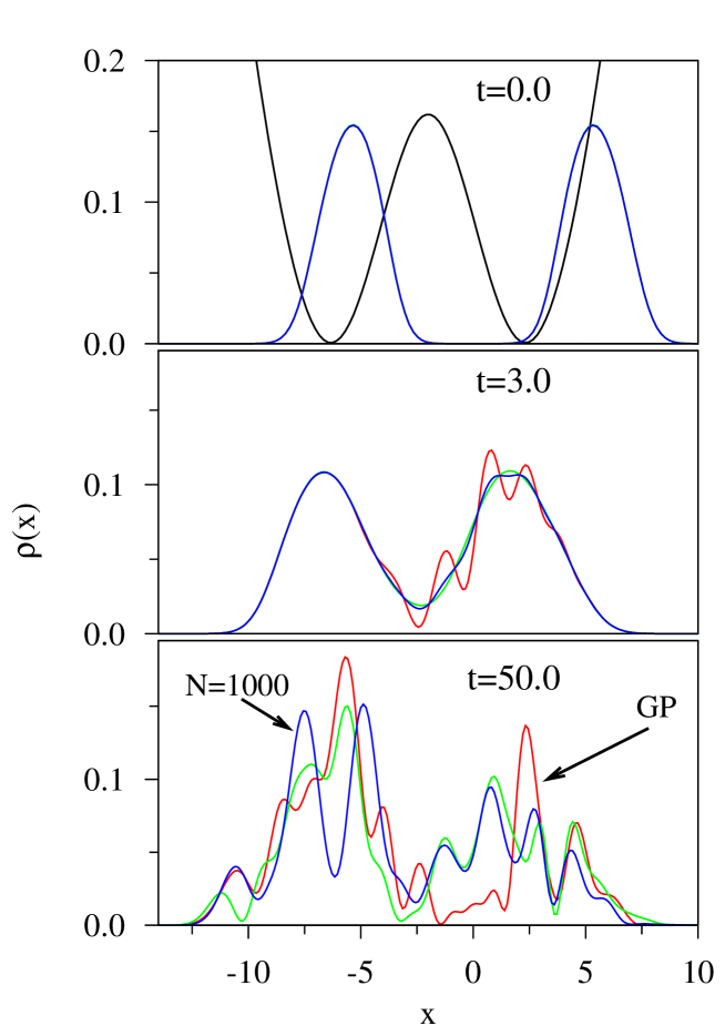
Figure 1: (Color online) Many-body time evolution of two condensates made of $N=100$ (in green) and $N=1000$ (in blue) bosons in a double-well potential with corresponding interaction strengths $\lambda_{0}=\frac{9.99}{N-1}$ computed by the MCTDHB(2) theory. For comparison, the corresponding solution computed by the time-dependent Gross-Pitaevskii equation is also displayed (in red). Shown are three time snapshots of the density $\rho(x,t)$, normalized to 1. At $t=0$ all densities are identical on the scale show. To guide the eye, the double-well trap potential in which the condensates evolve is also illustrated (in black). The quantities shown are dimensionless. See text for more details.

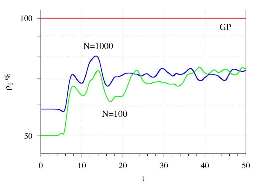
Figure 2: (Color online) Natural occupation numbers of two condensates made of $N=100$ (in green) and $N=1000$ (in blue) bosons in a double-well potential (same parameters as in Fig. 1). Shown in percents is the largest occupation $\rho_{1}$ ($\rho_{2}=100\%-\rho_{1}$; $\rho_{2}$ is not shown). As time passes, the natural occupation numbers change substantially. For comparison, the corresponding fixed $100\%$ occupation of the time-dependent Gross-Pitaevskii theory is also displayed (in red). The quantities shown are dimensionless. See text for more details.

We compare the time-dependent dynamics of the mean-field Gross-Pitaevskii and of the many-body MCTDHB(2) approach. Since visualization of the time-dependent many-body wavefunction $\Psi(t)$ is quite cumbersome, we plot in Fig. 1 snapshot of the density, $\rho(x,t)=\sum^{2}_{k,q=1}\rho_{kq}(t)\phi^{\ast}_{k}(x,t)\phi_{q}(x,t)$, at different times and compare with the respective Gross-Pitaevskii theory. Furthermore, in Fig. 2 we display the natural occupation numbers $\rho_{j}(t),\,j\!=\!1,2$ of $\Psi(t)$, i.e., the eigenvalues of the corresponding reduced one-particle density, $\rho(x|x^{\prime};t)=\sum^{2}_{j=1}\rho_{j}(t)\phi^{\ast{NO}}_{j}(x^{\prime},t)\phi^{NO}_{j}(x,t)$, at each point in time. Of course, in Gross-Pitaevskii theory there is only one occupation number, $\rho_{1}=100\%$.

Let us analyze the densities shown in Fig. 1. Since the barrier between the two potential wells is initially quite high, the corresponding three densities coincide at $t=0$, see top panel of Fig. 1. At $t=3.0$ we already see an observable difference. The Gross-Pitaevskii density acquires wiggles due to collisions with the potential walls. On the other hand, the densities in the many-body calculations show almost no wiggles for $N=100$ and $N=1000$ bosons. By $t=50.0$ all three densities have substantially distorted from the initial conditions and exhibit multiple density wiggles of various sizes and depths. All densities are different from one another. In particular, the systems with $N=100$ and $N=1000$ bosons which, as we have mentioned above, have the same time evolution on the mean-field level are actually showing quite distinct evolutions on the many-body level, see Fig. 1.

Next, let us analyze the natural occupation numbers of $\Psi(t)$. In the Gross-Pitaevskii dynamics the initial condition, which is the ground state of the potential $V_{0}(x)$ computed by imaginary-time propagation of the Gross-Pitaevskii equation, is fully coherent and hence there is only one occupation number, $\rho_{1}=100\%$. This property of the condensate obviously does not change in time when the time-dependent Gross-Pitaevskii equation governs the dynamics. Contrastly, on the many-body level the situation differs substantially. First, the initial conditions for $N=100$ and $N=1000$ bosons, which are the respective ground states of the potential $V_{0}(x)$ computed by imaginary-time propagation of the MCTDHB(2) equations, actually correspond to fragmented condensates, see Fig. 2 at $t=0$. Most importantly, in the course of the many-body time evolution of the bosonic systems the natural-orbital occupations change in time by at least $20\%$. This suggests an intricate and important property of the many-body dynamics which by definition cannot be accessed by the mean-field dynamics.

All in one, the numerical results of the application of MCTDHB(2) to simple trapped bosonic systems demonstrate that the many-boson dynamics in traps is manageable and intriguing, and that it can also be quite different from the mean-field dynamics.

V Summary and conclusions

The evolution of Bose-Einstein condensates has been extensively studied by the well-known time-dependent Gross-Pitaevskii equation which assumes all bosons to reside in the same time-dependent orbital and hence the condensate to be coherent at all times. In this work we address the evolution of condensates on the many-body level, and develop and report on an essentially-exact and numerically-efficient approach for the solution of the time-dependent many-boson Schrödinger equation. We term our approach multi-configurational time-dependent Hartree for bosons (MCTDHB).

In the MCTDHB, the ansatz for the many-boson wavefunction is taken as a linear combination of all possible time-dependent permanents made by distributing $N$ bosons over $M$ orthogonal time-dependent orbitals. The evolution of the many-body wavefunction is then determined by utilizing a standard time-dependent variational principle – either the Lagrangian formulation or the Dirac-Frenkel variational principle. Performing the variation, we arrive at two sets of coupled equations-of-motion, one for the orbitals and one for the expansion coefficients. The first set comprises of first-order differential equations in time and non-linear integro-differential equations in position space. The second set consists of first-order differential equations with time-dependent coefficients. MCTDHB naturally relates – by performing propagation in imaginary time – to the recently developed and successfully employed general variational mean-body theory with complete self-consistency for stationary many-boson systems (MCHB). From another instructive perspective, MCTDHB can be seen as specification of the successful multi-dimensional wavepacket-propagation approach MCTDH to systems of identical bosons. By explicitly exploiting bosons’ statistics and the fact that only a two-body interaction is needed it is now possible to successfully and quantitatively attack the dynamics of a much larger number of bosons with the developed MCTDHB theory.

With an essentially-exact and full many-body theory for the dynamics of bosonic systems, we can now investigate the many-body correlation effects coming atop the time-dependent Gross-Pitaevskii GPO1 ; GPO2 and multi-orbital OAL_PLA_2007 mean-field dynamics of unfragmented and fragmented Bose-Einstein condensates, respectively. Another promising direction would be to utilize MCTDHB for devising and investigating strategies for approximate many-body time-dependent approaches such as Hilbert-space truncation schemes.

Finally, illustrative numerical examples of the many-body evolution of condensates in a one-dimensional double-well trap are provided, demonstrating an intricate dynamics of the density and natural orbitals as time progresses which are not accounted for by the respective Gross-Pitaevskii mean-field dynamics. This is the tip of the iceberg of many-body dynamical properties of Bose-Einstein condensates and interacting bosons which await many more investigations with MCTDHB.

Appendix A Matrix elements of two-body operators and of the two-body density matrix

Matrix elements of the two-body operator $\hat{W}$ between two general permanents $\left|\vec{n};t\right>$ and $\left|\vec{n}^{\prime};t\right>$. The permanent denoted by $\left|\vec{n}_{q}^{k};t\right>$ differs from $\left|\vec{n};t\right>$ by an excitation of one boson from the $q$-th to the $k$-th orbital, whereas $\left|\vec{n}_{ql}^{ks};t\right>$ differs from $\left|\vec{n};t\right>$ by excitations of two bosons, one boson from the $q$-th to the $k$-th orbital and a second boson from the $l$-th to the $s$-th orbital:

$$\left<\vec{n};t\left|\hat{W}\right|\vec{n};t\right>=\frac{1}{2}\sum_{j=1}^{M}n_{j}\left[\left(n_{j}-1\right)W_{jjjj}+\sum_{\{i\neq j\}=1}^{M}n_{i}W_{ji[ji]}\right],$$

$$\left<\vec{n}_{q}^{k};t\left|\hat{W}\right|\vec{n};t\right>=\sqrt{(n_{k}+1)n_{q}}\left[n_{k}W_{kkkq}+(n_{q}-1)W_{kqqq}+\sum_{\{i\neq q,k\}=1}^{M}n_{i}W_{ki[iq]}\right]$$

$$\left<\vec{n}_{qq}^{kk};t\left|\hat{W}\right|\vec{n};t\right>=\frac{1}{2}\sqrt{(n_{k}+1)(n_{k}+2)(n_{q}-1)n_{q}}W_{kkqq}$$

$$\left<\vec{n}_{ql}^{kk};t\left|\hat{W}\right|\vec{n};t\right>=\sqrt{(n_{k}+1)(n_{k}+2)n_{q}n_{l}}W_{kkql}$$

$$\left<\vec{n}_{qq}^{ks};t\left|\hat{W}\right|\vec{n};t\right>=\sqrt{(n_{k}+1)(n_{s}+1)(n_{q}-1)n_{q}}W_{ksqq}$$

$$\left<\vec{n}_{ql}^{ks};t\left|\hat{W}\right|\vec{n};t\right>=\sqrt{(n_{k}+1)(n_{s}+1)n_{q}n_{l}}W_{ks[ql]}.$$ (37)

Different indices $k,s,q,l$ cannot have the same value. All other matrix elements vanish.

Matrix elements of the reduced two-body density $\rho({\bf r}_{1},{\bf r}_{2}|{\bf r}^{\prime}_{1},{\bf r}^{\prime}_{2};t)=\left<\Psi(t)\left|\hat{\mathbf{\Psi}}^{\dagger}({\bf r}^{\prime}_{1})\hat{\mathbf{\Psi}}^{\dagger}({\bf r}^{\prime}_{2})\hat{\mathbf{\Psi}}({\bf r}_{1})\hat{\mathbf{\Psi}}({\bf r}_{2})\right|\Psi(t)\right>$ of the many-boson state $\left|\Psi(t)\right>=\sum_{\vec{n}}C_{\vec{n}}(t)\left|\vec{n};t\right>$:

$$\rho_{kkkk}=\sum_{\vec{n}}C_{\vec{n}}^{\ast}C_{\vec{n}}\left(n^{2}_{k}-n_{k}\right),$$

$$\rho_{ksks}=\sum_{\vec{n}}C_{\vec{n}}^{\ast}C_{\vec{n}}n_{k}n_{s},$$

$$\rho_{kkqq}=\sum_{\vec{n}}C_{\vec{n}}^{\ast}C_{\vec{n}_{kk}^{qq}}\sqrt{(n_{k}-1)n_{k}(n_{q}+1)(n_{q}+2)},$$

$$\rho_{kkkl}=\sum_{\vec{n}}C_{\vec{n}}^{\ast}C_{\vec{n}_{k}^{l}}(n_{k}-1)\sqrt{n_{k}(n_{l}+1)},$$

$$\rho_{ksss}=\sum_{\vec{n}}C_{\vec{n}}^{\ast}C_{\vec{n}_{k}^{s}}n_{s}\sqrt{n_{k}(n_{s}+1)},$$

$$\rho_{kkql}=\sum_{\vec{n}}C_{\vec{n}}^{\ast}C_{\vec{n}_{kk}^{ql}}\sqrt{(n_{k}-1)n_{k}(n_{q}+1)(n_{l}+1)},$$

$$\rho_{ksqq}=\sum_{\vec{n}}C_{\vec{n}}^{\ast}C_{\vec{n}_{ks}^{qq}}\sqrt{n_{k}n_{s}(n_{q}+1)(n_{q}+2)},$$

$$\rho_{kssl}=\sum_{\vec{n}}C_{\vec{n}}^{\ast}C_{\vec{n}_{k}^{l}}n_{s}\sqrt{n_{k}(n_{l}+1)},$$

$$\rho_{ksql}=\sum_{\vec{n}}C_{\vec{n}}^{\ast}C_{\vec{n}_{ks}^{ql}}\sqrt{n_{k}n_{s}(n_{q}+1)(n_{l}+1)}.\$$ (38)

Different indices $k,s,q,l$ cannot have the same value. All other matrix elements can be computed due to the symmetries of the two-body operator, $\rho_{ksql}=\rho_{kslq}=\rho_{sklq}=\rho_{skql}$, and its hermiticity, $\rho^{\ast}_{ksql}=\rho_{qlks}$.

Appendix B Derivation of the MCTDHB equations-of-motion starting from the Dirac-Frenkel variational principle

The Dirac-Frenekl variational principle reads DF1 ; DF2 :

$$\left<\delta\Psi(t)\left|\hat{H}-i\frac{\partial}{\partial t}\right|\Psi(t)\right>=0.$$ (39)

Given the MCTDHB ansatz for the many-boson wavefunction, $\left|\Psi(t)\right>=\sum_{\vec{n}}C_{\vec{n}}(t)\left|\vec{n};t\right>$, the variation $\delta\Psi(t)$ in Eq. (39) is performed separately with respect to the expansion coefficients $\{C_{\vec{n}}(t)\}$ and with respect to the orbitals $\{\phi_{k}({\bf r},t)\}$.

We begin as in the main text with the coefficients. From the structure of $\left|\Psi(t)\right>$ as a sum of permanents one obviously has

$$\frac{\partial\left<\Psi(t)\right|}{\partial C^{\ast}_{\vec{n}}(t)}=\left<\vec{n};t\right|.$$ (40)

Hence, making use of the orthonormality relation of the permanents $\left<\vec{n};t\left|\right.\vec{n}^{\prime};t\right>=\delta_{\vec{n},\vec{n}^{\prime}}$ one straightforwardly finds:

$$\left(\frac{\partial}{\partial C^{\ast}_{\vec{n}}(t)}\left<\Psi(t)\left|\left)\hat{H}-i\frac{\partial}{\partial t}\right|\Psi(t)\right>\right.\right.=0\ \ \Longrightarrow\mbox{\boldmath$\mathcal{H}$}(t){\bf C}(t)=i\frac{\partial{\bf C}(t)}{\partial t},$$ (41)

which is precisely the result depicted in Eq. (10).

To proceed for the orbitals, we need a few identities and relations. Starting from the basic definitions $\hat{\mathbf{\Psi}}({\bf r})=\sum_{k}b_{k}(t)\phi_{k}({\bf r},t)$ and $b_{k}(t)=\int\phi_{k}^{\ast}({\bf r},t)\hat{\mathbf{\Psi}}({\bf r})d{\bf r}$ connecting the annihilation and field operators one readily has,

$$\frac{\delta b_{k}(t)}{\delta\phi_{q}^{\ast}({\bf r},t)}=\delta_{kq}\hat{\mathbf{\Psi}}({\bf r}).$$ (42)

With the help of (42) we can take the variation of a single permanent $\left<\vec{n};t\right|$,

$$\frac{\delta\left<\vec{n};t\right|}{\delta\phi_{k}^{\ast}({\bf r},t)}=\left<\vec{n};t\right|b_{k}^{\dagger}(t)\hat{\mathbf{\Psi}}({\bf r}),$$ (43)

and from it of the ’bra’ $\left<\Psi(t)\right|$ itself,

$$\frac{\delta\left<\Psi(t)\right|}{\delta\phi_{k}^{\ast}({\bf r},t)}=\left<\Psi(t)\right|b_{k}^{\dagger}(t)\sum_{q}b_{q}(t)\phi_{q}({\bf r},t).$$ (44)

On the ’ket’ side of Eq. (39) we keep in mind that,

$$i\frac{\partial}{\partial t}\left|\Psi(t)\right>=\sum_{\vec{n}}\left\{i\frac{\partial C_{\vec{n}}(t)}{\partial t}+C_{\vec{n}}(t)i\frac{\partial}{\partial t}\right\}\left|\vec{n};t\right>.$$ (45)

Utilizing Eqs. (41), (44) and (45) and the usual commutation relations between the bosonic annihilation and creation operators, we evaluate separately the contributions coming from the one-body $\hat{h}-i\frac{\partial}{\partial t}$ and two-body $\hat{W}$ operators. Combining the results one finds:

$$\left(\frac{\delta}{\delta\phi^{\ast}_{k}({\bf r},t)}\left<\Psi(t)\left|\left)\hat{H}-i\frac{\partial}{\partial t}\right|\Psi(t)\right>\right.\right.=0\ \ \Longrightarrow$$

$$\sum^{M}_{q=1}\left\{\rho_{kq}\left(\hat{h}-i\frac{\partial}{\partial t}\right)+\sum^{M}_{s,l=1}\rho_{ksql}\hat{W}_{sl}\right\}\left|\phi_{q}\right>=-\sum^{M}_{j=1}\left<\Psi\left|b_{k}^{\dagger}\left[\hat{H}-i\frac{\partial}{\partial t},b_{j}\right]\right|\Psi\right>\left|\phi_{j}\right>.\$$ (46)

To show that (B) is exactly Eq. (22) we evaluate the commutator on the right-hand-side of the former,

$$\left[\hat{H}-i\frac{\partial}{\partial t},b_{j}\right]=-\sum_{q}\left\{\left(h_{jq}-\left(i\frac{\partial}{\partial t}\right)_{jq}\right)b_{q}+\sum_{s,l}W_{jsql}b_{s}^{\dagger}b_{q}b_{l}\right\},$$ (47)

from which we readily get that the right-hand-side of (B) is nothing but (sum over) $\mu_{kj}(t)$ of Eq. (22), i.e., that

$$\mu_{kj}(t)=-\left<\Psi\left|b_{k}^{\dagger}\left[\hat{H}-i\frac{\partial}{\partial t},b_{j}\right]\right|\Psi\right>.$$ (48)

From this point on the two derivations coincide, leading as expected to identical equations-of-motion of MCTDHB.

We conclude the appendix by pointing out an additional connection between the two variational formulations used in this work to derive the MCTDHB equations-of-motion. Eqs. (B), (47) and (48) hint towards another role played by the Lagrange multipliers $\mu_{kj}(t)$ employed in the main text. Since in the Dirac-Frenkel formulation the variation is taken before matrix elements are computed, whereas in the Lagrangian formulation the situation reverses, there would have been ’missing’ terms in the equations-of-motion derived by the Lagrangian formulation. The introduction of the Lagrange multipliers in Eq. (6) exactly ’compensates’ for these terms.

References

- (1) M. H. Anderson, J. R. Ensher, M. R. Matthews, C. E. Wieman, and E. A. Cornell, Science 269, 198 (1995).
- (2) K. B. Davis, M.-O. Mewes, M. R. Andrews, N. J. van Druten, D. S. Durfee, D. M. Kurn, and W. Ketterle, Phys. Rev. Lett. 75, 3969 (1995).
- (3) W. Ketterle, Rev. Mod. Phys. 74, 1131 (2002).
- (4) E. A. Cornell and C. E. Wieman, Rev. Mod. Phys. 74, 875 (2002).
- (5) J. I. Cirac and P. Zoller, Phys. Rev. Lett. 74, 4091 (1995).
- (6) G. K. Brennen, C. M. Caves, P. S. Jessen, and I. H. Deutsch, Phys. Rev. Lett. 82, 1060 (1999).
- (7) C. Orzel, A. K. Tuchman, M. L. Fenselau, M. Yasuda, M. A. Kasevich, Science 291, 2386 (2001).
- (8) A. J. Leggett, Rev. Mod. Phys. 73, 307 (2001).
- (9) C. J. Pethick and H. Smith, Bose-Einstein Condensation in Dilute Gases (Cambridge University Press, Cambridge, 2002).
- (10) L. Pitaevskii and S. Stringari, Bose-Einstein Condensation (Oxford University Press, Oxford, 2003).
- (11) E. P. Gross, Nuovo Cimento 20, 454 (1961).
- (12) L. P. Pitaevskii, Zh. Eksp. Teor. Fiz. 40, 646 (1961) [Sov. Phys. JETP 13, 451 (1961)].
- (13) L. D. Carr, Charles W. Clark, and W. P. Reinhardt, Phys. Rev. A 62, 063610 (2000).
- (14) R. Baer, Phys. Rev. A 62, 063810 (2000).
- (15) H. Saito and M. Ueda, Phys. Rev. Lett. 90, 040403 (2003).
- (16) Z. X. Liang, Z. D. Zhang, and W. M. Liu, Phys. Rev. Lett. 94, 050402 (2005).
- (17) S. Komineas and J. Brand, Phys. Rev. Lett. 95, 110401 (2005).
- (18) L. Sanchez-Palencia and L. Santos, Phys. Rev. A 72, 053607 (2005).
- (19) D. Ananikian and T. Bergeman, Phys. Rev. A, 73, 013604 (2006).
- (20) T.-L. Ho and V. B. Shenoy, Phys. Rev. Lett. 77, 3276 (1996).
- (21) B. D. Esry, C. H. Greene, J. P. Burke, Jr., and J. L. Bohn, Phys. Rev. Lett. 78, 3594 (1997).
- (22) H. Pu and N. P. Bigelow, Phys. Rev. Lett. 80, 1130 (1998).
- (23) H. Pu and N. P. Bigelow, Phys. Rev. Lett. 80, 1134 (1998).
- (24) E. Timmermans, Phys. Rev. Lett. 81, 5718 (1998).
- (25) P. Öhberg and L. Santos, Phys. Rev. Lett. 86, 2918 (2001).
- (26) L. S. Cederbaum and A. I. Streltsov, Phys. Lett. A 318, 564 (2003).
- (27) O. E. Alon, A. I. Streltsov, and L. S. Cederbaum, Phys. Lett. A 362, 453 (2007).
- (28) A. I. Streltsov and L. S. Cederbaum, Phys. Rev. A 71, 063612 (2005).
- (29) O. E. Alon, A. I. Streltsov, and L. S. Cederbaum, Phys. Rev. Lett 95, 030405 (2005).
- (30) O. E. Alon and L. S. Cederbaum, Phys. Rev. Lett 95, 140402 (2005).
- (31) O. E. Alon, A. I. Streltsov, and L. S. Cederbaum, Phys. Rev. Lett 97, 230403 (2006).
- (32) L. S. Cederbaum, A. I. Streltsov, Y. B. Band, O. E. Alon, Phys. Rev. Lett., in press (cond-mat/0701277).
- (33) A. Minguzzi, S. Succi, F. Toschi, M. P. Tosi and P. Vignolo, Phys. Rep. 395, 223 (2004).
- (34) C.-S. Chuu, F. Schreck, T. P. Meyrath, J. L. Hanssen, G. N. Price, and M. G. Raizen, Phys. Rev. Lett. 95, 260403 (2005).
- (35) M. Albiez, R. Gati, J. Fölling, S. Hunsmann, M. Cristiani, and M. K. Oberthaler, Phys. Rev. Lett. 95, 010402 (2005).
- (36) A. I. Streltsov, O. E. Alon, and L. S. Cederbaum, Phys. Rev. A 73, 063626 (2006).
- (37) A. I. Streltsov, O. E. Alon, and L. S. Cederbaum, cond-mat/0612616.
- (38) C. Menotti, J. R. Anglin, J. I. Cirac, and P. Zoller, Phys. Rev. A 63, 023601 (2001).
- (39) D. Masiello and W. P. Reinhardt, cond-mat/0702067.
- (40) N. Makri and W. H. Miller, J. Chem. Phys. 87, 5781 (1987).
- (41) R. Kosloff, A. D. Hammerich, and M. A. Ratner, in: J. Jortner, B. Pullman (Eds.), Large Finite Systems: Proceedings of the Twentieth Jerusalem Symposium of Quantum Chemistry and Biochemistry (Reidel, Dordrecht, 1987).
- (42) A. D. Hammerich, R. Kosloff and M. A. Ratner, Chem. Phys. Lett. 171, 97 (1990).
- (43) H.-D. Meyer, U. Manthe, and L. S. Cederbaum, Chem. Phys. Lett. 165, 73 (1990).
- (44) U. Manthe, H.-D. Meyer, and L. S. Cederbaum, J. Chem. Phys. 97, 3199 (1992).
- (45) M. H. Beck and H.-D. Meyer, Z. Phys. D 42, 113 (1997).
- (46) M. H. Beck, A. Jäckle, G. A. Worth and H.-D. Meyer, Phys. Rep. 324, 1 (2000).
- (47) S. Zöllner, H.-D. Meyer, and P. Schmelcher, Phys. Rev. A 74, 053612 (2006).
- (48) S. Zöllner, H.-D. Meyer, and P. Schmelcher, Phys. Rev. A 74, 063611 (2006).
- (49) J. Zanghellini, M. Kitzler, C. Fabian, T. Brabec, and A. Scrinzi, Laser Phys. 13, 1064 (2003).
- (50) T. Kato and H. Kono, Chem. Phys. Lett. 392, 533 (2004).
- (51) M. Nest, T. Klamroth, and P. Saalfrank, J. Chem. Phys. 122, 124102 (2005).
- (52) M. D. Girardeau and E. M. Wright, Phys. Rev. Lett. 84, 5239 (2000).
- (53) P. Kramer and M. Saracento, Geometry of the time-dependent variational principle (Springer, Berlin, 1981).
- (54) H.-J. Kull and D. Pfirsch, Phys. Rev. E 61, 5940 (2000).
- (55) P. A. M. Dirac, Proc. Cambridge Phil. Soc. 26, 376 (1930).
- (56) J. Frenkel, Wave Mechanics (Oxford Univ. Press, Oxford, 1934).
- (57) H.-D. Meyer and G. A. Worth, Theor. Chem. Acc. 109 251 (2003).
- (58) T. Jun Park and J. C. Light, J. Chem. Phys. 85, 5870 (1986).
- (59) W. H. Press, S. A. Teukolsky, W. T. Vetterling, and B. P. Flannery, Numerical Recipes in Fortran (Cambridge Univ. Press, Cambridge, 1992), 2nd ed.
- (60) Z. Bačić and J. C. Light, J. Chem. Phys. 85, 4594 (1986).