Autocorrelation functions in phase-ordering kinetics from local scale-invariance

Abstract

The explicit calculation of the scaling form of the two-time autocorrelation function in phase-ordering kinetics and in those cases of non-equilibrium critical dynamics where the dynamical exponent $z=2$ through the extension of dynamical scaling to local scale-invariance is reviewed. Conceptually, this mainly requires an extension from the usually considered $d$-dimensional ageing or Schrödinger algebras to a new kind of representation of the conformal algebra in $d+2$ dimensions. Explicit tests in several exactly solved models of simple magnets and through simulations in the $2D$ Ising and $q$-states Potts models ($q=2,3,8$) quenched to $T<T_{c}$ are presented and the extension to systems with non-equilibrium steady-states is discussed through two exactly solvable models as well. In the context of surface growth models, possible generalizations for a dynamical exponent $z=4$ and beyond are discussed.

1 Introduction

Phase-ordering kinetics [17] may occur if a magnet is rapidly brought (‘quenched’) from some initial disordered state to some temperature $T<T_{c}$ below its critical temperature $T_{c}>0$. At equilibrium, such systems have at least two equivalent macroscopically ordered thermodynamic states. Because of the competition between these two equilibrium states, the system cannot simply relax within a finite time towards one of them but rather, stimulated by the small effective magnetic fields which are created by the environment of each magnetic atom, ordered domains will form and subsequently grow. Although the average magnetization, if initially zero, will not change, there is a slow, non-exponential relaxation as the walls separating the ordered domains slowly move. For a spatially infinite system, this gradual coarsening process will continue indefinitely, and the state of the system and the behaviour of time-dependent observables will depend on the age of the system, that is the time elapsed since the quench. In addition, as will be discussed in detail in this article, dynamical scaling is observed, although neither of the equilibrium states by itself is scale-invariant. The three properties (i) slow, non-exponential dynamics, (ii) breaking of time-translation invariance and (iii) some kind of dynamical scaling are the constitutive properties of ageing systems.

Physical ageing was first identified in celebrated experiments on the mechanical response of certain glassy systems to external stress [97]. For a better theoretical understanding, the quite recent realization that very similar phenomena can also be found in simple magnets, without disorder nor frustrations, might lead to conceptual insights which in turn could become also fruitful in more complex systems. For recent reviews of this intensively studied topic, see [31, 46, 30, 21, 28, 41, 56, 61, 62].

To begin, we recall some facts about dynamical scaling of phase-ordering systems. Unless explicitly stated otherwise, we assume that throughout the order-parameter is non-conserved by the dynamics and that the initial state is totally disordered. For late time, linear size $L$ of the ordered domains grows as $L\sim t^{1/z}$ and it is known that the dynamical exponent $z=2$ for a non-conserved order-parameter [18]. If $\phi(t,\boldsymbol{r})$ is the order-parameter at time $t$ and location $\boldsymbol{r}$ the following dynamical scaling of the two-time autocorrelation $C$ and (linear) autoresponse function $R$ is usually assumed

$$C(t,s) = \langle\phi(t,\boldsymbol{r})\phi(s,\boldsymbol{r})\rangle~{}~{}\sim s^{-b}f_{C}(t/s)$$ (1)

$$R(t,s) = \left.\frac{\delta\langle\phi(t,\boldsymbol{r})\rangle}{\delta h(s,\boldsymbol{r})}\right|_{h=0}\sim s^{-1-a}f_{R}(t/s)$$ (2)

where $h(s,\boldsymbol{r})$ is the conjugate magnetic field at time $s$ and location $\boldsymbol{r}$. The scaling behaviour is expected to apply in the so-called ageing regime where

$$t,s\gg t_{\rm micro}\mbox{\rm~{}~{}and~{}~{}}t-s\gg t_{\rm micro}$$ (3)

where $t_{\rm micro}$ is a microscopic time-scale [104]. In writing eqs. (1,2) it was tacitly assumed that the scaling derives from the algebraic time-dependence of the single characteristic length-scale $L=L(t)\sim t^{1/z}$ which measures the linear size of correlated or ordered clusters and where $z$ is the dynamic exponent. Under these assumptions, the above forms define the non-equilibrium exponents $a$ and $b$ and the scaling functions $f_{C}(y)$ and $f_{R}(y)$. For large arguments $y=t/s\to\infty$, one generically expects

$$f_{C}(y)\sim y^{-\lambda_{C}/z}\;\;,\;\;f_{R}(y)\sim y^{-\lambda_{R}/z}$$ (4)

where $\lambda_{C}$ and $\lambda_{R}$, respectively, are known as autocorrelation [39, 66] and autoresponse exponents [86]. In non-disordered magnets with short-ranged initial conditions one usually has $\lambda_{C}=\lambda_{R}$, but this is need no longer be true if either of these conditions is relaxed [81, 86, 94, 58]. Field-theoretical considerations for systems quenched to $T=T_{c}$ show that for a non-conserved order-parameter the calculation of $\lambda_{C,R}$ requires an independent renormalization and hence one cannot expect to find a scaling relation between these and equilibrium exponents (including $z$) [68]. For phase-ordering (quenches to $T<T_{c}$) a well-known result due to Bray [17] relates the difference $\lambda_{C}-\lambda_{R}$ to an exponent describing the fall-off of the initial correlator. In particular it can be shown that $\lambda_{C}=\lambda_{R}$ for short-ranged initial correlations [17]. This same result can alternatively be derived from local scale-invariance [87] (see section 3).

The values of the exponents $a$ and $b$ are as follows for phase-ordering. First, one usually observes simple scaling of $C(t,s)=f_{C}(t/s)$, hence $b=0$. Second, the value of $a$ depends on whether the equilibrium correlator decays exponentially (‘short-ranged’) or algebraically (‘long-ranged’). This defines the classes S and L, respectively and one has [13, 26, 51, 54]

$$C_{\rm eq}(\boldsymbol{r})\sim\left\{\begin{array}[]{l}e^{-|\boldsymbol{r}|/\xi}\\ |\boldsymbol{r}|^{-(d-2+\eta)}\end{array}\right.\;\;\Longrightarrow\;\;\left\{\begin{array}[]{l}\mbox{\rm class S}\\ \mbox{\rm class L}\end{array}\right.\;\;\Longrightarrow\;\;a=\left\{\begin{array}[]{c}1/z\\ (d-2+\eta)/z\end{array}\right.$$ (5)

Examples for short-ranged models (class S) include the Ising or Potts models in $d>1$ dimensions, while the spherical model or the $2D$ XY model below the Kosterlitz-Thouless transition are examples for long-ranged systems (class L).

A much harder problem is posed by the quest to find the universal scaling functions $f_{R}(y)$ and $f_{C}(y)$. Indeed, one might consider the analogy with equilibrium critical phenomena where simple scale-invariance can be extended to conformal invariance, under quite general conditions. Since conformal transformations are scale-transformations with a spatially varying rescaling factor (such that angles are conserved), one can inquire about the possibility to similarly extend dynamical scaling to an invariance of the physical system under more general, local scale-transformations [49, 50]. Specifically, motivated by the analogy with conformal invariance [88, 12], the transformations of time

$$t\mapsto t^{\prime}=\frac{\alpha t+\beta}{\gamma t+\delta}\;\;;\;\;\alpha\delta-\beta\gamma=1$$ (6)

were considered to which transformations of space $\boldsymbol{r}\mapsto\boldsymbol{r}^{\prime}$ must be added in such a way that,say, these local scale-transformation form a Lie algebra. Furthermore, it can be argued that the linear response functions should transform covariantly under such local scale-transformations (at least if the scaling operators from which they are built are so-called quasi-primary operators) [49, 50, 87]. Taking into account that time-translations cannot be part of local scale-transformations as applied to ageing phenomena (hence $\beta=0$ in (6)), this leads to [87, 57, 52] ($\Theta$ is the Heaviside function)

$$f_{R}(y)=f_{0}\,y^{1+a^{\prime}-\lambda_{R}/z}(y-1)^{-1-a^{\prime}}\Theta(y-1)$$ (7)

such that the form of $f_{R}(y)$ is determined by the two exponents $\lambda_{R}/z$ and $a^{\prime}$ which are related to the scaling dimensions of the order-parameter $\phi$ and the associate response field $\widetilde{\phi}$ and $f_{0}$ is a normalization constant. By now there exists quite a long list of models where either the exact solution or numerical data for $R(t,s)=\langle\phi(t)\widetilde{\phi}(s)\rangle$ are compatible with the prediction (7) of local scale-invariance as reviewed in detail in [61, 62].

Here, we shall address the question how to find $f_{C}(y)$ from an extension of dynamical scaling to local scale-invariance. Although the method has been successfully applied in various contexts, see [55, 6, 76, 67, 57, 90, 9], only the barest outline of it was ever published [55, 57]. As we shall see, the analytical calculation of correlators is quite a demanding task, be it in the context of closed-form approximations [16, 100, 91], perturbative schemes [74, 78, 79] or else from a dynamical symmetry. Since $z=2$ in phase-ordering kinetics, a natural candidate for a local scale-symmetry is provided by the well-known Schrödinger group and/or some of its subgroups. We shall recall their definition in section 2 and remind that the Schrödinger group is a group of dynamical symmetries of the free diffusion equation. It may be less well-known that, provided one considers the diffusion constant as an additional variable, there is a larger dynamical symmetry isomorphic to a conformal group in $d+2$ dimensions [20, 52]. These results may be extended to slightly more general diffusion equations. Next, we consider the Langevin description for phase-ordering kinetics where there exists an exact reduction formula which reduces the calculation of any $n$-point correlation/response function to the calculation of certain correlators/responses in the noiseless part of the theory only, given that so-called Bargman superselection rules for that deterministic part are valid. In section 3, we recall first the standard result from Schrödinger-invariance for the required three-point function and then show how using the previously discussed extension to a conformal group the two-time correlation function can be found. In section 4 we review existing tests of this prediction, both analytical and numerical. Finally, in section 5 we present a short outlook how the methods reviewed here might be extendable to cases where $z\neq 2$ and conclude in section 6. A technical point on the determination of the autocorrelation function is treated in the appendix.

2 Dynamical symmetries: Schrödinger, ageing and conformal

In this section, we recall those elements of local scale-invariance, specialized to the case $z=2$, which we shall need for the explicit calculation of two-time correlations.

2.1 Schrödinger-invariance of the free diffusion equation

Consider the dynamical symmetries of the free diffusion (or free Schrödinger) equation

$$2{\cal M}\partial_{t}\phi=\Delta\phi$$ (8)

where $\Delta=\boldsymbol{\nabla}\cdot\boldsymbol{\nabla}$ is the spatial laplacian and the ‘mass’ $\cal M$ plays the rôle of a kinetic coefficient. The Schrödinger-group Sch($d$) (actually, already found by Lie more than a century ago) contains the space-time transformations

$$t\mapsto t^{\prime}=\frac{\alpha t+\beta}{\gamma t+\delta}\;\;;\;\;\boldsymbol{r}\mapsto\boldsymbol{r}^{\prime}=\frac{{\cal R}\boldsymbol{r}+\boldsymbol{v}t+\boldsymbol{a}}{\gamma t+\delta}\;\;,\;\;\alpha\delta-\beta\gamma=1$$ (9)

where $\alpha,\beta,\gamma,\delta,\boldsymbol{v},\boldsymbol{a}$ are real (vector) parameters and ${\cal R}$ is a rotation matrix in $d$ spatial dimensions. The group acts projectively on a solution $\phi$ of the diffusion equation through $(t,\boldsymbol{r})\mapsto g(t,\boldsymbol{r})$, $\phi\mapsto T_{g}\phi$

$$\left(T_{g}\phi\right)(t,\boldsymbol{r})=f_{g}(g^{-1}(t,\boldsymbol{r}))\,\phi(g^{-1}(t,\boldsymbol{r}))$$ (10)

where $g$ is an element of the Schrödinger group and the companion function reads [82, 85]

$$f_{g}(t,\boldsymbol{r})=(\gamma t+\delta)^{-d/2}\exp\left[-\frac{{\cal M}}{2}\frac{\gamma\boldsymbol{r}^{2}+2{\cal R}\boldsymbol{r}\cdot(\gamma\boldsymbol{a}-\delta\boldsymbol{v})+\gamma\boldsymbol{a}^{2}-t\delta\boldsymbol{v}^{2}+2\gamma\boldsymbol{a}\cdot\boldsymbol{v}}{\gamma t+\delta}\right]$$ (11)

It is then natural to include also arbitrary phase-shifts of the wave function $\phi$ within the Schrödinger group Sch($d$). We shall denote the Lie algebra of Sch($d$) by $\mathfrak{sch}_{d}$. The invariance of the space of solutions of the free diffusion equation (8) under this group can be illustrated in $d=1$ by introducing the Schrödinger operator

$${\cal S}:=2M_{0}Y_{-1}-Y_{-1/2}^{2}=2{\cal M}\partial_{t}-\partial_{r}^{2}$$ (12)

In what follows, we shall restrict calculations to the case $d=1$ since the extensions to
$d>1$ will be obvious. The Schrödinger Lie algebra $\mathfrak{sch}_{1}=\langle X_{-1,0,1},Y_{-\frac{1}{2},\frac{1}{2}},M_{0}\rangle$ is spanned by the infinitesimal generators of temporal and spatial translations ($X_{-1},Y_{-1/2}$), Galilei-transformations ($Y_{1/2}$), phase shifts ($M_{0}$), space-time dilatations with $z=2$ ($X_{0}$) and so-called special transformations ($X_{1}$). The generators read explicitly [49]

$$X_{n} = -t^{n+1}\partial_{t}-\frac{n+1}{2}t^{n}r\partial_{r}-\frac{n(n+1)}{4}{\cal M}t^{n-1}r^{2}-\frac{x}{2}(n+1)t^{n}$$

$$Y_{m} = -t^{m+1/2}\partial_{r}-\left(m+\frac{1}{2}\right){\cal M}t^{m-1/2}r$$ (13)

$$M_{n} = -{\cal M}t^{n}$$

Here $x$ is the scaling dimension and ${\cal M}$ is the mass of the scaling operator $\phi$ on which these generators act. The non-vanishing commutation relations are

$$\left[X_{n},X_{n^{\prime}}\right] = (n-n^{\prime})X_{n+n^{\prime}}\;\;,\;\;\left[X_{n},Y_{m}\right]\>=\>\left(\frac{n}{2}-m\right)Y_{n+m}$$

$$\left[X_{n},M_{n^{\prime}}\right] = -n^{\prime}M_{n+n^{\prime}}\;\;,\;\;\left[Y_{m},Y_{m^{\prime}}\right]\>=\>(m-m^{\prime})M_{m+m^{\prime}}$$ (14)

The invariance of the $1D$ diffusion equation under the action of $\mathfrak{sch}_{1}$ is now seen from the following commutators which follow from the explicit form (13)

$$\left[{\cal S},X_{-1}\right] = \left[{\cal S},Y_{\pm 1/2}\right]\>=\>\left[{\cal S},M_{0}\right]\>=\>0$$

$$\left[{\cal S},X_{0}\right] = -{\cal S}\;\;,\;\;\qquad\;\;\>\left[{\cal S},X_{1}\right]\>=\>-2t{\cal S}-(2x-1)M_{0}$$ (15)

Therefore, in $d$ spatial dimensions, for any solution $\phi$ of the Schrödinger equation ${\cal S}\phi=0$ with scaling dimension $x=d/2$, the infinitesimally transformed solution ${\cal X}\phi$ with ${\cal X}\in\mathfrak{sch}_{d}$ also satisfies the Schrödinger equation ${\cal S}{\cal X}\phi=0$ [70, 82, 48].

Technically, we have been making an important assumption here. Indeed, and borrowing terminology from conformal invariance [12], only so-called quasiprimary scaling operators $\phi$ will transform under the action of the Schrödinger group such that the change under an infinitesimal transformation, generated by ${\cal X}\in\mathfrak{sch}_{d}$, is simply given by ${\cal X}\phi$ [49, 50]. It is non-trivial that a given physical observable should be represented by a quasiprimary scaling operator, although this appears usually to be the case for the order-parameter. For example, if $\phi=\phi(t,\boldsymbol{r})$ is quasiprimary, neither of the derivatives $\partial_{t}\phi$ nor $\partial_{\boldsymbol{r}}\phi$ is.

Now the form of $n$-point functions built from quasiprimary scaling operators can be constrained by writing down differential equations ${\cal X}^{[n]}\langle\phi_{1}\ldots\phi_{n}\rangle=0$ with the $n$-particle extensions ${\cal X}^{[n]}$ of the generators ${\cal X}\in\mathfrak{sch}_{d}$. Explicit results will be quoted below.

2.2 Ageing invariance

For applications to ageing, we must consider to so-called ageing algebra

$$\mathfrak{age}_{1}:=\langle X_{0,1},Y_{-\frac{1}{2},\frac{1}{2}},M_{0}\rangle\subset\mathfrak{sch}_{1}$$ (16)

(without time-translations) which is a true subalgebra of $\mathfrak{sch}_{1}$. The generators $Y_{m},M_{n}$ retain their form, but the generators $X_{n}$ only exist for $n\geq 0$. They now read [87, 57]

$$X_{n}=-t^{n+1}\partial_{t}-\frac{n+1}{2}t^{n}r\partial_{r}-\frac{(n+1)n}{4}{\cal M}t^{n-1}r^{2}-\frac{x}{2}(n+1)t^{n}-\xi nt^{n}\;\;;\;\;n\geq 0$$ (17)

where $\xi$ is a new quantum number associated with the field $\phi$ on which the generators $X_{n}$ act. When $\xi\neq 0$, the generators $X_{n}$ are only part of a representation of $\mathfrak{age}_{1}$ but not of $\mathfrak{sch}_{1}$. This is only possible for systems out of a stationary state (otherwise, the requirement of time-translation invariance and $[X_{1},X_{-1}]=2X_{0}$ would lead to $\xi=0$). With respect to (15), only one commutator changes and we have $[{\cal S},X_{1}]=-2t{\cal S}-(2x+2\xi-1)M_{0}$, resulting in the weaker condition $x+\xi=1/2$ in order that the representation of $\mathfrak{age}_{1}$ can act as a dynamical symmetry. It can be shown that in the scaling form eqs. (2,7) of the two-time autoresponse function the difference $a^{\prime}-a$ is related to $\xi$ (and $\widetilde{\xi}$ of the response field $\widetilde{\phi}$) and vanishes if $\xi+\widetilde{\xi}=0$.

The meaning of this new quantum number $\xi$ of a quasiprimary scaling operator becomes apparent when we consider the extension [49, 57] of $\mathfrak{age}_{1}$ to the infinite-dimensional algebra $\mathfrak{av}$ spanned by $(X_{n})_{n\in\mathbb{N}_{0}}$, $(Y_{m})_{m\in\mathbb{Z}+1/2}$ and $(M_{n})_{n\in\mathbb{Z}}$, such that eq. (14) remains valid. It is well-known that $Y_{m}$ and $M_{n}$ generate time-dependent translations (which an additional phase) and phase shifts, respectively. On the other hand, the generators $(X_{n})_{n\geq 0}$ eq. (17) are the infinitesimal generators of the transformation $(t,\boldsymbol{r})\mapsto(t^{\prime},\boldsymbol{r}^{\prime})$ where

$$t=\beta(t^{\prime})\;\;,\;\;\boldsymbol{r}=\boldsymbol{r}^{\prime}\sqrt{\frac{{\rm d}\beta(t^{\prime})}{{\rm d}t^{\prime}}\,}$$ (18)

such that $\beta(0)=0$ and the scaling operator $\phi$ transforms as [57]

$$\phi(t,\boldsymbol{r})=\left(\frac{{\rm d}\beta(t^{\prime})}{{\rm d}t}\right)^{-x/2}\left(\frac{{\rm d}\ln\beta(t^{\prime})}{{\rm d}\ln t^{\prime}}\right)^{-\xi}\exp\left[-\frac{{\cal M}{\boldsymbol{r}^{\prime}\,}^{2}}{4}\frac{{\rm d}}{{\rm d}t^{\prime}}\left(\ln\frac{{\rm d}\beta(t^{\prime})}{{\rm d}t^{\prime}}\right)\right]\,\phi^{\prime}(t^{\prime},\boldsymbol{r}^{\prime})\;$$ (19)

This transformation is different from the one of a Schrödinger quasiprimary operator if $\xi\neq 0$ but it suggests to define the scaling operator

$$\Phi(t,\boldsymbol{r}):=t^{-\xi}\,\phi(t,\boldsymbol{r})$$ (20)

which is indeed quasiprimary under the ageing algebra $\mathfrak{av}$ and even the analogous extension $\mathfrak{sv}$ of the Schrödinger algebra $\mathfrak{sch}_{1}$, but with a modified scaling dimension $x_{\Phi}=x_{\phi}+2\xi_{\phi}$ [57].

Therefore, in order to describe the local scale-invariance of ageing systems with $z=2$, it is enough to study first Schrödinger-quasiprimary operators $\Phi$ and only at the end, one goes over to ageing scaling operators $\phi$ using eq. (20).

2.3 Conformal invariance of the free diffusion equation

Important information will come from considering the ‘mass’ $\cal M$ not as some constant, but rather as an additional variable. It is useful to work with the Fourier transform of the field and of the generators with respect to $\cal M$ and to define a new field $\psi$ as follows [42, 52]

$$\phi(t,\boldsymbol{r})=\phi_{\cal M}(t,\boldsymbol{r})=\frac{1}{\sqrt{2\pi}}\int_{\mathbb{R}}\!{\rm d}\zeta\,e^{-{\rm i}{\cal M}\zeta}\,\psi(\zeta,t,\boldsymbol{r})$$ (21)

Provided $\lim_{\zeta\to\pm\infty}\psi(\zeta,t,\boldsymbol{r})=0$, the diffusion equation becomes

$$2{\rm i}\frac{\partial^{2}\psi}{\partial t\partial\zeta}+\frac{\partial^{2}\psi}{\partial\boldsymbol{r}^{2}}=0$$ (22)

which for brevity we shall also call a diffusion/Schrödinger equation. In $d=1$ the generators read (an eventual generalization to $\mathfrak{age}_{1}$ or $\mathfrak{av}$ is straightforward)

$$X_{n} = -t^{n+1}\partial_{t}-\frac{n+1}{2}\ t^{n}r\partial_{r}-(n+1)\frac{x}{2}t^{n}+{\rm i}\frac{n(n+1)}{4}t^{n-1}r^{2}\partial_{\zeta}$$

$$Y_{m} = -t^{m+1/2}\partial_{r}+{\rm i}\left(m+\frac{1}{2}\right)t^{m-1/2}r\partial_{\zeta}$$

$$M_{n} = {\rm i}t^{n}\partial_{\zeta}$$ (23)

This change of variables trades the complicated phases acquired by the field $\phi$ under a Schrödinger/ageing transformation for a time-dependent translation of the new internal coordinate $\zeta$. For the Galilei-transformation $Y_{1/2}$ this was first observed by Giulini [42].

The passage to the new variable $\zeta$ implies an extension of the dynamical symmetry algebra [52] which we illustrate for $d=1$. Rewrite the physical coordinates $\zeta,t,r$ as the components of a three-dimensional vector $\boldsymbol{\xi}=(\xi_{-1},\xi_{0},\xi_{1})$ where

$$t={1\over 2}(-\xi_{0}+{\rm i}\xi_{-1})\;\;,\;\;\zeta={1\over 2}(\xi_{0}+{\rm i}\xi_{-1})\;\;,\;\;r=\sqrt{\frac{{\rm i}}{2}\,}\xi_{1}$$ (24)

and $\psi(\zeta,t,r)=\Psi(\boldsymbol{\xi})$. Then the diffusion equation (22) becomes a three-dimensional massless Klein-Gordon equation

$$\partial_{\mu}\partial^{\mu}\Psi(\boldsymbol{\xi})=0$$ (25)

The Lie algebra of the maximal kinematic group of this equation is the conformal algebra $\mathfrak{conf}_{3}$, with generators

$$P_{\mu} = \partial_{\mu}$$

$$M_{\mu\nu} = \xi_{\mu}\partial_{\nu}-\xi_{\nu}\partial_{\mu}$$

$$K_{\mu} = 2\xi_{\mu}\xi^{\nu}\partial_{\nu}-\xi_{\nu}\xi^{\nu}\partial_{\mu}+2x\xi_{\mu}$$ (26)

$$D = \xi^{\nu}\partial_{\nu}+x$$

($\mu,\nu\in\{-1,0,1\}$) which represent, respectively, translations, rotations, special transformations and the dilatation. Hence the generators of ${\mathfrak{sch}}_{1}$ are linear combinations (with complex coefficients) of the above ${\mathfrak{conf}}_{3}$ generators. Hence, for any $d\geq 1$, one has an inclusion of the complexified Lie algebra $({\mathfrak{sch}}_{d})_{\mathbb{C}}$ into $({\mathfrak{conf}}_{d+2})_{\mathbb{C}}$ [20]. Explicitly, for $d=1$

$$X_{-1}={\rm i}(P_{-1}-{\rm i}P_{0})\;\;,\;\;X_{0}=-{1\over 2}D+{{\rm i}\over 2}M_{-10}\;\;,\;\;X_{1}=-{{\rm i}\over 4}(K_{-1}+{\rm i}K_{0})$$

$$Y_{-1/2}=-\sqrt{\frac{2}{{\rm i}}\,}P_{1}\;\;,\;\;Y_{{1\over 2}}=-\sqrt{\frac{{\rm i}}{2}\,}(M_{-11}+{\rm i}M_{01})\;\;,\;\;M_{0}=P_{-1}+{\rm i}P_{0}.$$ (27)

The four remaining generators needed to get the full conformal Lie algebra $({\mathfrak{conf}}_{3})_{\mathbb{C}}$ can be taken in the form

$$N_{\;\,}=-t\partial_{t}+\zeta\partial_{\zeta}$$  time-phase symmetry

$$V_{-}=-\zeta\partial_{r}+{\rm i}r\partial_{t}$$  ‘dual’ Galilei transformation

$$W_{\;\,}=-\zeta^{2}\partial_{\zeta}-\zeta r\partial_{r}+{{\rm i}\over 2}r^{2}\partial_{t}-x\zeta$$  ‘dual’ special transformation

$$V_{+}=-2tr\partial_{t}-2\zeta r\partial_{\zeta}-(r^{2}+2{\rm i}\zeta t)\partial_{r}-2xr \mbox{\rm~{}transversal inversion}.$$ (28)

The generators $V_{-}$ and $W$ are, up to constant coefficients, the complex conjugates of $Y_{1/2}$ and $X_{1}$, respectively, in the coordinates $\xi^{\mu}$, hence their names. The complex conjugation becomes the exchange $t\leftrightarrow\zeta$ in the physical coordinates $(\zeta,t,r)$.

Figure 1: Roots of the complex simple Lie algebra $B_{2}$ and their relation with the generators of the Schrödinger algebra $\mathfrak{sch}_{1}$ and the conformal algebra $\mathfrak{conf}_{3}$. The double circle in the centre denotes the Cartan subalgebra $\mathfrak{h}$.

These results are illustrated in the root diagramme figure 1 [52]. It can be shown [72] that the generators considered above are roots of the complex Lie algebra $B_{2}\cong(\mathfrak{conf}_{3})_{\mathbb{C}}$. Then to each root ${\cal X}\in B_{2}$ one may associate a two-dimensional vector $\mathfrak{x}\in\mathbb{Z}^{2}$ and linking the origin to one of the points in the root diagramme such that forming the commutator $[{\cal X}_{1},{\cal X}_{2}]=c_{12,3}{\cal X}_{3}$ corresponds to vector addition $\mathfrak{x}_{1}+\mathfrak{x}_{2}=\mathfrak{x}_{3}$ and $c_{12,3}=0$ if the result of that addition falls outside the root diagramme.

Since possible isomorphisms are described by the Weyl group which is generated by the simple symmetries in figure 1 $w_{1}:(e_{1},e_{2})\mapsto(-e_{2},-e_{1})$ and $w_{2}:(e_{1},e_{2})\mapsto(-e_{1},e_{2})$ one may readily write down the list of non-isomorphic maximal subalgebras of $B_{2}$. These are [52]

1. the algebra $\widetilde{\mathfrak{age}}_{1}:=\mathfrak{age}_{1}\oplus\mathbb{C}N$, obtained from $\mathfrak{age}_{1}$ by adding the generator $N$. This algebra is known as the minimal standard parabolic subalgebra.

2. the extension $\widetilde{\mathfrak{sch}}_{1}:={\mathfrak{sch}}_{1}\oplus\mathbb{C}N$ of the Schrödinger algebra which is also a parabolic subalgebra.

3. the parabolic subalgebra algebra $\widetilde{\mathfrak{alt}}_{1}:=\mathfrak{alt}_{1}\oplus\mathbb{C}N$ where $\mathfrak{alt}_{1}:=\langle D,Y_{-1/2},M_{0},Y_{1/2},V_{+},X_{1}\rangle$. See [60] for a study of its representation theory.

Against often-read statements, which go back to [4], $\mathfrak{sch}_{1}$ cannot be obtained through group contraction from taking a non-relativistic limit of the conformal algebra $\mathfrak{conf}_{3}$. Rather, this limit yields a projection $\mathfrak{conf}_{3}\to\mathfrak{alt}_{1}$ [52]. On the other hand, $\mathfrak{alt}_{1}$ and its infinite-dimensional extension can be obtained from a group contraction, realized as a non-relativistic limit, of a pair of commuting Virasoro algebras [60].

These new generators are indeed dynamical symmetries of the free diffusion/Schrödinger equation. To see this, consider the $1D$ Schrödinger operator

$${\cal S}=M_{0}X_{-1}-Y_{-1/2}^{2}=2{\rm i}\partial_{\zeta}\partial_{t}+\partial_{r}^{2}$$ (29)

It is straightforward to check that

$$\left[{\cal S},V_{-}\right] = 0\>=\>\left[{\cal S},N\right]$$

$$\left[{\cal S},V_{+}\right] = 2(1-2x)\partial_{t}-4r{\cal S}$$

$$\left[{\cal S},W\right] = {\rm i}(1-2x)\partial_{r}-2\zeta{\cal S}$$ (30)

which complement eq. (15). Hence, any solution $\psi$ of the $1D$ Schrödinger equation ${\cal S}\psi=0$ with a scaling dimensions $x=1/2$ is mapped onto another solution of (22) under the action of the conformal algebra $(\mathfrak{conf}_{3})_{\mathbb{C}}$. Of course, the space-time realization of this conformal symmetry is unconventional in the sense that space-time rotations with $\cal M$ fixed do not occur.

A similar extension can be made for higher spin fields. The simplest example treats the relationship of the non-relativistic Lévy-Leblond equations to the massless Dirac equation [59].

For extensions to $d>1$ and the emerging mathematical theory of central extensions of the Schrödinger-Virasoro algebra $\mathfrak{sv}$ and its vertex operators we refer to the litterature [89, 101].

Given the conformal invariance of the free Schrödinger equation, the form of the two- and three-point functions is well-known [88]. Transforming these results back to a fixed value of $\cal M$, one recovers the two-time and three-time response functions, together with an explicit proof of their physically required causality properties [52].

2.4 Reduction from Langevin to deterministic equations

So far, we have considered the dynamical symmetries of simple diffusion equations but we should really have been interested in the possible symmetries of stochastic Langevin equations. For a non-conserved order-parameter (model A) one usually writes [63]

$$2{\cal M}\frac{\partial\phi}{\partial t}=\Delta\phi-\frac{\delta{\cal V}[\phi]}{\delta\phi}+\eta$$ (31)

where $\cal V$ is the Ginzburg-Landau potential and $\eta$ is a gaussian noise which describes the coupling to an external heat-bath and the initial distribution of $\phi$. At first sight, there appear to be no non-trivial symmetries (besides the obvious translation and rotation invariance and possibly dynamical scaling), since the noise $\eta$ does break Galilei-invariance. This can be seen from an easy calculation, but in order to understand this physically, consider a magnet which is a rest with respect to a homogeneous heat-bath at temperature $T$. If the magnet is moved with a constant velocity with respect to the heat-bath, the effective temperature will now appear to be direction-dependent, and the heat-bath is no longer homogeneous.

Still, there are hidden non-trivial symmetries which come about as follows [87]: split the Langevin equation into a ‘deterministic’ part with non-trivial dynamic symmetries and a ‘noise’ part and then show using these symmetries that all averages can be reduced exactly to averages within the deterministic, noiseless theory. Technically, one first constructs in the standard fashion (Janssen-de Dominicis procedure) [32, 69] the associated stochastic field-theory with action ${\cal J}[\phi,\widetilde{\phi}]$ where $\widetilde{\phi}$ is the response field associated to the order-parameter $\phi$. Second, decompose the action into two parts

$${\cal J}[\phi,\widetilde{\phi}]={\cal J}_{0}[\phi,\widetilde{\phi}]+{\cal J}_{b}[\widetilde{\phi}]$$ (32)

where

$${\cal J}_{0}[\phi,\widetilde{\phi}]=\int_{\mathbb{R}_{+}\times\mathbb{R}^{d}}\!{\rm d}t{\rm d}\boldsymbol{r}\;\widetilde{\phi}\left(2{\cal M}\partial_{t}\phi-\Delta\phi+\frac{\delta{\cal V}}{\delta\phi}\right)$$ (33)

contains the terms coming from the ‘deterministic’ part of the Langevin equation ($\cal V$ is the self-interacting ‘potential’) whereas

$${\cal J}_{b}[\widetilde{\phi}]=-T\int_{\mathbb{R}_{+}\times\mathbb{R}^{d}}\!{\rm d}t{\rm d}\boldsymbol{r}\>\widetilde{\phi}(t,\boldsymbol{r})^{2}-\frac{1}{2}\int_{\mathbb{R}^{2d}}\!{\rm d}\boldsymbol{r}\,{\rm d}\boldsymbol{r}^{\prime}\>{\widetilde{\phi}}(0,\boldsymbol{r})a(\boldsymbol{r}-\boldsymbol{r}^{\prime}){\widetilde{\phi}}(0,\boldsymbol{r}^{\prime})$$ (34)

contains the ‘noise’-terms coming from (31) [69]. It was assumed here that $\langle\phi(0,\boldsymbol{r})\rangle=0$ and $a(\boldsymbol{r})$ denotes the initial two-point correlator

$$a(\boldsymbol{r}):=C(0,0;\boldsymbol{r}+\boldsymbol{r}^{\prime},\boldsymbol{r}^{\prime})=\langle\phi(0,\boldsymbol{r}+\boldsymbol{r}^{\prime})\phi(0,\boldsymbol{r}^{\prime})\rangle=a(-\boldsymbol{r})$$ (35)

where the last relation follows from spatial translation/rotation-invariance which we shall admit throughout.

It is instructive to consider briefly the case of a free field, where ${\cal V}=0$. Variation of (32) with respect to $\widetilde{\phi}$ and $\phi$, respectively, then leads to the equations of motion

$$2{\cal M}\partial_{t}\phi=\Delta\phi+T\widetilde{\phi}\;\;,\;\;-2{\cal M}\partial_{t}\widetilde{\phi}=\Delta\widetilde{\phi}$$ (36)

The first one of those might be viewed as a Langevin equation if $\widetilde{\phi}$ is interpreted as a noise. Comparison of the two equations of motion (36) shows that if the order-parameter $\phi$ is characterized by the ‘mass’ $\cal M$ (which by physical convention is positive), then the associated response field $\widetilde{\phi}$ is characterized by the negative mass $-{\cal M}$. This characterization remains valid beyond free fields.

We now concentrate on actions ${\cal J}_{0}[\phi,\widetilde{\phi}]$ which are Galilei-invariant. This means that if $\langle.\rangle_{0}$ denotes the averages calculated only with the action ${\cal J}_{0}$, the Bargman superselection rules [3]

$$\left\langle\underbrace{\phi\ldots\phi}_{n}\;\underbrace{\widetilde{\phi}\ldots\widetilde{\phi}}_{m}\right\rangle_{0}\sim\delta_{n,m}$$ (37)

hold true. It follows that both response and correlation functions can be exactly expressed in terms of averages with respect to the deterministic part alone. The simplest example is the two-time response function (we suppress for notational simplicity the spatial coordinates) [87]

$$R(t,s)=\left.\frac{\delta\langle\phi(t)\rangle}{\delta h(s)}\right|_{h=0}=\left\langle\phi(t)\widetilde{\phi}(s)\right\rangle=\left\langle\phi(t)\widetilde{\phi}(s)\,e^{-{\cal J}_{b}[\widetilde{\phi}]}\right\rangle_{0}=\left\langle\phi(t)\widetilde{\phi}(s)\right\rangle_{0}$$ (38)

where the ‘noise’ part of the action was included in the observable, the exponential expanded and the Bargman superselection rule (37) was used. In other words, the two-time response function does not depend explicitly on the ‘noise’ at all and this explains why the prediction (7) which was derived from the dynamical symmetries of a deterministic equation successfully describes the response functions calculated in stochastic models, as reviewed recently in [61, 62].

The correlation function is reduced similarly [87]

$$C(t,s;\boldsymbol{r})=T\int_{\mathbb{R}_{+}\times\mathbb{R}^{d}}\!{\rm d}u{\rm d}\boldsymbol{R}\>\left\langle\phi(t,\boldsymbol{r}+\boldsymbol{y})\phi(s,\boldsymbol{y})\widetilde{\phi}(u,\boldsymbol{R})^{2}\right\rangle_{0}$$ (39)

$$+\frac{1}{2}\int_{\mathbb{R}^{2d}}\!{\rm d}\boldsymbol{R}{\rm d}\boldsymbol{R}^{\prime}\>a(\boldsymbol{R}-\boldsymbol{R}^{\prime})\left\langle\phi(t,\boldsymbol{r}+\boldsymbol{y})\phi(s,\boldsymbol{y})\widetilde{\phi}(0,\boldsymbol{R})\widetilde{\phi}(0,\boldsymbol{R}^{\prime})\right\rangle_{0}$$

Only terms which depend explicitly on the ‘noise’ remain – recall the vanishing of the ‘noiseless’ two-point function $\langle\phi(t)\phi(s)\rangle_{0}=0$ because of the Bargman superselection rule. Eq. (39) is the basis for our later explicit calculation of $C(t,s)$.

2.5 Extensions

For the later applications to phase-ordering, we need the following extension of (31)

$$2{\cal M}\frac{\partial\phi}{\partial t}=\Delta\phi-\frac{\delta{\cal V}[\phi]}{\delta\phi}-v(t)\phi+\eta$$ (40)

where the time-dependent potential $v(t)$ arises naturally in spherical models. In more general models, it might be viewed as a Lagrange multiplier to enforce that $C(t,t)$ is finite. Through the gauge transformation

$$\phi(t,\boldsymbol{r})\mapsto\phi(t,\boldsymbol{r})\,k(t)\;\;;\;\;k(t):=\exp\left(-\frac{1}{2{\cal M}}\int_{0}^{t}\!{\rm d}t^{\prime}\>v(t^{\prime})\right)$$ (41)

eq. (40) is reduced to (31) [87].

Finally, we consider semi-linear equations (31) where ${\cal V}={\cal V}[\phi,\widetilde{\phi}]$. Here the essential ingredient is to recognise that the coupling constant $g$ of a non-linear term will in general have some scaling dimension $y_{g}$. This implies in turn that under local scale-transformations $g$ must be transformed as well and consequently, the infinitesimal generators have to be generalized accordingly. Standard methods [15] then allow to compute the Schrödinger-invariant semi-linear equations and one has:

1. for fixed masses, the invariant semi-linear Schrödinger equations are of the form

   $${\cal S}\phi=\phi\left(\phi\widetilde{\phi}\right)^{1/x}f\left(g^{x}\left(\phi\widetilde{\phi}\right)^{y_{g}}\right)$$ (42)

   where $x$ is the scaling dimension of $\phi$ and $f$ an arbitrary differentiable function [6].

2. for variable masses, the $1D$ invariant semi-linear Schrödinger equations with real-valued solutions are of the form

   $${\cal S}\psi=\psi^{5}\bar{f}\left(g\psi^{4y_{g}}\right)$$ (43)

   where $\bar{f}$ is an arbitrary differentiable function [96]. We point out that in this way one can obtain Schrödinger-invariant diffusion equations with real-valued solutions, at the expense that after inverse Laplace transformation with respect to $\zeta$ products $\psi\cdot\psi\cdot\ldots$ are replaced by convolutions $\phi*\phi*\ldots$ with respect to $\cal M$.

Slightly more general forms are possible if only ageing-invariance is required [6, 96].

3 Calculation of two-time autocorrelation functions

3.1 Schrödinger-invariant autocorrelators

We now turn to the explicit calculation of the two-time autocorrelation function, starting from the exact reduction formula eq. (39). As initial condition, we use a fully disordered initial state, with $a(\boldsymbol{r})=a_{0}\delta(\boldsymbol{r})$, see eq. (35). Then the calculation reduces to find a three-point response function $\langle\phi(t)\phi(s)\widetilde{\phi}^{2}(u)\rangle_{0}$ within the deterministic part of the theory and local scale-invariance will become useful here. At first sight, since there no time-translation-invariance, it might appear that the only dynamical symmetry available would be $\mathfrak{age}_{d}$, with rather limited predictive capacities. It is better to proceed as follows [55, 57]:

1. we break time-translation-invariance explicitly by considering a Langevin equation of the form (40) with a time-dependent potential $v(t)$. We can reduce this to the standard form (31) via the gauge transformation (41)

   $$k(t)\sim t^{\digamma}\mbox{\rm~{}~{} or equivalently ~{}~{}}v(t)=-\frac{2{\cal M}\digamma}{t}$$ (44)

2. recall that for ageing-invariance the scaling operators $\phi$ (with scaling dimension $x$) do not transform as conventional quasi-primary scaling operators, but are related via (20) to bona fide quasiprimary scaling operators $\Phi$, with scaling dimension $x+2\xi$.

3. we then use full Schrödinger-invariance for the calculation of the required three-point function $\langle\Phi(t)\Phi(s)\widetilde{\Phi}^{2}(u)\rangle_{0}$.

4. since this procedure still leaves a scaling function of a single variable undetermined, we use the further extension from Schrödinger to $(d+2)$-dimensional conformal invariance. This requires to consider the masses as further variables, however.

For illustration, we briefly consider the autoresponse function $R(t,s)=\langle\phi(t)\widetilde{\phi}(s)\rangle_{0}$. According to the procedure outlined above, $\phi$ and $\widetilde{\phi}$ are characterized by the exponents $x,\xi$ and $\widetilde{x},\widetilde{\xi}$, respectively, in addition to the parameter $\digamma$ coming from the gauge transformation (41,44). This leads to [57]

$$R(t,s) = \left\langle t^{\xi}\Phi(t,\boldsymbol{r})\,s^{\widetilde{\xi}}\,\widetilde{\Phi}(s,\boldsymbol{r})\right\rangle_{0}$$ (45)

$$= t^{\xi}s^{\widetilde{\xi}}\,\frac{k(t)}{k(s)}\,(t-s)^{-(x+2\xi)}\Theta(t-s)\,\delta_{x+2\xi,\widetilde{x}+2\widetilde{\xi}}$$

$$= s^{-(x+\widetilde{x})/2}\left(\frac{t}{s}\right)^{\xi+\digamma}\left(\frac{t}{s}-1\right)^{-x-2\xi}\Theta(t-s)\,\delta_{x+2\xi,\widetilde{x}+2\widetilde{\xi}}$$

which reproduces (7), including its causality, with the following identification of exponents (we use $z=2$ here)

$$\lambda_{R}=2(x+\xi-\digamma)\;\;,\;\;a^{\prime}-a=\xi+\widetilde{\xi}\;\;,\;\;1+a={1\over 2}(x+\widetilde{x})$$ (46)

Alternatively, the gauge exponent $\digamma$ may be expressed as $\digamma={1\over 2}(\widetilde{x}-x)+\widetilde{\xi}-\xi$.

Similarly, the autocorrelation function can be written as, where the composite field $\widetilde{\phi}^{2}$ is characterized by $2\widetilde{x}_{2}$ and $2\widetilde{\xi}_{2}$

$$C(t,s) = \frac{a_{0}}{2}\int_{\mathbb{R}^{d}}\!{\rm d}\boldsymbol{R}\>R_{0}^{(3)}(t,s,\tau_{\rm ini};\boldsymbol{R})+\frac{T}{2{\cal M}}\int_{0}^{\infty}\!{\rm d}u\int_{\mathbb{R}^{d}}\!{\rm d}\boldsymbol{R}\>R_{0}^{(3)}(t,s,u;\boldsymbol{R})$$ (47)

$$R_{0}^{(3)}(t,s,u;\boldsymbol{r}) := \left\langle\phi(t;\boldsymbol{y})\phi(s;\boldsymbol{y}){\widetilde{\phi}}(u;\boldsymbol{r}+\boldsymbol{y})^{2}\right\rangle_{0}$$ (48)

$$\>= (ts)^{\xi}u^{2\widetilde{\xi}_{2}}\left\langle\Phi(t;\boldsymbol{y})\Phi(s;\boldsymbol{y}){\widetilde{\Phi}}(u;\boldsymbol{r}+\boldsymbol{y})^{2}\right\rangle_{0}$$

$$\>= (ts)^{\xi}u^{2\widetilde{\xi}_{2}}\,\frac{k(t)k(s)}{k^{2}(u)}{\cal R}_{0}^{(3)}(t,s,u;\boldsymbol{r})$$

Here $\tau_{\rm ini}$ is some small ‘initial’ time which sets the beginning of the scaling regime. At a later stage, the limit $\tau_{\rm ini}\to 0$ should be taken.

Throughout, we consider $\widetilde{\Phi}^{2}$ as a composite field with scaling dimension $2\widetilde{x}_{2}+4\widetilde{\xi}_{2}$ (only for free fields, one would have $\widetilde{x}=\widetilde{x}_{2}$ and $\widetilde{\xi}=\widetilde{\xi}_{2}$). Schrödinger-invariance gives the three-point response function ${\cal R}_{0}^{(3)}$ for $v(t)=0$ [49]

$${\cal R}_{0}^{(3)}(t,s,u;\boldsymbol{r}) = {\cal R}_{0}^{(3)}(t,s,u)\exp\left[-\frac{{\cal M}}{2}\frac{t+s-2u}{(s-u)(t-u)}{\boldsymbol{r}}^{2}\right]\Psi\left(\frac{t-s}{2(t-u)(s-u)}{\boldsymbol{r}}^{2}\right)$$

$${\cal R}_{0}^{(3)}(t,s,u) = \Theta(t-u)\Theta(s-u)\,\left(t-u\right)^{-{\widetilde{x}}_{2}-2\widetilde{\xi}_{2}}\left(s-u\right)^{-{\widetilde{x}}_{2}-2\widetilde{\xi}_{2}}\left(t-s\right)^{-x-2\xi+{\widetilde{x}}_{2}+2\widetilde{\xi}_{2}}~{}$$ (49)

where $\Psi=\Psi(\rho)$ is an arbitrary scaling function, to be determined. Of course, and we shall come back to this below, this is only applicable within the ageing regime as defined in eq. (3). It is useful to write down the autocorrelation function in the form $C(t,s)=C_{\rm th}(t,s)+C_{\rm pr}(t,s)$. Here the thermal part $C_{\rm th}$ and the preparation part $C_{\rm pr}$ (where the limit $\tau_{\rm ini}\to 0$ was taken) are given by

$$C_{\rm th}(t,s) = C_{0,{\rm th}}\,s^{d/2+1-x-{\widetilde{x}}_{2}}\>\left(\frac{t}{s}\right)^{\digamma}\left(\frac{t}{s}-1\right)^{{\widetilde{x}}_{2}+2\widetilde{\xi}_{2}-x-2\xi-d/2}$$

$$\times\int_{0}^{1}\!\,{\rm d}v\>v^{2\widetilde{\xi}_{2}-2\digamma}\left[\left(\frac{t}{s}-v\right)\left(1-v\right)\right]^{d/2-{\widetilde{x}}_{2}-2\widetilde{\xi}_{2}}\boldsymbol{\Psi}\left(\frac{t/s+1-2v}{t/s-1}\right)$$

$$C_{\rm pr}(t,s) = C_{0,{\rm pr}}\,s^{d/2+2\digamma-{\widetilde{x}}_{2}-2\widetilde{\xi}_{2}-x}$$

$$\times\left(\frac{t}{s}\right)^{d/2+\xi+\digamma-\widetilde{x}_{2}-2\widetilde{\xi}_{2}}\left(\frac{t}{s}-1\right)^{{\widetilde{x}}_{2}-x+2\widetilde{\xi}_{2}-2\xi-d/2}\boldsymbol{\Psi}\left(\frac{t/s+1}{t/s-1}\right)$$

$$\boldsymbol{\Psi}(w) := \int_{\mathbb{R}^{d}}\!{\rm d}\boldsymbol{R}\>\exp\left[-\frac{{\cal M}w}{2}\,{\boldsymbol{R}}^{2}\right]\Psi\left({\boldsymbol{R}}^{2}\right)$$ (50)

and we have explicitly used $s<t$. Here $C_{0,{\rm th}}$ is a normalization constant proportional to the temperature $T$ and $C_{0,{\rm pr}}$ is a rescaled normalization depending on the initial time-scale $\tau_{\rm ini}$.

For the interpretation of these forms, we concentrate on simple magnets relaxing towards equilibrium stationary states. From renormalization arguments [17, 21] one expects that the thermal part $C_{\rm th}$ will be leading one for quenches onto the critical temperature $T=T_{c}$ while the preparation part $C_{\rm pr}$ should be dominant one for quenches into the ordered phase ($T<T_{c}$). Comparison with the expected scaling forms (1,4) then give

1. $T=T_{c}$: for relaxation to equilibrium, one has $a=b$ and from (50) we read off

   $$a=b=x+\widetilde{x}_{2}-1-\frac{d}{2}\;\;,\;\;\lambda_{C}=2(x+\xi-\digamma)$$ (51)

   The autocorrelation function scaling function becomes, up to normalization

   $$f_{C}^{({\rm th})}(y) = y^{1+a^{\prime}-\lambda_{C}/2}\left(y-1\right)^{b-2a^{\prime}+2\mu-1}$$ (52)

   $$\times\int_{0}^{1}\!{\rm d}v\>v^{\lambda_{C}+2\mu-2a^{\prime}-2}\left[\left(y-v\right)\left(1-v\right)\right]^{a^{\prime}-b-2\mu}\boldsymbol{\Psi}\left(\frac{y+1-2v}{y-1}\right)$$

   where $\mu:=\xi+\widetilde{\xi}_{2}$ is a further parameter whose value is not predicted by the theory.

2. $T<T_{c}$: one has $b=0$ and from the asymptotic scaling function we find

   $$\lambda_{C}=2(x+\xi-\digamma)$$ (53)

   The scaling function reads simply, up to normalization

   $$f_{C}^{({\rm pr})}(y)=y^{\lambda_{C}/2}(y-1)^{-\lambda_{C}}\boldsymbol{\Psi}\left(\frac{y+1}{y-1}\right)$$ (54)

   Since $\widetilde{x}_{2}-x+2\widetilde{\xi}_{2}-2\xi={1\over 2}d-\lambda_{C}\leq 0$ because of the Yeung-Rao-Desai inequality [103], this exponent combination will only vanish for free field. This illustrates again that $\widetilde{x}_{2}$ and $\widetilde{\xi}_{2}$ must be treated as independent quantities and cannot a priori be related to other exponents.

Comparing the above results for $\lambda_{C}$ with eq. (46) giving $\lambda_{R}$, we see that for short-ranged initial conditions and a deterministic part ${\cal J}_{0}$ of the action which is Schrödinger-invariant, the autocorrelation and autoresponse exponents are equal, $\lambda_{C}=\lambda_{R}$ [87]. This well-known result [17] can therefore also be understood as a consequence of a dynamical symmetry.

Schrödinger-invariance by itself does not determine the form of $\boldsymbol{\Psi}(\rho)$. However, the related three-point response function should be non-singular as $t-s\to 0$. This requirement fixes the asymptotic behaviour for $w\to\infty$ [87, 57]

$$\boldsymbol{\Psi}(w)\sim w^{-\varphi}\;\;,\;\;\varphi=\left\{\begin{array}[]{ll}\lambda_{C}&\mbox{\rm~{}~{};~{} if $T<T_{c}$ and $b=0$}\\ 1+2a^{\prime}-b-2\mu&\mbox{\rm~{}~{};~{} if $T=T_{c}$ and $a=b$}\end{array}\right.$$ (55)

This suggests the following approximate forms of the scaling function, with $y=t/s$

$$f_{C}(y)\approx\left\{\begin{array}[]{ll}\left[(y+1)^{2}/(4y)\right]^{-\lambda_{C}/2}&\mbox{\rm~{}~{};~{} if $T<T_{c}$}\\ y^{1+a^{\prime}-\lambda_{C}/2}\int_{0}^{1}\!{\rm d}v\,v^{\lambda_{C}-2-2a^{\prime}-2\mu}\left[(y-v)(1-v)\right]^{a^{\prime}-b-2\mu}&\mbox{\rm~{}~{};~{} if $T=T_{c}$}\\ \hskip 51.21504pt\times(y+1-2v)^{b-2a^{\prime}-1+2\mu}&\end{array}\right.$$ (56)

At least, these forms are consistent with the required asymptotic behaviour of $f_{C}(y)$ as $y\to\infty$. For free-field theories (55) holds for all values of $w$ and then (56) becomes exact.

3.2 Conformal invariance

In order to find the last remaining scaling function $\boldsymbol{\Psi}$, we now propose to extend Schrödinger-invariance further towards conformal invariance in $d+2$ dimensions as described in section 2. This implies that we must consider the ‘mass’ ${\cal M}$ of the scaling operator $\Phi$ as a further variable. Consider three Schrödinger-quasiprimary scaling operators $\Phi_{\alpha}=\Phi_{\alpha}(t_{\alpha},\boldsymbol{r}_{\alpha},{\cal M}_{\alpha})$ where $\alpha=a,b,c$. Using the variables

$$\tau=t_{a}-t_{c}\;\;,\;\;\sigma=t_{b}-t_{c}\;\;,\;\;\boldsymbol{r}=\boldsymbol{r}_{a}-\boldsymbol{r}_{c}\;\;,\;\;\boldsymbol{s}=\boldsymbol{r}_{b}-\boldsymbol{r}_{c}$$ (57)

the three-point function is

$$\langle\Phi_{a}\Phi_{b}\Phi_{c}\rangle_{0}=\delta\left(\sum_{\alpha=a,b,c}{\cal M}_{\alpha}\right)F(\tau,\sigma,\boldsymbol{r},\boldsymbol{s};{\cal M}_{a},{\cal M}_{b},{\cal M}_{c})$$ (58)

where the delta function expresses the Bargman superselection rule and because of causality, $\tau>0,\sigma>0$. Schrödinger-invariance almost fixes the form of $F$:

$$F = \tau^{-\gamma_{1}}\sigma^{-\gamma_{2}}(\tau-\sigma)^{-\gamma_{3}}\exp\left[-\frac{{\cal M}_{a}}{2}\frac{\boldsymbol{r}^{2}}{\tau}-\frac{{\cal M}_{b}}{2}\frac{\boldsymbol{s}^{2}}{\sigma}\right]\Psi(\rho,{\cal M}_{a},{\cal M}_{b})$$ (59)

$$\rho = \frac{(\boldsymbol{r}\sigma-\boldsymbol{s}\tau)^{2}}{2\tau\sigma(\tau-\sigma)}$$ (60)

and

$$\gamma_{1}={1\over 2}x_{ac,b}+\xi_{ac,b}\;\;,\;\;\gamma_{2}={1\over 2}x_{bc,a}+\xi_{bc,a}\;\;,\;\;\gamma_{3}={1\over 2}x_{ab,c}+\xi_{ab,c}$$ (61)

with $x_{ab,c}:=x_{a}+x_{b}-x_{c}$ and $\xi_{ab,c}:=\xi_{a}+\xi_{b}-\xi_{c}$.

The last function $\Psi=\Psi_{abc}$ will now be found by extending invariance under $\mathfrak{sch}_{d}$ to invariance under the conformal algebra $\mathfrak{conf}_{d+2}$. For the explicit calculation, it is enough to consider the case $d=1$. From the root diagramme figure 1 it is clear that if one has invariance under the generators $N$ and $V_{-}$, then invariance under the other generators follows. The explicit single-particle form of the generators $N$ and $V_{-}$ is, for $d=1$

$$N = -t\partial_{t}-1-{\cal M}\partial_{\cal M}$$

$$V_{-} = -{\rm i}\partial_{\cal M}\partial_{r}+{\rm i}r\partial_{t}$$ (62)

Then the covariance of the three-point function under $N$ and $V_{-}$ leads to

$$\left(\tau\partial_{\tau}+\sigma\partial_{\sigma}+2+{\cal M}_{a}\partial_{{\cal M}_{a}}+{\cal M}_{b}\partial_{{\cal M}_{b}}\right)F = 0$$

$$\left(r\partial_{\tau}+s\partial_{\sigma}-\partial_{{\cal M}_{a}}\partial_{r}-\partial_{{\cal M}_{a}}\partial_{r}\right)F = 0$$ (63)

In turn, these imply the following conditions for the as yet unknown function $\Psi$

$$\bigl{[}(2-\gamma_{1}-\gamma_{2}-\gamma_{3})-\rho\partial_{\rho}+{\cal M}_{a}\partial_{{\cal M}_{a}}+{\cal M}_{b}\partial_{{\cal M}_{b}}\bigr{]}\Psi = 0$$ (64)

$$\left[\frac{r}{\tau}\left[1-\gamma_{1}+{\cal M}_{a}\partial_{{\cal M}_{a}}+\partial_{{\cal M}_{a}}\partial_{\rho}\right]+\frac{s}{\sigma}\left[1-\gamma_{2}+{\cal M}_{b}\partial_{{\cal M}_{b}}+\partial_{{\cal M}_{b}}\partial_{\rho}\right]\right.$$

$$~{}+\left.\frac{r-s}{\tau-\sigma}\left[-\gamma_{3}-\rho\partial_{\rho}-\partial_{{\cal M}_{a}}\partial_{\rho}-\partial_{{\cal M}_{b}}\partial_{\rho}\right]\right]\Psi = 0$$ (65)

In eq. (65), it can be seen that if two of the inner square brackets vanish when applied to $\Psi$, the vanishing of the third one follows. Consequently, we have the following linear system of three equations for the function $\Psi$ which depends on three variables

$$\left[(2-\gamma_{1}-\gamma_{2}-\gamma_{3})-\rho\partial_{\rho}+{\cal M}_{a}\partial_{{\cal M}_{a}}+{\cal M}_{b}\partial_{{\cal M}_{b}}\right]\Psi = 0$$

$$\left[1-\gamma_{1}+{\cal M}_{a}\partial_{{\cal M}_{a}}+\partial_{{\cal M}_{a}}\partial_{\rho}\right]\Psi = 0$$ (66)

$$\left[1-\gamma_{2}+{\cal M}_{b}\partial_{{\cal M}_{b}}+\partial_{{\cal M}_{b}}\partial_{\rho}\right]\Psi = 0$$

The first of these leads to the scaling form

$$\Psi(\rho,{\cal M}_{a},{\cal M}_{b})=\rho^{2-\gamma_{1}-\gamma-2-\gamma_{3}}\,K\left(\frac{{\cal M}_{a}+{\cal M}_{b}}{2}\rho,\frac{{\cal M}_{a}-{\cal M}_{b}}{2}\rho\right)$$ (67)

and the other two give the following system of equations for $K=K(\eta,\zeta)$

$$\left[2-\gamma_{1}-\gamma_{2}+(3-\gamma_{1}-\gamma_{2}-\gamma_{3})\partial_{\eta}+\eta\partial_{\eta}+\zeta\partial_{\zeta}+\eta\partial_{\eta}^{2}+\zeta\partial_{\eta}\partial_{\zeta}\right]K(\eta,\zeta) = 0$$

$$\left[\gamma_{2}-\gamma_{1}+(3-\gamma_{1}-\gamma_{2}-\gamma_{3})\partial_{\zeta}+\eta\partial_{\zeta}+\zeta\partial_{\eta}+\zeta\partial_{\zeta}^{2}+\eta\partial_{\eta}\partial_{\zeta}\right]K(\eta,\zeta) = 0$$ (68)

which in principle can be solved through a double series in $\eta$ and $\zeta$.

For our purpose, namely to find the two-time autocorrelation function, we merely need the special three-point function $\langle\Phi\Phi\widetilde{\Phi}^{2}\rangle_{0}$. In this case, we have

$$\gamma_{1}=\gamma_{2}=\widetilde{x}_{2}+2\widetilde{\xi}_{2}\;\;,\;\;\gamma_{3}=x-\widetilde{x}_{2}+2\xi-2\widetilde{\xi}_{2}$$ (69)

${\cal M}_{a}={\cal M}_{b}={\cal M}$ and ${\cal M}_{c}=-2{\cal M}$. Hence $\Psi=\Psi_{\Phi\Phi\widetilde{\Phi}^{2}}=\rho^{2-x-\widetilde{x}_{2}-2\xi-2\widetilde{\xi}_{2}}K({\cal M}\rho,0)$ where, up to normalization, $K(\eta,0)$ is the solution of

$$\left[2-2\gamma_{1}+(3-2\gamma_{1}-\gamma_{3})\partial_{\eta}+\eta\partial_{\eta}+\eta\partial_{\eta}^{2}\right]K(\eta,0)=0$$ (70)

This is readily solved in terms of confluent hypergeometric functions and the final result for the scaling function $\Psi$ reads, where $\psi_{0,1}$ are arbitrary constants

$$\Psi(\rho,{\cal M},{\cal M})=\psi_{0}\,\rho^{2-x-\widetilde{x}_{2}-2\xi-2\widetilde{\xi}_{2}}{{}_{1}F_{1}}\left(2-2\widetilde{x}_{2}-4\widetilde{\xi}_{2},3-x-\widetilde{x}_{2}-2\xi-2\widetilde{\xi}_{2};-{\cal M}\rho\right)$$ (71)

$$+\psi_{1}\,{\cal M}^{x+\widetilde{x}_{2}+2\xi+2\widetilde{\xi}_{2}-2}{{}_{1}F_{1}}\left(x-\widetilde{x}_{2}+2\xi-2\widetilde{\xi}_{2},x+\widetilde{x}_{2}+2\xi+2\widetilde{\xi}_{2}-1;-{\cal M}\rho\right)$$

The main applications of eq. (71) will be to phase-ordering kinetics ($T<T_{c}$), where $z=2$ for simple magnets without disorder [18] and furthermore $b=0$. Then

$$\Psi(\rho,{\cal M},{\cal M})=\psi_{0}\,\rho^{\lambda_{C}-2a^{\prime}-d/2}{{}_{1}F_{1}}\left(2\lambda_{C}-d-2a^{\prime},\lambda_{C}+1-2a^{\prime}-d/2;-{\cal M}\rho\right)$$ (72)

$$+\psi_{1}\,{\cal M}^{2a^{\prime}+d/2-\lambda_{C}}{{}_{1}F_{1}}\left(\lambda_{C}-d/2,1+2a^{\prime}+d/2-\lambda_{C};-{\cal M}\rho\right)$$

The case $a=a^{\prime}$ was already stated in [55]. On the other hand, for non-equilibrium critical dynamics (quenches to $T=T_{c}$) with dynamical exponent $z=2$ and also $a=b$ we have

$$\Psi(\rho,{\cal M},{\cal M})=\psi_{0}\,\rho^{1-b-2\mu-d/2}{{}_{1}F_{1}}\left(2-d+2a^{\prime}-2b-4\mu,2-b-2\mu-d/2;-{\cal M}\rho\right)$$ (73)

$$+\psi_{1}\,{\cal M}^{d/2+b+2\mu-1}{{}_{1}F_{1}}\left(1-d/2+2a^{\prime}-b-2\mu,d/2+b-2\mu;-{\cal M}\rho\right)$$

We point out that the previouly derived result eq. (7) for the response functions does remain valid for this type of conformal invariance [52] and that the exponent $a^{\prime}$ of the autoresponse function plays a rôle in fixing the form of $C(t,s)$.

Before we insert these explicit results into the scaling forms eqs. (54) and (52), we should consider under which physical conditions their derivation is valid. In particular, we used from the outset dynamical scaling and and therefore restricted to the ageing regime eq. (3). Especially the condition $t-s\gg t_{\rm micro}$ must be satisfied, see [104] for a careful discussion of this point. In our context, this means that for small arguments $\rho\to 0$, the form of the function $\Psi(\rho)$ is not given by local scale-invariance. Rather, for $\rho\ll 1$ one should expect that the two-time autocorrelation function $C(t,s)=C(s,t)$ should be symmetric in $t$ and $s$ and especially $C(t,s)$ should be non-singular in the limit $t-s\to 0$. The requirement of the absence of a singularity in $C(t,s)$ as $t-s\to 0$ is equivalent to an analogous requirement on the three-point function $\langle\Phi(t)\Phi(s)\widetilde{\Phi}^{2}(u)\rangle_{0}$ and leads to

$$\Psi(\rho)\sim\rho^{x-\widetilde{x}_{2}+2\xi-2\widetilde{\xi}_{2}}\mbox{\rm~{}~{};~{} as $\rho\to 0$}$$ (74)

Specifically, for the two physical applications under study, one recovers eq. (55). Since this condition is not satisfied by the solution given in eq. (71), one might consider the possibility that local scale-invariance only holds for sufficiently large arguments, say $\rho\geq\varepsilon$ and to write

$$\Psi(\rho)\simeq\left\{\begin{array}[]{ll}\Psi_{0}\rho^{x-\widetilde{x}_{2}+2\xi-2\widetilde{\xi}_{2}}&\mbox{\rm~{}~{};~{} if $\rho\leq\varepsilon$}\\ \Psi_{\rm LSI}(\rho)&\mbox{\rm~{}~{};~{} if $\rho\geq\varepsilon$}\end{array}\right.$$ (75)

where $\Psi_{\rm LSI}(\rho)$ is the expression given by eq. (71) and the constant $\varepsilon$ sets the scale which separates the two regimes. Finally, the constant $\Psi_{0}$ is found from the condition that $\Psi(\rho)$ is continuous at $\rho=\varepsilon$.

In this way, one may obtain an explicit scaling function which at least satisfies the basic boundary conditions required for a physically sensible scaling function. For models with an underlying free-field theory, the approximation eq. (55) becomes exact and leads to eq. (56), in agreement with the available exact solutions, as we shall review in section 4. For the case of phase-ordering, a straightforward, but just a little lengthy calculation (see the appendix for details) leads to

$$\boldsymbol{\Psi}(w)=A\Gamma(\lambda_{C}-2a^{\prime})\,{{}_{2}F_{1}}(2\lambda_{C}-d-2a^{\prime},\lambda_{C}-2a^{\prime};\lambda_{C}+1-2a^{\prime}-d/2;-1/w)w^{2a^{\prime}-\lambda_{C}}$$ (76)

$$+B\Gamma(d/2)\,{{}_{2}F_{1}}(\lambda_{C}-d/2,d/2;1+2a^{\prime}+d/2-\lambda_{C};-1/w)w^{-d/2}$$

$$+AE^{1-2a^{\prime}}\frac{2\lambda_{C}-d-2a^{\prime}}{\lambda_{C}+1-2a^{\prime}-d/2}\left[(Ew)^{2a^{\prime}-1}\gamma(\lambda_{C}+1-2a^{\prime},Ew)-\gamma(\lambda_{C},Ew)\right]w^{-\lambda_{C}}$$

$$+AE^{-2a^{\prime}}w^{-\lambda_{C}}\gamma(\lambda_{C},Ew)-A\gamma(\lambda_{C}-2a^{\prime},Ew)w^{2a^{\prime}-\lambda_{C}}$$

$$+BE^{d/2-\lambda_{C}}w^{-\lambda_{C}}\gamma(\lambda_{C},Ew)-B\gamma(d/2,Ew)w^{-d/2}$$

where ${}_{2}F_{1}$ is a hypergeometric function and $\gamma(a,z)$ an incomplete gamma-function [1], $E={\cal M}\varepsilon$ and $A,B$ are constants related to $\psi_{0,1}$. The first two lines would give the scaling function $\boldsymbol{\Psi}$ if the above-described procedure were unnecessary. For free fields, one has $\lambda_{C}=d/2$. Setting $A=0$, we then have $\boldsymbol{\Psi}(w)=B\Gamma(d/2)w^{-d/2}$ and recover the case $T<T_{c}$ of (55).

Together, eqs. (54,76) give the final autocorrelation function $C(t,s)$ of phase-ordering kinetics. This is the central result of this section (the special case $a=a^{\prime}$ was announced in [55]).

We shall not give here the analogous expression for quenches to $T=T_{c}$, since the known exactly solvable cases with $z=2$ (such as the spherical model or the XY model in spin-wave approximation) are described by a free-field theory and in more general cases the dynamical exponent $z\neq 2$ [21] which in full generality is beyond the scope of this article.

4 Tests

We now compare the predictions of local scale-invariance – either eq. (56) for models with an underlying free-field theory or else eqs. (54,76) or (52,76) if that is not the case – to explicit model results. In table 1 we collect results for $f_{C}(y)$ of some analytically solved models which we now proceed to analyse.

$$\begin{array}[]{||c|c|c||c|c||}\hline\cr\hline\cr\vrule\vrule\lx@intercol\hfil\hfil\lx@intercol\vrule\lx@intercol\vrule\lx@intercol&z&f_{C}(y)\\ \hline\cr\hline\cr\vrule\vrule\lx@intercol\hfil\mbox{$1D$ Glauber-Ising, $T=0$}\hfil\lx@intercol\vrule\lx@intercol\vrule\lx@intercol&2&(2/\pi)\arctan(\sqrt{2/(y-1)})\\ \hline\cr\hline\cr\vrule\vrule\lx@intercol\hfil\mbox{spherical model, $T<T_{c}$}\hfil\lx@intercol\vrule\lx@intercol\vrule\lx@intercol&2&((y+1)^{2}/4y)^{-d/4}\\ \hline\cr\hline\cr\vrule\vrule\lx@intercol\hfil\mbox{spherical, $T=T_{c}$}\hfil\lx@intercol\vrule\lx@intercol\vrule\lx@intercol&2<d<4&2&(y-1)^{-\frac{d}{2}+1}y^{1-d/4}(y+1)^{-1}\\ \hline\cr\hline\cr\vrule\vrule\lx@intercol\hfil\mbox{spherical, $T=T_{c}$}\hfil\lx@intercol\vrule\lx@intercol\vrule\lx@intercol&d>4&2&(y-1)^{-\frac{d}{2}+1}-(y+1)^{-\frac{d}{2}+1}\\ \hline\cr\hline\cr\vrule\vrule\lx@intercol\hfil\mbox{contact process {\sc bcp} = {\sc ew}1}\hfil\lx@intercol\vrule\lx@intercol\vrule\lx@intercol&2&(y-1)^{-\frac{d}{2}+1}-(y+1)^{-\frac{d}{2}+1}\\ \hline\cr\hline\cr\mbox{pair}&\alpha<\alpha_{C}&d>2&2&(y-1)^{-\frac{d}{2}+1}-(y+1)^{-\frac{d}{2}+1}\\ \cline{2-5}\cr\mbox{contact}&&2<d<4&2&(y+1)^{-\frac{d}{2}}{{}_{2}F_{1}}\left(\frac{d}{2},\frac{d}{2};\frac{d}{2}+1;\frac{2}{y+1}\right)\\ \cline{3-5}\cr\mbox{process}&\raisebox{6.88889pt}[-6.88889pt]{$\alpha=\alpha_{C}$}&d>4&2&(y+1)^{-\frac{d}{2}+2}-(y-1)^{-\frac{d}{2}+2}+(d-4)(y-1)^{-\frac{d}{2}+1}\\ \hline\cr\hline\cr\vrule\vrule\lx@intercol\hfil\mbox{Edwards-Wilkinson {\sc ew}2}\hfil\lx@intercol\vrule\lx@intercol\vrule\lx@intercol&2&(y-1)^{-\frac{d}{2}+1+\rho}-(y+1)^{-\frac{d}{2}+1+\rho}\\ \hline\cr\vrule\vrule\lx@intercol\hfil\mbox{Mullins-Herring {\sc mh}1}\hfil\lx@intercol\vrule\lx@intercol\vrule\lx@intercol&4&(y-1)^{-\frac{d}{4}+1}-(y+1)^{-\frac{d}{4}+1}\\ \hline\cr\vrule\vrule\lx@intercol\hfil\mbox{Mullins-Herring {\sc mh}2}\hfil\lx@intercol\vrule\lx@intercol\vrule\lx@intercol&4&(y-1)^{-\frac{d}{4}+1+\rho/2}-(y+1)^{-\frac{d}{4}+1+\rho/2}\\ \hline\cr\vrule\vrule\lx@intercol\hfil\mbox{Mullins-Herring {\sc mh}c}\hfil\lx@intercol\vrule\lx@intercol\vrule\lx@intercol&4&(y-1)^{-{(d-2)}/{4}}-(y+1)^{-{(d-2)}/{4}}\\ \hline\cr\hline\cr\end{array}$$

Table 1: Dynamical exponents and scaling functions (up to normalization) of the autocorrelator of some analytically solved models, see text for the definitions.

4.1 One-dimensional Glauber-Ising model

Our first example is the $1D$ Ising model with Glauber dynamics [43], at zero temperature and with nearest-neighbour hamiltonian ${\cal H}=-J\sum_{i}\sigma_{i}\sigma_{i+1}$, $\sigma_{i}=\pm 1$. For a totally disordered initial state, the exact two-time autocorrelation and autoresponse functions are [44, 73]

$$C(t,s)=\frac{2}{\pi}\arctan\sqrt{\frac{2}{t/s-1}\,}\;\;,\;\;R(t,s)=\frac{1}{\pi}\sqrt{\frac{1}{2s(t-s)}\,}$$ (77)

These results remain valid for long-ranged initial conditions $\langle\sigma_{r}\sigma_{0}\rangle\sim r^{-\nu}$ with $\nu>0$ [53].

Comparing $R(t,s)$ with the LSI-prediction eqs. (2,7) one reads off $a=0,a^{\prime}=-1/2$ and $\lambda_{R}/z=1/2$ [87]. Since the autocorrelation function does not depend on the range of the initial condition, it is reasonable to consider $T=0$ as the critical point of the $1D$ Ising model. Since $b=a=0$ and $\lambda_{C}=\lambda_{R}=1$ and the $1D$ Glauber model is described in terms of free fermions, we may use (55) at $T=T_{c}=0$ and then have from eq. (56)

$$C(t,s)=C_{0}\int_{0}^{1}\!{\rm d}v\>v^{2\mu}\left[\left(\frac{t}{s}-1\right)(1-v)\right]^{-2\mu-1/2}\left(\frac{t}{s}+1-2v\right)^{2\mu}$$ (78)

Choosing $\mu=-1/4$ and $C_{0}=\sqrt{2}/\pi$, the exact result quoted above is reproduced [57].

4.2 XY model in spin-wave approximation

Consider a system with planar spins $\boldsymbol{S}\in\mathbb{R}^{2}$ and with $|\boldsymbol{S}|=1$. In the spin-wave approximation, the usual nearest-neighbour hamiltonian becomes

$${\cal H}=-\sum_{(\boldsymbol{r},\boldsymbol{r}^{\prime})}\boldsymbol{S}(\boldsymbol{r})\cdot\boldsymbol{S}(\boldsymbol{r}^{\prime})\simeq\frac{1}{2}\int_{\mathbb{R}^{d}}\!{\rm d}\boldsymbol{r}\>(\nabla\phi(\boldsymbol{r}))^{2}$$ (79)

Since the spin-wave approximation considers the small deviations from a fully ordered state, LSI as formulated here with a vanishing initial order-parameter is not applicable. Therefore, a comparison of the existing results [14] for the spin correlators and responses with LSI would require the inclusion of a non-vanishing initial magnetization into the latter. On the other hand, since angular variable $\phi$ satisfies a simple noisy diffusion equation and has a vanishing initial value. The exactly known angular autoresponse and autocorrelation functions do agree, respectively, with eqs. (2,7) and eq. (56) in the critical case $T=T_{c}$, where $a=b=d/2-1$ and $\lambda_{C}=\lambda_{R}=d$ (for $d>2$) [87].

4.3 Spherical model

The spherical model is described by a set of continuous spin variables $\phi\in\mathbb{R}$ subject to the spherical constraint $\sum_{\boldsymbol{r}}\langle\phi(t,\boldsymbol{r})^{2}\rangle={\cal N}$ where $\cal N$ is the number of sites of the lattice. In the continuum limit, the equation of motion is [45]

$$\partial_{t}\phi(t,\boldsymbol{r})=\Delta\phi(t,\boldsymbol{r})-v(t)\phi(t,\boldsymbol{r})+\eta(t,\boldsymbol{r})$$ (80)

where $\eta$ is the usual gaussian noise with zero mean and variance $\eta(t,\boldsymbol{r})\eta(t,\boldsymbol{r}^{\prime})\rangle=2T\delta(t-t^{\prime})\delta(\boldsymbol{r}-\boldsymbol{r^{\prime}})$. The time-dependent potential $v(t)$ arises from the spherical constraint. It can be found from the function $g(t)=\exp(2\int_{0}^{t}\!{\rm d}\tau\,v(\tau))$ where $g(t)$ solves the Volterra integral equation, for short-ranged initial correlations

$$g(t)=f(t)+2T\int_{0}^{t}\!{\rm d}t^{\prime}\>f(t-t^{\prime})g(t^{\prime})\;\;,\;\;f(t)=\Theta(t)\left(e^{-4t}I_{0}(4t)\right)^{d}$$ (81)

and $I_{0}$ is a modified Bessel function [1]. This is exactly the kind of equations of motion of the type (40) considered in section 3. Indeed, an explicit analysis shows [45, 2, 81] that $g(t)\sim t^{\digamma}$, with $\digamma=d/4$ if $T<T_{c}$. If $T=T_{c}$, then $\digamma=1-d/4$ for $2<d<4$ and $\digamma=0$ if $d>4$. It is therefore clear that the predictions (7) and (56) of local scale-invariance will be satisfied both below and at criticality (since $z=2$ throughout) as indeed has been checked explicitly [87], see also table 1.

4.4 Two-dimensional Ising and Potts models

All the exactly solved models reviewed so far are special in that the response and correlation functions satisfy linear equations of motion and therefore only test the rather weak prediction (56). It is therefore significant that there is evidence in favour of LSI (including the non-conventional conformal invariance described in section 3.2) from models whose equations of motion are non-linear. We refer to [61, 62] for the response function and concentrate on the correlation function for $T<T_{c}$.

$q$	$T/T_{c}$	$\lambda_{C}$	$A$	$B$	$E$	update	Ref.
2	0	1.25(1)	-0.601	3.94	0.517	r	[55]
	0.6610	1.25(1)	-5.41	18.4	1.24	r	[55]
	0.6610	1.24(2)	-5.41	18.4	1.24	c	[76]
3	0.5000	1.19(3)	-0.05	2.15	0.6	c	[76]
8	0.5001	1.25(1)	-0.07	1.98	0.4	c	[76]

Table 2: Parameters describing the autocorrelation function of $2D$ Ising and $q$-states Potts models, according to LSI, eq. (76). The letters r and c refer to random and checkerboard update, respectively.

To this end, the two-time autocorrelation function was calculated in the $2D$ kinetic Ising model with heat-bath dynamics [55] as well as for the $q$-states Potts model, with $q=2,3,8$ [76, 67, 75]. The two-time autocorrelation was measured as

$$C(t,s)_{\rm Ising}=\frac{1}{\cal N}\sum_{i}\langle\sigma_{i}(t)\sigma_{i}(s)\rangle\;\;,\;\;C(t,s)_{\rm Potts}=\frac{1}{q-1}\left(\frac{q}{\cal N}\sum_{i}\langle\delta_{\sigma_{i}(t),\sigma_{i}(s)}\rangle-1\right)$$ (82)

where the sums run over the entire lattice with $\cal N$ sites. In the first case, the $\sigma_{i}=\pm 1$ are usual Ising spins, whereas in the second case $\sigma_{i}=1,2,\ldots,q$ are Potts spins. Another difference between the two simulations is that either random or checkerboard update was used. The results for the parameters describing $C(t,s)$ from the two simulations are shown in table 2 and allow some explicit tests of universality. Throughout, the relation $a=a^{\prime}$ was assumed. First, the estimates for the exponent $\lambda_{C}$ in the $q=2$ universality class, in agreement with earlier results [39, 19], appear to be independent of the lattice realization and of the temperature, as long $T<T_{c}$, which is of course expected from renormalization arguments [17]. It is also satisfying to see that the same values of the parameters $A,B,E$ of the LSI formula (54,76) can be used for two different update schemes. One observes that the term parametrized by $B$ is apparently much more important than the other one, but the ratio $A/B$ apparently depends on temperature.

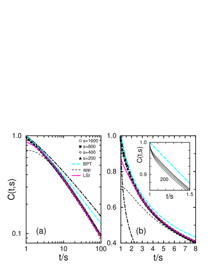
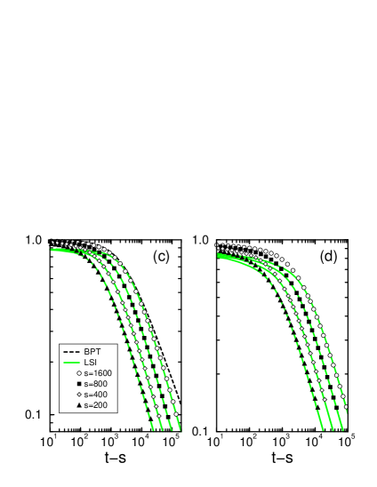
Figure 2: Two-time autocorrelation function $C(t,s)$ for the 2D Ising model and comparison with the LSI prediction (54,76). In (a) the scaling behaviour for $T=0$ is shown for a large range of values of $y=t/s$ and (b) redisplays the same data for smaller values of $y$. The inset compares the data for $y\approx 1$ and $s=[200,400,800,1600]$ with the closed approximation of BPT [16, 100]. The dash-dotted line in (a) is the second-order calculation from [78] and the dash-dotted line in (b) gives the result from [74], see text. The autocorrelation is re-plotted as a function of $t-s$ and compared to LSI for $T=0$ in (c) and for $T=1.5$ in (d). [55].

In figures 2 and 3 the degree of agreement between the numerical data and the prediction (54,76) is shown. Clearly, the system ages, as can be seen in figure 2cd, and there is excellent dynamical scaling for all models considered. For the Ising model, we show in figure 2ab the free-field approximation (56), labelled ‘app’, which only describes the data for rather large values of $y=t/s$. This is hardly surprising, since the model is known not to be described by a free field. On the other hand, we see that in all models the LSI predictions eqs. (54,76) give a good overall description over the whole range of the scaling variable, with the only exception of the relatively small region $t/s\lesssim 2-3$. It is conceivable that the patching procedure outlined in section 3 is not precise enough. It remains an open problem to derive a quantitatively precise formula which reproduces the numerical data over the entire range $1<y<\infty$.

Figure 3: Two-time autocorrelation function for the $2D$ $q$-states Potts model with $q=2$ (left), $q=3$ (middle) and $q=8$ (right) [76, 67]. The different data symbols correspond to different waiting times. The solid lines show the fits to the scaling prediction (76) based on local scale invariance.

On the other hand, the difficulty of achieving any quantitative agreement of an analytical approach and the numerical data is illustrated by comparing with the results of earlier attempts to find $C(t,s)$ in phase-ordering kinetics. Using Gaussian closure procedures, Bray, Puri and Toyoki (BPT) find for the O($n$)-model [16, 100, 91]

$$f_{C,{\rm BPT}}(y)=\frac{n}{2\pi}\left[B\left(\frac{1}{2},\frac{n+1}{2}\right)\right]^{2}\left(\frac{4y}{(y+1)^{2}}\right)^{d/4}\>{{}_{2}F_{1}}\left(\frac{1}{2},\frac{1}{2};\frac{n+2}{2};\left(\frac{4y}{(y+1)^{2}}\right)^{d/2}\right)~{}$$

where $B$ is Euler’s beta function [1]. While this form does follow the general trend of the data, especially if $y$ is not too large, but without reproducing them entirely, it mainly suffers from the disadvantage that it predicts the autocorrelation exponent $\lambda_{C}=d/2$ in disagreement with the data, see also figure 2c. Liu and Mazenko [74] and Mazenko [78] tried to remedy this by constructing more elaborate analytical schemes of which the BPT formula represents the lowest order. In particular, this leads for the $2D$ Ising model to fairly accurate values $\lambda_{C}=1.246(20)$ [74] and $\lambda_{C}=1.105\ldots$ [78] (Mazenko also showed [79] that $\lambda_{R}=\lambda_{C}$ in his scheme). However, the detailed behaviour for $f_{C}(y)$ deviates largely from the data, as can be seen from the dash-dotted lines in figure 2b for the prediction of [74] – in agreement with the earlier tests performed by Brown et al. [19] – and in figure 2a for the prediction of [78]. These examples illustrate the extreme difficulty of describing $C(t,s)$ theoretically. We consider it remarkable that local scale-invariance achieves, for the first time, a precise representation of the numerical data over almost the entire range of the scaling variable $y$.

A similar behaviour as for the Ising model is found for the Potts models with $q=3$ as well as $q=8$ [76]. This is the first time that the ageing behaviour and LSI of the autocorrelator was tested for a system which undergoes a first-order transition.

The examples presented here are the only ones which presently allow to test the extension $\mathfrak{age}_{d}\to\mathfrak{sch}_{d}\to\mathfrak{conf}_{d+2}$ of the local dynamical symmetry.

4.5 Bosonic contact and pair-contact processes

Two exactly solvable models allow to test the of LSI in situations when the stationary states are no longer equilibrium states, which requires a modification of the reduction formulæ to the deterministic part. See [61] and references therein for the motivation of these models, which are defined as follows [64, 83, 5]. Consider a set of particles of a single species $A$ which move on the sites of a $d$-dimensional hyper-cubic lattice. On any site one may have an arbitrary (non-negative) number of particles. Single particles may hop to a nearest-neighbour site with unit rate and in addition, the following single-site creation and annihilation processes are admitted

$$mA\stackrel{{\scriptstyle\mu}}{{\longrightarrow}}(m+1)A\;\;,\;\;pA\stackrel{{\scriptstyle\lambda}}{{\longrightarrow}}(p-\ell)A\;\;;\;\;\mbox{\rm with rates $\mu$ and $\lambda$}$$ (83)

where $\ell$ is a positive integer such that $|\ell|\leq p$. Consider the following special cases:

1. critical bosonic contact process: (bcp) $p=m=1$. Here only $\ell=1$ is possible. Furthermore the creation and annihilation rates are set equal $\mu=\lambda$.

2. critical bosonic pair-contact process: (bpcp) $p=m=2$. We fix $\ell=2$, set $2\lambda=\mu$ and define the control parameter

   $$\alpha:=\frac{3\mu}{2D}$$ (84)

Linear equations of motion for one- and two-point functions may be derived straightforwardly [64, 83, 5] and it follows that in both models the spatial average of the local particle-density $\int\!{\rm d}\boldsymbol{r}\,\rho(t,\boldsymbol{r})=\rho_{0}$ remains constant in time. Scaling occurs along the critical line [83]

$$\ell\lambda=\mu.$$ (85)

The physical behaviour of these models is indicated in the phase-diagramme figure 4. Whereas in the bcp the variance $\langle\rho^{2}(t,\boldsymbol{r})\rangle$ diverges as $t\to\infty$ for dimensions $d\leq 2$ but stays finite for $d>2$ such that one has the same behaviour along the critical line, in the bpcp there is a critical value $\alpha_{C}$ of the control parameter, given by

$$\frac{1}{\alpha_{C}}=2\int_{0}^{\infty}\!{\rm d}u\,\left(e^{-4u}I_{0}(4u)\right)^{d}$$ (86)

Specific values are $\alpha_{C}(3)\approx 3.99$, $\alpha_{C}(4)\approx 6.45$ and $\lim_{d\,\searrow\,2}\alpha_{C}(d)=0$. Now the variance $\langle\rho^{2}(t,\boldsymbol{r})\rangle$ stays finite on the critical line for $\alpha<\alpha_{C}$ but diverges otherwise.

Figure 4: Schematic phase-diagrammes for $D\neq 0$ of (a) the bosonic contact process and the bosonic pair-contact process in $d\leq 2$ dimensions and (b) the bosonic pair-contact process in $d>2$ dimensions. The absorbing region 1, where $\lim_{t\rightarrow\infty}\rho(\boldsymbol{x},t)=0$, is separated by the critical line eq. (85) from the active region 2, where $\rho(\boldsymbol{x},t)\to\infty$ as $t\to\infty$. Clustering along the critical line is indicated in (a) and (b) by full lines, but in the bosonic pair-contact process with $d>2$ the steady-state may also be homogeneous (broken line in (b)). These two regimes are separated by a multicritical point.

This means that at the multicritical point at $\alpha=\alpha_{C}$ there occurs a clustering transition such that for $\alpha<\alpha_{C}$ the systems evolves towards a more or less homogeneous state while for $\alpha\geq\alpha_{C}$ particles accumulate on very few lattice sites while the other ones remain empty. In contrast with the bosonic contact process, clustering occurs in some region of the parameter space for all values of $d$.

Solving the equations of motion with uncorrelated initial conditions yields the exact two-time autocorrelator (see table 1 and note that there is no scaling for $\alpha>\alpha_{C}$) which may also be written in an integral form

$$f_{C}(y)=\mathcal{C}_{0}\int_{0}^{1}\!{\rm d}\theta\,\theta^{a-b}(y+1-2\theta)^{-{d}/{2}}$$ (87)

quite similar to (56). While the relation $a=b$ still holds true for the bcp and the bpcp with $\alpha<\alpha_{C}$, that is no longer true for the bpcp at its multicritical point $\alpha=\alpha_{C}$ [5].

We now review how the formalism of LSI can be adapted to these models, following [6].

4.5.1 Bosonic contact process

From a field-theoretic point of view, the bcp can be described in terms of an order-parameter field $\phi$ and a response field $\widetilde{\phi}$, defined such that $\langle\phi(t,\boldsymbol{r})\rangle=\langle\widetilde{\phi}(t,\boldsymbol{r})\rangle=0$. The action [65, 98, 99] is again decomposed ${\cal J}[\phi,\widetilde{\phi}]={\cal J}_{0}[\phi,\widetilde{\phi}]+{\cal J}_{b}[\phi,\widetilde{\phi}]$ into a ‘deterministic’ part

$${\cal J}_{0}[\phi,\widetilde{\phi}]:=\int_{\mathbb{R}^{d}}\!{\rm d}\boldsymbol{R}\int_{0}^{\infty}\!{\rm d}u\>\left[\widetilde{\phi}(2\mathcal{M}\partial_{u}-\nabla^{2})\phi\right]$$ (88)

and which is manifestly Galilei-invariant, whereas the ‘noise’ now contains two contributions and is described by

$${\cal J}_{b}[\phi,\widetilde{\phi}]:=-\mu\int_{\mathbb{R}^{d}}\!{\rm d}\boldsymbol{R}\int_{0}^{\infty}\!{\rm d}u\>\left[{\widetilde{\phi}}^{2}(\phi+\rho_{0})\right].$$ (89)

where uncorrelated initial conditions are implied.

In what follows, some composite fields will be needed. Together with their scaling dimensions and their masses, they are listed in table 3.

field	scaling dimension	mass
$\phi$	$x$	$\cal M$
$\widetilde{\phi}$	$\widetilde{x}$	$-{\cal M}$
${\widetilde{\phi}}^{2}$	$\widetilde{x}_{2}$	$-2{\cal M}$
$\Upsilon:={\widetilde{\phi}}^{2}\phi$	$x_{\Upsilon}$	$-{\cal M}$
$\Sigma:={\widetilde{\phi}}^{3}\phi$	$x_{\Sigma}$	$-2{\cal M}$
$\Gamma:={\widetilde{\phi}}^{3}\phi^{2}$	$x_{\Gamma}$	$-{\cal M}$

Table 3: Scaling dimensions and masses of some composite fields.

For free fields one has $\widetilde{x}_{2}=2\widetilde{x}$, $x_{\Upsilon}=2\widetilde{x}+x$, $x_{\Sigma}=3\widetilde{x}+x$ and $x_{\Gamma}=3\widetilde{x}+2x$, but not necessarily so for interacting fields. On the other hand, from the Bargman superselection rules we expect that the masses of the composite fields as given in table 3 should remain valid for interacting fields as well.

As for magnets, the response function can reduced to a form which does not contain the noise explicitly [6]. The correlator becomes

$$C(t,s;\boldsymbol{r}-\boldsymbol{r}^{\prime}) = \left\langle\phi(t,\boldsymbol{r})\phi(s,\boldsymbol{r}^{\prime})\exp\left(-\mu\int\!{\rm d}\boldsymbol{R}\int\!{\rm d}u\>\widetilde{\phi}^{2}(u,\boldsymbol{R})\phi(u,\boldsymbol{R})\right)\right.$$

$$\left.~{}~{}\times\exp\left(-\mu\rho_{0}\int\!{\rm d}\boldsymbol{R}\int\!{\rm d}u\>\widetilde{\phi}^{2}(\boldsymbol{R},u)\right)\right\rangle_{0}$$

$$= -\mu\rho_{0}\int\!{\rm d}\boldsymbol{R}\int\!{\rm d}u\>\left\langle\phi(t,\boldsymbol{r})\phi(s,\boldsymbol{r}^{\prime})\widetilde{\phi}^{2}(u,\boldsymbol{R})\right\rangle_{0}$$

$$+\frac{\mu^{2}}{2}\int\!{\rm d}\boldsymbol{R}{\rm d}\boldsymbol{R}^{\prime}\int\!{\rm d}u{\rm d}u^{\prime}\>\left\langle\phi(t,\boldsymbol{r})\phi(s,\boldsymbol{r}^{\prime})\Upsilon(u,\boldsymbol{R})\Upsilon(u^{\prime},\boldsymbol{R}^{\prime})\right\rangle_{0}$$

using the field $\Upsilon$, see table 3. Hence the connected correlator is determined by three- and four-point functions of the noiseless theory.

The noiseless three-point response can be found from its covariance under the ageing algebra $\mathfrak{age}_{d}$ [6]

$$\langle\phi(t,\boldsymbol{r})\phi(s,\boldsymbol{r}^{\prime})\widetilde{\phi}^{2}(u,\boldsymbol{R})\rangle_{0} = (t-s)^{x-\frac{1}{2}\tilde{x}_{2}}(t-u)^{-\frac{1}{2}\tilde{x}_{2}}(s-u)^{-\frac{1}{2}\tilde{x}_{2}}$$ (91)

$$\times\exp\left(-\frac{\mathcal{M}}{2}\frac{(\boldsymbol{r}-\boldsymbol{R})^{2}}{t-u}-\frac{\mathcal{M}}{2}\frac{(\boldsymbol{r}^{\prime}-\boldsymbol{R})^{2}}{s-u}\right)\Psi_{3}(u_{1},v_{1})\Theta(t-u)\Theta(s-u)$$

with

$$u_{1} = \frac{u}{t}\cdot\frac{[(s-u)(\boldsymbol{r}-\boldsymbol{R})-(t-u)(\boldsymbol{r}^{\prime}-\boldsymbol{R})]^{2}}{(t-u)(s-u)^{2}}$$

$$v_{1} = \frac{u}{s}\cdot\frac{[(s-u)(\boldsymbol{r}-\boldsymbol{R})-(t-u)(\boldsymbol{r}^{\prime}-\boldsymbol{R})]^{2}}{(t-u)^{2}(s-u)}$$ (92)

and an undetermined scaling function $\Psi_{3}$. Hence the critical bcp is described by a free field-theory, one can expect that $x=\widetilde{x}=d/2$, hence $\tilde{x}_{2}=d$, $x_{\Upsilon}=\frac{3}{2}d$ for the composite fields. Therefore the autocorrelator takes the general form $C(t,s)=s^{1-d/2}g_{1}(t/s)+s^{2-d}g_{2}(t/s)$ and for $d>2$ the second term, which comes from the four-point function, merely furnishes a finite-time correction to scaling. Now, if one chooses in eq. (91) [87]

$$\Psi_{3}(u_{1},v_{1})=\Xi\left(\frac{1}{u_{1}}-\frac{1}{v_{1}}\right)$$ (93)

where $\Xi$ remains an arbitrary function, then

$$C(t,s) = -\mu\rho_{0}s^{\frac{d}{2}+1-x-\frac{1}{2}\tilde{x}_{2}}(t/s-1)^{\frac{1}{2}\tilde{x}_{2}-x-\frac{d}{2}}$$ (94)

$$\times\int_{0}^{1}\!{\rm d}\theta\,[(t/s-\theta)(1-\theta)]^{\frac{d}{2}-\frac{1}{2}\tilde{x}_{2}}\boldsymbol{\Psi}\left(\frac{t/s+1-2\theta}{t/s-1}\right)$$

where the function $\boldsymbol{\Psi}$ is defined by

$$\boldsymbol{\Psi}(w)=\int_{\mathbb{R}^{d}}\!{\rm d}\boldsymbol{R}\,\exp\left(-\frac{\mathcal{M}w}{2}\boldsymbol{R}^{2}\right)\Xi(\boldsymbol{R}^{2})$$ (95)

and the LSI-prediction for the critical point (56) is indeed recovered. The specific result for the bcp as listed in table 1 follows for $\boldsymbol{\Psi}(w)=\Psi_{0}w^{-1-a}$.

4.5.2 Bosonic pair-contact process

In this case, a new ingredient will be needed. The action now reads [65] ${\cal J}[\phi,\widetilde{\phi}]={\cal J}_{0}[\phi,\widetilde{\phi}]+{\cal J}_{b}[\phi,\widetilde{\phi}]$ with the ‘deterministic’ part

$${\cal J}_{0}[\phi,\widetilde{\phi}]:=\int_{\mathbb{R}^{d}}\!{\rm d}\boldsymbol{R}\int_{0}^{\infty}\!{\rm d}t\>\left[\widetilde{\phi}(2\mathcal{M}\partial_{t}-\nabla^{2})\phi-\alpha\widetilde{\phi}^{2}\phi^{2}\right].$$ (96)

and the noise part

$${\cal J}_{b}[\phi,\widetilde{\phi}] = \int_{\mathbb{R}^{d}}\!{\rm d}\boldsymbol{R}\int_{0}^{\infty}\!{\rm d}u\>\left[-\alpha\rho_{0}^{2}\widetilde{\phi}^{2}-2\alpha\rho_{0}\widetilde{\phi}^{2}\phi-\mu\widetilde{\phi}^{3}\phi^{2}-2\mu\rho_{0}\widetilde{\phi}^{3}\phi-\rho_{0}^{2}\widetilde{\phi}^{3}\right]$$ (97)

The representations of $\mathfrak{age}_{d}$ or $\mathfrak{sch}_{d}$ considered in sections 2 and 3 can no longer be used, since the equation of motion associated to $J_{0}$ is non-linear, viz.

$$2\mathcal{M}\partial_{t}\phi(t,\boldsymbol{r})=\nabla^{2}\phi(t,\boldsymbol{r})-g\phi^{2}(t,\boldsymbol{r})\widetilde{\phi}(t,\boldsymbol{r})$$ (98)

Rather, new representations of $\mathfrak{age}_{d}$ and $\mathfrak{sch}_{d}$ must be constructed which take into account that $g$ is a dimensionful quantity which transforms under local scale-transformations [96, 6] but the generators will not be written down explicitly here for the sake of brevity. It can then be shown that (i) eq. (98) is Schrödinger-invariant for any value of $d$ and (ii) the Bargman superselection rules (37) still apply.

Turning to the calculation of the autocorrelation function, one must consider five possible contributions. It turns out [6] that the results of table 1 for $f_{C}(y)$ in the bpcp can be reproduced from the single term

$$C(t,s)=\alpha\rho_{0}^{2}\int_{\mathbb{R}^{d}}\!{\rm d}\boldsymbol{R}\int_{0}^{\infty}\!{\rm d}u\>\left\langle\phi(t,\boldsymbol{r})\phi(s,\boldsymbol{r})\widetilde{\phi}^{2}(u,\boldsymbol{R})\right\rangle_{0}$$ (99)

The required $\mathfrak{age}_{d}$-invariant three-point function now reads, where $x=a+1=d/2$ is read off from the response function [6]

$$\left\langle\phi(t,\boldsymbol{r})\phi(s,\boldsymbol{r}^{\prime})\tilde{\phi}^{2}(u,\boldsymbol{R})\right\rangle_{0} = (t-s)^{x-\frac{1}{2}\tilde{x}_{2}}(t-u)^{-\frac{1}{2}\tilde{x}_{2}}(s-u)^{-\frac{1}{2}\tilde{x}_{2}}$$ (100)

$$\times\exp\left(-\frac{\mathcal{M}}{2}\frac{(\boldsymbol{r}-\boldsymbol{R})^{2}}{t-u}-\frac{\mathcal{M}}{2}\frac{(\boldsymbol{r}^{\prime}-\boldsymbol{R})^{2}}{s-u}\right)\tilde{\Psi}_{3}(u_{1},v_{1},\beta_{1},\beta_{2},\beta_{3})$$

with

$$u_{1} = \frac{u}{t}\cdot\frac{[(s-u)(\boldsymbol{r}-\boldsymbol{R})-(t-u)(\boldsymbol{r}^{\prime}-\boldsymbol{R})]^{2}}{(t-u)(s-u)^{2}}$$ (101)

$$v_{1} = \frac{u}{s}\cdot\frac{[(s-u)(\boldsymbol{r}-\boldsymbol{R})-(t-u)(\boldsymbol{r}^{\prime}-\boldsymbol{R})]^{2}}{(t-u)^{2}(s-u)}$$ (102)

$$\beta_{1} = \frac{1}{s_{2}}\cdot\frac{\alpha^{1/y}}{(t-u)^{2}},\;\;\beta_{2}=\frac{1}{s_{2}}\cdot\frac{\alpha^{1/y}}{(s-u)^{2}},\;\;\beta_{3}=\alpha^{1/y}s_{2}$$ (103)

$$s_{2} = \frac{1}{t-u}+\frac{1}{u}$$ (104)

where $y$ is the scaling dimension of $g$. Consider the following choice for $\tilde{\Psi}_{3}$ [6]

$$\tilde{\Psi}_{3}(u_{1},v_{1},\beta_{1},\beta_{2},\beta_{3})=\Xi\left(\frac{1}{u_{1}}-\frac{1}{v_{1}}\right)\left[-\frac{(\sqrt{\beta_{1}}-\sqrt{\beta_{2}})\sqrt{\beta_{3}}}{\beta_{3}-\sqrt{\beta_{2}\beta_{3}}}\right]^{(a-b)}$$ (105)

where the scaling function $\Xi$ was already given in eq. (93), as for the bosonic contact process. We now have to distinguish the two different cases: first, if $\alpha<\alpha_{C}$ then $a=b$ [5] and we are back to the expressions found for the bcp. Second, if $\alpha=\alpha_{C}$ then $a-b=d/2-1$ for $2<d<4$ and $a-b=1$ for $d>4$, respectively [5]. Identifying $\widetilde{x}_{2}=2(b-a)+d$, one finally obtains

$$C(t,s) = s^{-b}(y-1)^{(b-a)-a-1}\int_{0}^{1}\!{\rm d}\theta\,[(t/s-\theta)(1-\theta)]^{a-b}$$ (106)

$$\times\boldsymbol{\Psi}\left(\frac{t/s+1-2\theta}{t/s-1}\right)\left[\frac{\theta(t/s-1)}{(t/s-\theta)(1-\theta)}\right]^{a-b}$$

The specific results of table 1 for the bpcp are recovered if one uses the free-field form $\boldsymbol{\Psi}(w)=\Psi_{0}w^{-1-a}$.

5 Growth models and an outlook towards $z\neq 2$

A different class of non-equilibrium models considers the ballistic deposition of particles on a surface. The state of this surface may be described in terms of a height variable $h(t,\boldsymbol{r})$. For irreversible deposition, the system clearly never arrives at an equilibrium state. Working in the frame co-moving with the mean surface height, the simplest kinetic equation one may write in the case without mass conservation is the well-known Edwards-Wilkinson (ew) model [35]

$$\partial_{t}h(t,\boldsymbol{r})=D\nabla^{2}h(t,\boldsymbol{r})+\eta(t,\boldsymbol{r})$$ (107)

However, if mass conservation must be taken into account, one might rather consider the Mullins-Herring (mh) model, see [80, 102]

$$\partial_{t}h(t,\boldsymbol{r})=-D(\nabla^{2})^{2}h(t,\boldsymbol{r})+\eta(t,\boldsymbol{r})$$ (108)

Following [90], the following types of gaussian noise with vanishing first moment $\langle\eta(t,\boldsymbol{r})\rangle=0$ will be considered:

1. non-conserved, short-ranged $\langle\eta(t,\boldsymbol{r})\eta(s,\boldsymbol{r}^{\prime})\rangle=2D\delta(\boldsymbol{r}-\boldsymbol{r}^{\prime})\delta(t-s)$.

2. non-conserved, long-ranged $\langle\eta(t,\boldsymbol{r})\eta(s,\boldsymbol{r}^{\prime})\rangle=2D|\boldsymbol{r}-\boldsymbol{r}^{\prime}|^{2\rho-d}\delta(t-s)$ and $0<\rho<d/2$.

3. conserved, short-ranged $\langle\eta(t,\boldsymbol{r})\eta(s,\boldsymbol{r}^{\prime})\rangle=-2D\nabla_{\boldsymbol{r}}^{2}\delta(\boldsymbol{r}-\boldsymbol{r}^{\prime})\delta(t-s)$.

Then the following models were studied in [90]:

1. ew1: eq. (107) with the non-conserved noise (a).

2. ew2: eq. (107) with the non-conserved, long-ranged noise (b).

3. mh1: eq. (108) with the non-conserved noise (a).

4. mh2: eq. (108) with the non-conserved, long-ranged noise (b).

5. mhc: eq. (108) with the conserved noise (c) [9].

To these, one may add the spherical model with a conserved order-parameter (model B dynamics) [71, 77, 95, 9] which for $d>4$ reduces to mhc. For $2<d<4$ an explicit, if rather lengthy, expression for $C(t,s)$ and its explanation in terms of LSI has been derived [9].

In the models ew1 and mhc the noise is in agreement with detailed balance while for the other models it is not. Solving the linear equations (107) and (108) is straightforward and the two-time autocorrelations are listed in table 1. The result quoted for the mhc model is only valid for $d>2$ as stated; for $d=2$ the scaling function becomes $f_{C}(y)=2D\ln[(y-1)/(y+1)]$ [9]. Detailed simulations show that the correlation and response functions of the well-known Family model [37] and of a variant of it are perfectly described by the ew1 model and hence should be in the same universality class [90].

5.1 Local scale-invariance for $z=4$

In line with the approach taken for $z=2$, we shall consider the dynamical symmetries of the ‘deterministic’ part of these equations and then try to prove a generalization of the Bargman superselection rules such that the results can be extended to the full noisy system. Consider the ‘Schrödinger equation’ ${\cal S}_{4}\psi=0$ where the ‘Schrödinger operator’ is defined as

$$\mathcal{S}_{4}:=-\mu\partial_{t}+\frac{1}{16}\partial_{r}^{4}$$ (109)

The parameter $\mu$ is the analogue of the mass $\mathcal{M}$ for the case $z=2$ (and should not be confused with the exponent $\mu$ defined in section 3). Dynamical symmetries of this kind of simple linear equation have been constructed for any given $z$ [50]. For the special case $z=4$, some of the generators read in $d=1$ dimensions as follows (see [90, 9] for the extension to $d>1$)

$$X_{-1} = -\partial_{t}$$

$$Y_{-1/4} = -\partial_{r}$$

$$X_{0} = -t\partial_{t}-\frac{1}{4}r\partial_{r}-\frac{x}{4}$$

$$X_{1} = -t^{2}\partial_{t}-\frac{1}{2}tr\partial_{r}-\frac{x}{2}t-\mu r^{2}\partial_{r}^{-2}+4\gamma r\partial_{r}^{-3}-6\gamma\partial_{r}^{-4}$$ (110)

$$Y_{3/4} = -t\partial_{r}-4\mu r\partial_{r}^{-2}+8\gamma\partial_{r}^{-3}$$

where $\gamma$ is a parameter and the ‘derivative’ $\partial_{r}^{a}$ satisfies the formal properties $\partial_{r}^{a}\partial_{r}^{b}=\partial_{r}^{a+b}$ and $[\partial_{r}^{a},r]=a\partial_{r}^{a-1}$ [50]. Then it is straightforward to check that

$${}[{\cal S}_{4},Y_{-1/4}]\>=\>[{\cal S}_{4},Y_{3/4}]\>=\>[{\cal S}_{4},R^{(i,j)}]\>=\>0\;\;,\;\;{}[{\cal S}_{4},X_{0}]=-{\cal S}_{4}$$ (111)

and

$$[\mathcal{S}_{4},X_{1}]\>=\>-2t\mathcal{S}_{4}+\frac{\mu}{2}\left(x-\frac{3}{2}+\frac{2\gamma}{\mu}\right)$$ (112)

and the commutator of ${\cal S}_{4}$ with all other generators (5.1) vanishes. As before for Schrödinger and conformal invariance, this means the generators (5.1) act as dynamical symmetry operators provided that the scaling dimension of the solution $\psi$ of ${\cal S}_{4}\psi=0$ is $x=3/2-2\gamma/\mu$. As before, a scaling operator is called quasiprimary [12, 50, 59] if its infinitesimal transformation is given by (5.1). Quasiprimary operators are now characterized by the triplett $(x,\gamma/\mu,\mu)$, rather than the pair $(x,{\cal M})$ as it is the case for Schrödinger-invariance. These ’quantum numbers’ are connected to the critical exponents of the model at hand. It appears that $x$ and $\gamma/\mu$ are universal numbers, while $\mu$ (as is $\cal M$) is dimensionful and must be non-universal.

The two-point function $F_{0}^{(2)}$ built from two quasiprimary scaling operators $\phi$ and $\widetilde{\phi}$ has the form [50, 90, 9]

$$\left\langle\phi(t,\boldsymbol{r})\widetilde{\phi}(s,\boldsymbol{r}^{\prime})\right\rangle_{0}=\delta_{x,\widetilde{x}}\,\delta_{\gamma,\widetilde{\gamma}}\,\delta_{\mu,\widetilde{\mu}}\>(t-s)^{-x/2}\varphi\left(|\boldsymbol{r}-\boldsymbol{r}^{\prime}|(t-s)^{-1/4}\right)$$ (113)

where the scaling function is given by $\varphi(u)=\sum_{m=0}^{3}c_{m}\varphi^{(m)}(u)$ where

$$\varphi^{(m)}(u)=\sum_{n=0}^{\infty}b_{n}^{(m)}u^{4(n-1)+m+1}\;\;,\;\;b_{n}^{(m)}=\frac{(-16\mu)^{n}\Gamma\left(1+m\right)\Gamma\left(n+\frac{m}{4}-\frac{\gamma}{\mu}\right)}{\Gamma\left(4(n-1)+m+2\right)\Gamma\left(\frac{m}{4}-\frac{\gamma}{\mu}\right)}.$$ (114)

Here, the coefficients $c_{m}$ are left arbitrary (although further constraints may be imposed on them by requiring that the scaling function $\varphi(u)\to 0$ as $u\to\infty$).

In order to break time-translation invariance as required for applications to ageing, we introduce a time-dependent potential $v(t)$ and consider the equation

$$\partial_{t}\phi=-\frac{1}{16\mu}\nabla_{\boldsymbol{r}}^{2}\Big{(}-\nabla_{\boldsymbol{r}}^{2}\phi+v(t)\phi\Big{)}+\eta(t,\boldsymbol{r})+j(t,\boldsymbol{r})$$ (115)

with a gaussian white noise $\eta(t,\boldsymbol{r})$ and a perturbation $j(t,\boldsymbol{r})$ for the calculation of responses. The potential can be eliminated through a gauge transformation [9]

$$\phi(t,\boldsymbol{r})=\exp\left(-\frac{1}{16\mu}\int_{0}^{t}{\rm d}\tau v(\tau)\nabla_{\boldsymbol{r}}^{2}\right)\psi(t,\boldsymbol{r})$$ (116)

In contrast to the case $z=2$, we now assume that for $t\to\infty$ $\int_{0}^{t}\!{\rm d}\tau\,v(\tau)\sim t^{\digamma}$ in order to ensure scaling behaviour for large times. This defines the new parameter $\digamma$ but we warn the reader that this parameter should not be confused with the one used in eq. (44).

Now, progress is possible if the deterministic part reduces to a linear equation. Then Wick’s theorem holds which permits to derive analogous reduction formulæ as in the case $z=2$. For a fully disordered initial state with $\langle\phi(0,\boldsymbol{R})\phi(0,\boldsymbol{R}^{\prime})\rangle=a_{0}\delta(\boldsymbol{R}-\boldsymbol{R}^{\prime})$ the response function is then explicitly given by [90, 9]

$$R(t,s;\boldsymbol{r}) = F_{0}^{(2)}(t,s;\boldsymbol{r})$$ (117)

$$= (t-s)^{-x/2}\sum_{m=0}^{3}c_{m}u^{m+1}\sum_{k,n=0}^{\infty}b_{n,k}^{(m)}\left[-\frac{\kappa_{0}(t^{\digamma}-s^{\digamma})}{16\mu(t-s)^{1/2}}\right]^{k}u^{4(n-1)-2k}$$

with the scaling variable $u=|\boldsymbol{r}|(t-s)^{-1/4}$ and the coefficients $b_{n,k}^{(m)}$, which are given by

$$b_{n,k}^{(m)}=\frac{1}{k!}\frac{\Gamma(4(n-1)+m+2)}{\Gamma(2k-4(n-1)-m)}\,b_{n}^{(m)}$$ (118)

which is perfectly consistent with the available information from the several mh models introduced above [90] and also for the spherical model with a conserved order-parameter [9].

On the other hand, the correlation function becomes, with $t>s$

$$C(t,s;\boldsymbol{r}) = \frac{a_{0}}{2}\int_{\mathbb{R}^{d}}\!{\rm d}\boldsymbol{R}\,F_{0}^{(3)}(t,s,0;\boldsymbol{r},\boldsymbol{0},\boldsymbol{R})$$ (119)

$$-\frac{T}{16\mu}\int_{0}^{s}\!{\rm d}\tau\int_{\mathbb{R}^{d}}\!{\rm d}\boldsymbol{R}\,F_{0}^{(3)}(t,s,\tau;\boldsymbol{r},\boldsymbol{0},\boldsymbol{R})$$

where the deterministic three-point function is
$F_{0}^{(3)}(t,s,\tau;\boldsymbol{r},\boldsymbol{r}^{\prime},\boldsymbol{R}):=\langle\phi(t,\boldsymbol{r})\phi(s,\boldsymbol{r}^{\prime})\widetilde{\phi}^{2}(\tau,\boldsymbol{R})\rangle_{0}$. If the deterministic part reduces to a linear equation, then Wick’s theorem leads to [9]

$$F_{0}^{(3)}(t_{1},t_{2},t_{3};\boldsymbol{r}_{1},\boldsymbol{r}_{2},\boldsymbol{r}_{3})=2F_{0}^{(2)}(t_{1},t_{3};\boldsymbol{r}_{1}-\boldsymbol{r}_{3})F_{0}^{(2)}(t_{2},t_{3};\boldsymbol{r}_{2}-\boldsymbol{r}_{3})$$ (120)

where $F_{0}^{(2)}$ can be taken from eq. (117). Carrying out the (rather long) calculation then allows to fully reproduce all results listed in table 1 for the models with $z=4$. At least for the models studied so far with $z=4$, the relation $a=a^{\prime}$ was empirically found to be satisfied. That is not surprising in view of the simple linear equation satisfied by the order-parameter field $\phi$.

The mh models considered in this section are, together with the critical spherical model with a conserved order-parameter, the first analytically solved examples with $z\neq 2$ where local scale-invariance could be fully confirmed. These examples make it in particular clear that the height of the surface in growth processes is a natural candidate for being described by a quasiprimary scaling operator of local scale-invariance.

5.2 ‘Conformal invariance’ for $z\neq 1,2$ ?

We finish with a short speculation on how one might construct an analogy of the extension $\mathfrak{sch}_{d}\to\mathfrak{conf}_{d+2}$ discussed in section 2.3. By analogy, one might try to consider the ‘mass’ $\mu$ as a further variable and thus try to find analogues to the operators $V_{-}$ and $N$ described in section 2.3. If we very naïvely generalise $V_{-}$ and $N$ from the case $z=2$ and define

$$V_{-}=-{\rm i}\partial_{\mu}\partial_{r}^{3}+4{\rm i}r\partial_{t}\;\;,\;\;N=-t\partial_{t}-1-\mu\partial_{\mu}$$ (121)

then it can be checked that both commutators $[{\cal S}_{4},N]$ and $[{\cal S}_{4},V_{-}]$ vanish. This already implies that these two operators describe new, non-trivial symmetries and are appropriate candidates for a possible extension of the algebra freely generated from the minimal set $\{X_{-1},X_{0},X_{1},Y_{-1/4},Y_{3/4}\}$. At this stage, the algebraic structure of such an extension is not clear at all; see [50] for the discussion of some other difficulties which may arise when one wishes to find the algebra satisfied by local scale-transformations with $z\neq 1,2$ and such that they can be symmetries of physically non-trivial equations – which in the context of ${\cal S}_{4}$ would mean that $\mu\neq 0,\infty$.

Of course, the central question whether an analogue of Bargman superselection rules exists is not even addressed. We hope to come back to this elsewhere, see [11].

6 Conclusions

We have considered how local scale-invariance might be used in order to arrive at an explicit prediction for the two-time autocorrelation function of phase-ordering kinetics (as well as for non-equilibrium critical dynamics in those special cases where $z=2$) capable to reproduce simulational data. In comparison with the two-time response function, whose functional form simply follows from the assumed covariance of the quasiprimary scaling operators of the ageing algebra $\mathfrak{age}_{d}$, the calculation of $C(t,s)$ does require conceptually important extensions. First, the explicit reduction from a stochastic Langevin equation to a deterministic equation is needed since a simple covariance argument for $C(t,s)$ would have led to a vanishing autocorrelation because of the Bargman superselection rules, see [87]. Second, invariance under $\mathfrak{age}_{d}$ alone does not seem to lead to any predictions for the autocorrelator, with the exception of the exponent relation $\lambda_{C}=\lambda_{R}$ between the autocorrelation and the autoresponse exponents for the case of fully disordered initial conditions. Therefore, the third required extension concerns the dynamical symmetry algebra itself

$$\mathfrak{age}_{d}\to\mathfrak{sch}_{d}\to\mathfrak{conf}_{d+2}$$ (122)

which then allows to reduce the scaling function $f_{C}(y)$ to the linear combination of two known functions. We have also described some subleties in the precise definition of quasiprimary scaling operators and the several scaling dimensions ($x,\xi,\digamma$) on which they depend.

Besides several confirmations of the first two steps from analytically solved models with an underlying free-field theory, remarkably there is strong evidence from two-dimensional kinetic Ising and Potts models in favour of the last extension to a new type of conformal invariance, at least for quenches to $T<T_{c}$, where $z=2$.

It might be useful here to list some of the important open problems.

1. A more systematic approach replacing the glueing procedure outlined in section 3.2 (and the appendix) should be found, hopefully leading to full agreement between the theory and the data.

2. The Galilei- and other local scale-invariances of non-linear partial differential equations must be studied. Present results [96, 6] require Galilei-invariance for all times which is too strong a requirement to be able to include the usual kind of Langevin equations [63]. A new kind of asymptotic Galilei-invariance, only valid in the scaling regime (3), would be enough and might be more flexible, but remains to be constructed.

   The importance of Galilei-invariance implies that models without a spatial structure such as the zero-range process [36, 47] cannot be expected to satisfy a local scale-invariance. On the other hand, it might be of interest to inquire whether driven diffusive systems [93] may possess some form of local scale-invariance.

3. Analytical tests of local scale-invariance only exist for a rather simple kind of solvable systems, with an underlying free-field theory. The calculation of two-time observables in more rich integrable systems would certainly provide most useful information.

4. Present tests of local scale-invariance have been limited mainly to systems with $z=2$ or focused on the autoresponse whose form does not depend on directly on $z$. Therefore important aspects of the theory as outlined in [50] have not yet been tested. We hope that the consideration of phase-ordering in disordered Ising models [84, 58] and in certain models with long-range interactions [24, 10] where $z$ depends continuously on the control parameters of the model, will allow to do this.

5. A central point for the applicability to stochastic Langevin equations is the derivation of extensions of the Bargman superselection rules to $z\neq 2$. Work along these lines is in progress [11].

6. Is there a way to formulate an infinite-dimensional extension of the local scale-transformations considered here, in analogy with $2D$ conformal invariance at equilibrium [12, 25]? At the time of writing, there merely exist some isolated mathematical results on equations with an infinite-dimensional dynamical symmetry, on the algebraic structure of the related Lie algebras and their vertex operator representations [29, 89, 101]. What would be the physical signatures of such a symmetry which could be tested in specific models ?

7. Dynamical scaling combined with reparametrization invariance has been considered for glasses where, because of logarithmic scaling, the effective dynamical exponent $z\to\infty$, see [27, 28] and references therein. Will there be a way to relate these distinct approaches of local scaling ?

All in all, local scale-invariance may offer an approach complementary to numerical simulation and the field-theoretical renormaliztion group (so far restricted to non-equilibrium critical dynamics [21]). The presently available evidence suggests the possibility of establishing a hidden dynamical symmetry which had not been suspected and, if proven correct, could simplify considerably the description of the non-equilibrium dynamics of many-body systems.

Appendix.

We explain how to extend the description of the three-point function $\langle\Phi(t)\Phi(s)\widetilde{\Phi}^{2}(u)\rangle_{0}$ to the region where $t\approx s$ and local scale-invariance can no longer be used. Throughout, we restrict to the case of phase-ordering ($T<T_{c}$) and we shall derive eq. (76). Our physical criterion is the requirement that the two-time autocorrelator be symmetric in $t$ and $s$ and furthermore be non-singular as $t-s\to 0$. From the from eq. (49) this leads to the following form of the scaling function $\Psi(\rho)$, since $x-\widetilde{x}_{2}+2\xi-2\widetilde{\xi}_{2}=\lambda_{C}-d/2$

$$\Psi(\rho)=\rho^{\lambda_{C}-d/2}\sum_{n=0}^{\infty}\Psi_{n}\rho^{2n}$$ (A1)

where the $\Psi_{n}$ are constants. Because of the Yeung-Rao-Desai inequality $\lambda_{C}\geq d/2$ [103] this expression will increase with $\rho$ for sufficiently small values of $\rho$, whereas the LSI-prediction eq. (72) gives a divergence at $\rho=0$, unless $a^{\prime}\leq 0$ which in any case is incompatible with the explicit results in many models, see section 4 and [61, 62]. We expect (A1) to be valid for sufficiently small values of $\rho$ and to change to the form predicted by LSI if $\rho$ becomes larger than some minimal value $\varepsilon$. For $\rho$ sufficiently small, we may approximate (72) as follows

$$\Psi_{\rm scal}(\rho) \simeq \psi_{0}\rho^{\lambda_{C}-d/2-2a^{\prime}}\left(1-\frac{2\lambda_{C}-d-2a^{\prime}}{1+\lambda_{C}-d/2-2a^{\prime}}{\cal M}\rho+\ldots\right)$$ (A2)

$$+\psi_{1}{\cal M}^{2a^{\prime}+d/2-\lambda_{C}}+\ldots$$

which should be valid for $\rho\gtrsim\varepsilon$. Since in phase-ordering one usually treats systems of class S where $a=a^{\prime}=1/z=1/2$ and $\lambda_{C}\geq d/2$, all the terms retained here are needed to have a consistent expansion as $\rho\to 0$.

If the cross-over point $\varepsilon$ is sufficiently small, only the leading term in (A1) is needed. We construct a scaling function $\Psi(\rho)$ for all $\rho\geq 0$ by requiring that the branches (A1) and (A2) meet continuously at $\rho=\varepsilon$. This condition fixes $\Psi_{0}=\Psi_{0}(\varepsilon)$ and we find, to this order

$$\Psi_{0}(\varepsilon) = \psi_{0}\varepsilon^{-2a^{\prime}}-\psi_{0}{\cal M}\frac{2\lambda_{C}-d-2a^{\prime}}{1+\lambda_{C}-d/2-2a^{\prime}}\varepsilon^{1-2a^{\prime}}$$ (A3)

$$+\psi_{1}{\cal M}^{2a^{\prime}+d/2-\lambda_{C}}\varepsilon^{d/2-\lambda_{C}}$$

The required scaling function $\boldsymbol{\Psi}$ is given by

$$\boldsymbol{\Psi}(w) = \int_{\mathbb{R}^{d}}\!{\rm d}\boldsymbol{R}\>e^{-{\cal M}w\boldsymbol{R}^{2}/2}\,\Psi\left(\frac{\boldsymbol{R}^{2}}{2}\right)$$ (A4)

$$= 2^{d/2-1}S_{d}\int_{0}^{\infty}\!{\rm d}u\>u^{d/2-1}\,e^{-{\cal M}wu}\,\Psi(u)$$

$$= 2^{d/2-1}S_{d}\left(\int_{0}^{\infty}\!{\rm d}u\>u^{d/2-1}\,e^{-{\cal M}wu}\,\Psi_{\rm LSI}(u)\right.$$

$$+\left.\int_{0}^{\varepsilon}\!{\rm d}u\>u^{d/2-1}\,e^{-{\cal M}wu}\left(\Psi_{0}(\varepsilon)u^{\lambda_{C}-d/2}-\Psi_{\rm scal}(u)\right)\right)$$

$$=: 2^{d/2-1}S_{d}\left(I_{0}+I_{1}+I_{\varepsilon}\right)$$

where $S_{d}$ is the surface of the sphere in $d$ dimensions, $I_{0,1}$ are proportional to $\psi_{0,1}$, $\Psi_{\rm LSI}$ is the LSI-prediction given in (72) and eqs. (A2) and (A3) were used. In the third line the range of integration was split into the intervals $[0,\varepsilon]$ and $[\varepsilon,\infty]$ and the leading term from (A1) was used in the first subinterval. The terms $I_{0,1}$ refer to the two independent solutions for $\Psi(\rho)$ in eq. (72). They can be calculated using the identity

$$\int_{0}^{\infty}\!{\rm d}u\>u^{\alpha-1}\,e^{-\omega u}\>{{}_{1}F_{1}}(A,B;-u)=\frac{\Gamma(\alpha)}{\omega^{\alpha}}\,{{}_{2}F_{1}}\left(A,\alpha;B;-\frac{1}{\omega}\right)$$ (A5)

This already gives the first two lines in (76). The terms contained in $I_{\varepsilon}$ are calculated from the identity

$$\int_{0}^{1}\!{\rm d}u\>u^{\beta-1}\,e^{-\omega u}=\omega^{-\beta}\,\gamma(\beta,\omega)$$ (A6)

where $\gamma(\beta,\omega)$ is an incomplete gamma function [1]. Combining the various terms and setting

$$A:=\psi_{0}2^{d/2-1}S_{d}{\cal M}^{2a^{\prime}-\lambda_{C}}\;\;,\;\;B:=\psi_{1}2^{d/2-1}S_{d}{\cal M}^{2a^{\prime}-\lambda_{C}}\;\;,\;\;E:={\cal M}\varepsilon$$ (A7)

we finally arrive at eq. (76) in the text.

Inserting this result into the two-time autocorrelation function eq. (54), the amplitude $C_{\infty}=\boldsymbol{\Psi}(1)=\lim_{y\to\infty}y^{\lambda_{C}/2}C(ys,s)$ is given by

$$C_{\infty} = A\left\{\Gamma(\lambda_{C}-2a^{\prime})\>{{}_{2}F_{1}}(2\lambda_{C}-d-2a^{\prime},\lambda_{C}-2a^{\prime};1+\lambda_{C}-d/2-2a^{\prime};-1)\right.$$ (A8)

$$+E^{-2a^{\prime}}\gamma(\lambda_{C},E)-\gamma(\lambda_{C}-2a^{\prime},E)$$

$$+\left.E^{1-2a^{\prime}}\frac{2\lambda_{C}-d-2a^{\prime}}{1+\lambda_{C}-d/2-2a^{\prime}}\left[E^{2a^{\prime}-1}\gamma(\lambda_{C}+1-2a^{\prime},E)-\gamma(\lambda_{C},E)\right]\right\}$$

$$+ B\left\{\Gamma(d/2)\>{{}_{2}F_{1}}(\lambda_{C}-d/2,d/2;1+2a^{\prime}+d/2-\lambda_{C};-1)\right.$$

$$\left.+E^{d/2-\lambda_{C}}\gamma(\lambda_{C},E)-\gamma(d/2,E)\right\}$$

which gives a useful technique to fix one of the free parameters $A,B,E$ in terms of the other two. Indeed, in order to find $C_{\infty}$ empirically from numerical data, it is considerably more precise to plot $C(ys,s)y^{-\lambda_{C}/2}(y-1)^{\lambda_{C}}$ over against $y$, rather than the simplistic $C(ys,s)y^{\lambda_{C}/2}$.

The opposite limit $\lim_{y\to 1}C(ys,s)=C(t,t)=C_{1}$ exists if $2a^{\prime}\leq 1$ and then becomes

$$C_{1}=\Gamma(\lambda_{C})2^{-\lambda_{C}}\left\{AE^{-2a^{\prime}}\left[1-E\frac{2\lambda_{C}-d-2a^{\prime}}{1+\lambda_{C}-d/2-2a^{\prime}}\left(1-\delta_{2a^{\prime},1}\right)\right]+BE^{d/2-\lambda_{C}}\right\}~{}~{}$$ (A9)

which for finite $E$ is indeed a finite constant.

For a free field, one has $\lambda_{C}=d/2$. If one takes $A=0$ and $B>0$, one recovers $\boldsymbol{\Psi}(w)=B\Gamma(d/2)w^{-d/2}$, as it should be.

If one should find that the description of $\Psi(\rho)$ for $\rho\leq\varepsilon$ merely by the lowest order-term is not sufficiently precise, further terms from (A1) may be included (balanced by the higher-order terms of the expansion of $\Psi_{\rm LSI}(\rho)$) and the coefficients $\Psi_{n}$ fixed by requiring also the continuity of the respective derivatives of $\Psi(\rho)$ at $\rho=\varepsilon$.

Acknowledgements:

It is a pleasure to thank the organisers of the workshop Principles of the dynamics of non-equilibrium systems and Isaac Newton Institute for warm hospitality in a stimulating environnement; A.J. Bray, L. Berthier, J.L. Cardy, J.P. Garrahan, A. Lefèvre, S. Majumdar, G. Odor, V. Rittenberg, B. Schmittmann, G.M. Schütz, P. Sollich for fruitful discussions; A. Picone, M. Pleimling, A. Röthlein, S. Stoimenov, J. Unterberger for the year-long collaborations which lead to the results reviewed here and E. Lorenz and W. Janke for communicating their results before publication, discussions and for sending figure 3. We also thank A. Gambassi and H. Hinrichsen for their critical but constructive comments on LSI, forcing us to lay the foundations of the theory in a more precise way. FB acknowledges the support by the Deutsche Forschungsgemeinschaft through grant no. PL 323/2. This work was also suppoted by the franco-german binational PAI programme PROCOPE.

References

- [1] M. Abramowitz and I.A. Stegun, Handbook of mathematical functions, Dover (New York 1965).
- [2] A. Annibale and P. Sollich, J. Phys. A39, 2853 (2006).
- [3] V. Bargman, Ann. of Math. 56, 1 (1954).
- [4] A.O. Barut, Helv. Phys. Acta 46, 496 (1973).
- [5] F. Baumann, M. Henkel, M. Pleimling and J. Richert, J. Phys. A: Math. Gen. 38 6623, (2005).
- [6] F. Baumann, S. Stoimenov and M. Henkel, J. Phys. A39, 4095 (2006).
- [7] F. Baumann and M. Pleimling, J. Phys. A39, 1981 (2006).
- [8] F. Baumann and A. Gambassi, J. Stat. Mech. P01002 (2007)
- [9] F. Baumann and M. Henkel, J. Stat. Mech. P01012 (2007).
- [10] F. Baumann, S.B. Dutta and M. Henkel, en préparation.
- [11] F. Baumann and M. Henkel, en préparation.
- [12] A.A. Belavin, A.M. Polyakov and A.B. Zamolodchikov, Nucl. Phys. B241, 333 (1984).
- [13] L. Berthier, J.L. Barrat and J. Kurchan, Eur. Phys. J. B11, 635 (1999).
- [14] L. Berthier, P.C.W. Holdsworth and M. Sellitto, J. Phys. A34, 1805 (2001).
- [15] C.D. Boyer, R.T. Sharp and P. Winternitz, J. Math. Phys. 17, 1439 (1976).
- [16] A.J. Bray and S. Puri, Phys. Rev. Lett. 67, 2670 (1991).
- [17] A.J. Bray, Adv. Phys. 43, 357 (1994).
- [18] A.J. Bray and A.D. Rutenberg, Phys. Rev. E49, R27 (1994); E51, 5499 (1995).
- [19] G. Brown, P.A. Rikvold, M. Suton and M. Grant, Phys. Rev. E56, 6601 (1997).
- [20] G. Burdet, M. Perrin and P. Sorba, Comm. Math. Phys. 34, 85 (1973).
- [21] P. Calabrese and A. Gambassi, J. Phys. A38, R181 (2005).
- [22] P. Calabrese, A. Gambassi and F. Krzakala, J. Stat Mech. Theor. Exp. P06016 (2006).
- [23] P. Calabrese and A. Gambassi, J. Stat. Mech. P01001 (2007).
- [24] S.A. Cannas, D.A. Stariolo and F.A. Tamarit, Physica A294, 362 (2001).
- [25] J.L. Cardy in E. Brézin and J. Zinn-Justin (eds), Fields, strings and critical phenomena, Les Houches XLIX, North Holland (Amsterdam 1990).
- [26] M.E. Cates and M.R. Evans (eds) Soft and fragile matter, IOP Press (Bristol 2000).
- [27] C. Chamon, M.P. Kennett, H. Castillo and L.F. Cugliandolo, Phys. Rev. Lett. 89, 217201 (2002).
- [28] C. Chamon, L.F. Cugliandolo and H. Yoshino, J. Stat. Mech. Theory Exp. P01006 (2006).
- [29] R. Cherniha and M. Henkel, J. Math. Anal. Appl. 298, 487 (2004).
- [30] A. Crisanti and F. Ritort, J. Phys. A36, R181 (2003)
- [31] L.F. Cugliandolo, in Slow Relaxation and non equilibrium dynamics in condensed matter, Les Houches Session 77 July 2002, J-L Barrat, J Dalibard, J Kurchan, M V Feigel’man eds (Springer, 2003); also available at cond-mat/0210312.
- [32] C. de Dominicis and L. Peliti, Phys. Rev. B18, 353 (1978).
- [33] M.J. de Oliveira, J.F.F. Mendes and M.A. Santos, J. Phys. A26, 2317 (1993).
- [34] I. Dornic, thèse de docotorat, Nice et Saclay 1998.
- [35] S.F. Edwards and D.R. Wilkinson, Proc. Roy. Soc. London Ser. A381, 17 (1982).
- [36] M.R. Evans and T. Hanney, J. Phys. A38, R195 (2005).
- [37] F. Family, J. Phys. A19, L441 (1986).
- [38] A.A. Fedorenko and S. Trimper, Europhys. Lett. 74, 89 (2006).
- [39] D.S. Fisher and D.A. Huse, Phys. Rev. B38, 373 (1988).
- [40] W.I. Fushchich, W.M. Shtelen and N.I. Serov, Symmetry analysis and exact solutions of equations of nonlinear mathematical physics, Kluwer (Dordrecht 1993).
- [41] A. Gambassi, J. Phys. Conf. Series 40, 13 (2006).
- [42] D. Giulini, Ann. of Phys. 249, 222 (1996).
- [43] R.J. Glauber, J. Math. Phys. 4, 294 (1963).
- [44] C. Godrèche and J.-M. Luck, J. Phys. A33, 1151 (2000).
- [45] C. Godrèche and J.-M. Luck, J. Phys. A33, 9141 (2000).
- [46] C. Godrèche and J.M. Luck, J. Phys. Cond. Matt. 14, 1589 (2002).
- [47] C. Godrèche, in [56] (cond-mat/0604276).
- [48] C.R. Hagen, Phys. Rev. D5, 377 (1972).
- [49] M. Henkel, J. Stat. Phys. 75, 1023 (1994).
- [50] M. Henkel, Nucl. Phys. B641, 405 (2002).
- [51] M. Henkel, M. Paessens and M. Pleimling, Europhys. Lett. 62, 644 (2003)
- [52] M. Henkel and J. Unterberger, Nucl. Phys. B660, 407 (2003).
- [53] M. Henkel and G.M. Schütz, J. Phys. A37, 591 (2004).
- [54] M. Henkel, M. Paessens and M. Pleimling, Phys. Rev. E69, 056109 (2004).
- [55] M. Henkel, A. Picone and M. Pleimling, Europhys. Lett. 68, 191 (2004).
- [56] M. Henkel, M. Pleimling and R. Sanctuary (eds), Ageing and the glass transition, Springer Lecture Notes in Physics 716, Springer (Heidelberg 2007).
- [57] M. Henkel, T. Enss and M. Pleimling, J. Phys. A39, L589 (2006).
- [58] M. Henkel and M. Pleimling, Europhys. Lett. 76, 561 (2006).
- [59] M. Henkel and J. Unterberger, Nucl. Phys. B746, 155 (2006).
- [60] M. Henkel, R. Schott, S. Stoimenov and J. Unterberger, submitted to Quantum Probability, math-ph/0601028).
- [61] M. Henkel, J. Phys. Cond. Matt. 19, 065101 (2007).
- [62] M. Henkel and M. Pleimling, dans W. Janke (ed) Rugged free-energy landscapes: common computational approaches in spin glasses, structural glasses and biological macromolecules, Springer Lecture Notes in Physics, Springer (Heidelberg 2007).
- [63] P. Hohenberg and B.I. Halperin, Rev. Mod. Phys. 49, 435 (1977).
- [64] B. Houchmandzadeh, Phys. Rev. E66, 052902 (2002).
- [65] M. Howard and U.C. Täuber, J. Phys. A30, 7721 (1997).
- [66] D.A. Huse, Phys. Rev. B40, 304 (1989).
- [67] W. Janke, in [56].
- [68] H.K. Janssen, B. Schaub and B. Schmittmann, Z. Phys. B73, 539 (1989).
- [69] H.K. Janssen, in G. Györgyi et al. (eds) From Phase transitions to Chaos, World Scientific (Singapour 1992), p. 68
- [70] H.A. Kastrup, Nucl. Phys. B7, 545 (1968).
- [71] J.G. Kissner, Phys. Rev. B46, 2676 (1992).
- [72] A.W. Knapp, Representation theory of semisimple groups: an overview based on examples, Princeton University Press (Princeton 1986).
- [73] E. Lippiello and M. Zannetti, Phys. Rev. E61, 3369 (2000).
- [74] F. Liu and G.F. Mazenko, Phys. Rev. B44, 9185 (1991).
- [75] E. Lorenz, Ageing phenomena in phase-odering kinetics in Potts models, Diplomarbeit Leipzig 31st of July 2005.
- [76] E. Lorenz and W. Janke, Europhys. Lett. 77, 10003 (2007).
- [77] S.N. Majumdar and D.A. Huse, Phys. Rev. E52, 270 (1995).
- [78] G.F. Mazenko, Phys. Rev. E58, 1543 (1998).
- [79] G.F. Mazenko, Phys. Rev. E69, 016114 (2004).
- [80] W. W. Mullins, in Metal Surfaces: Structure, Energetics and Kinetics (Am. Soc. Metal, Metals Park, Ohio, 1963).
- [81] T.J. Newman and A.J. Bray, J. Phys. A23, 4491 (1990).
- [82] U. Niederer, Helv. Phys. Acta 45, 802 (1972).
- [83] M. Paessens and G.M. Schütz, J. Phys. A: Math. Gen. 37, 4709 (2004).
- [84] R. Paul, S. Puri and H. Rieger, Europhys. Lett. 68, 881 (2004).
- [85] M. Perroud, Helv. Phys. Acta 50, 233 (1977).
- [86] A. Picone and M. Henkel, J. Phys. A35, 5575 (2002).
- [87] A. Picone and M. Henkel, Nucl. Phys. B688, 217 (2004).
- [88] A.M. Polyakov, Sov. Phys. JETP Lett. 12, 381 (1970).
- [89] C. Roger and J. Unterberger, Ann. Inst. H. Poincaré 7, 1477 (2006) (also available at math-ph/0601060).
- [90] A. Röthlein, F. Baumann and M. Pleimling, Phys. Rev. E74, 061604 (2006).
- [91] F. Rojas and A.D. Rutenberg, Phys. Rev. E60, 212 (1999).
- [92] F. Sastre, I. Dornic and H. Chaté, Phys. Rev. Lett. 91, 267205 (2003).
- [93] B. Schmittmann and R.K.P. Zia, in C. Domb and J. Lebowitz (eds) Phase transitions and critical phenomena, Vol. 17, London (Academic 1995).
- [94] G. Schehr and P. Le Doussal, Phys. Rev. E68, 046101 (2003). 27 (2006).
- [95] C. Sire, Phys. Rev. Lett. 93, 130602 (2004).
- [96] S. Stoimenov and M. Henkel, Nucl. Phys. B723, 205 (2005).
- [97] L.C.E. Struik, Physical ageing in amorphous polymers and other materials, Elsevier (Amsterdam 1978).
- [98] U.C. Täuber, M. Howard and B.P. Vollmayr-Lee, J. Phys. A: Math. Gen. 38, R79 (2005).
- [99] U.C. Täuber, in [56] (cond-mat/0511743).
- [100] H. Toyoki, Phys. Rev. B45, 1965 (1992).
- [101] J. Unterberger, soumis à Comm. Math. Phys.
- [102] D. E. Wolf and J. Villain. Europhys. Lett. 13, 389 (1990).
- [103] C. Yeung, M. Rao and R.C. Desai, Phys. Rev. E53, 3073 (1996).
- [104] W. Zippold, R. Kühn and H. Horner, Eur. Phys. J. B13, 531 (2000).