Theory of electron-phonon interaction in a nonequilibrium open electronic system

Abstract

We study the effects of time-independent nonequilibrium drive on an open 2D electron gas system coupled to 2D longitudinal acoustic phonons using the Keldysh path integral method. The layer electron-phonon system is defined at the two-dimensional interface between a pair of three-dimensional Fermi liquid leads, which act both as a particle pump and an infinite bath. The nonequilibrium steady state is achieved in the layer by assuming the leads to be thermally equilibrated at two different chemical potentials. This subjects the layer to an out-of-plane voltage $V$ and drives a steady-state charge current perpendicular to the system. We compute the effects of small voltages ($V\ll\omega_{D}$) on the in-plane electron-phonon scattering rate and the electron effective mass at zero temperature. We also find that the obtained nonequilibrium modification to the acoustic phonon velocity and the Thomas-Fermi screening length reveal the possibility of tuning these quantities with the external voltage.

I Introduction

When considering steady states in a non-adiabatic closed driven system it is necessary for one to specify dissipation effects. Intuitively, bulk heating by an external drive must be compensated by bulk dissipation or some form of thermal contact with an infinite bath so as to prevent gradual heating. In the absence of a clear dissipative mechanism within the system one must consider some form of coupling between the system and an infinite reservoir through which heat can escape. However, it is difficult to model an infinite bath that would dissipate heat at every location in a 3D bulk system. Recent theoretical worksdalphil ; feldman ; greensondhi ; greenetal ; hogangreen in electrically driven steady-state systems investigated universal scaling behaviour in transport quantities near various quantum critical points. In the work by Dalidovich et aldalphil , a heat sink was considered by adding a phenomenological dissipation term in the Lagrangian as suggested by Caldeira and Leggettcalleg . In the work by Green et alhogangreen , a heat sink for the itinerant electrons was assumed to be provided by the underlying lattice.

In the treatment of these closed nonequilibrium systems, it is often the case that precise details of the coupling between such systems and their environment are not known, and one is often reduced to describing these effects phenomenologically in an ad hoc fashion. An alternative method of treating the heating problem in a system is to begin with a theory which explicitly includes couplings between the system and its external reservoirs. In an open driven system these reservoirs naturally act both as a source of nonequilibrium drive (particle pump) and a heat sink. A vast number of theoretical works on open driven systems have been conducted in mesoscopic physics. Examples can be found in quantum dot systemsrev ; jauhoetal ; rosch ; mitra1 where leads that couple to the dot can be envisaged as the reservoirs.

Though the role of these reservoirs is vital, it is desirable to have a final effective theory formulated by degrees of freedom associated with the central active system. From a mathematical viewpoint, this requires one to trace out reservoir degrees of freedom from the starting theory. This process of tracing out bath degrees of freedom is most straightforwardly done in the language of functional integrals. In the context of nonequilibrium systems the Keldysh path integral method is a suitable techniquekeldysh ; rammer ; kamenev . The formalism has been used previously in characterizing zero-dimensional open systems, like quantum dots, subject to charge currentsjauhoetal ; mitra1 ; mitra2 . In the context of extended open systems the formalism has recently been applied to a two-dimensional itinerant electron systemmitra3 and a microcavity polariton systemlittle2 ; little .

In this work we consider a steady-state open 2D metallic system which is electrically driven. We model the central metal layer in a jellium model in which conduction electrons couple to 2D longitudinal acoustic phonons. Two metallic leads, which sandwich the metal layer (Fig.1), are in thermal equilibrium at two different chemical potentials, and establish an out-of-plane charge current through the layer. While the electrons are driven out of equilibrium by its direct coupling to the charge current the phonons are out of equilibrium due to their coupling to the electrons. Using the Keldysh formalism we investigate the effects of nonequilibrium perturbation on the properties of electrons, phonons, and their interactions.

We now summarize our main findings. First, we find that the zero-temperature phonon velocity is modified in the presence of a nonequilibrium voltage,

$$\delta c(V)\sim(\Delta\Gamma)V.$$ (1)

$V=\mu_{L}-\mu_{R}$ is the nonequilibrium voltage defined as the difference between the two chemical potentials of the leads, and $\Delta\Gamma=\Gamma_{L}-\Gamma_{R}$ describes the asymmetry in the coupling strengths of the central metal layer to the two leads. We note that the sound velocity can be tuned by varying voltage $V$, and may be increased or decreased according to the polarity of the voltage. Screening properties of electrons are also modified by the voltage. In particular, we note the nonequilibrium correction to the Thomas-Fermi wavevector,

$$\delta k_{S}\sim(\Delta\Gamma)V,$$ (2)

which shows how the voltage can modify the distance scale beyond which the Coulombic disturbance of the ions is effectively screened by the conduction electrons. We also consider modifications to in-plane transport in the presence of out-of-plane current. In particular, the out-of-equilibrium electron-phonon scattering rate at zero temperature, for voltages much smaller than the Debye frequency ($V\ll\omega_{D}$), scales with voltage as

$${1\over\tau_{el-ph}}\sim V^{3}.$$ (3)

We note that in thermal equilibrium, the scattering rate scales with respect to temperature with the same power law. The reason for this, as discussed in the main parts of this paper, can be found in the similar responses of the in- and out-of-equilibrium electron distribution functions to temperature and voltage, respectively. Corrections to the electron mass enhancement factor, $\lambda={m^{*}\over m}$, with respect to voltage at zero temperature is

$$\delta\lambda(V)\sim V^{2},$$ (4)

with the finite-temperature correction scaling with the same exponent. Eq.4 implies that voltage can be used to tune the effective mass of the conduction electrons.

The paper is organized as follows. We present and describe our model in Sec.II.1 and derive an effective phonon action using the Keldysh formalism in Sec.II.2. In Sec.III, we compute effects of nonequilibrium perturbation on the phonon velocity, electron-phonon scattering rate, and electron mass enhancement. We conclude in Sec.IV. Details of the calculations in Sec.II.2 are provided in Appendix A.

II Theory

II.1 Model

The geometry of our system consists of two 3D electron reservoirs, or leads, which are in contact at a two-dimensional interface. We define this two-dimensional interface as our central metal layer of interest (Fig.1). We split the Hamiltonian into three pieces: $H=H_{L}+H_{t}+H_{layer}$, where $H_{L}$ and $H_{layer}$ describe the leads and the metal layer respectively, and $H_{t}$ models the tunneling between the leads and the layer.

Figure 1: A schematic representation of the system. A 2D metal layer is sandwiched between two 3D leads. The leads are assumed to be noninteracting electron gases in thermal equilibrium at temperature $T$ but may be held at two different chemical potentials.

We view the leads as noninteracting 3D electron gases. They are both in thermal equilibrium at temperature $T$ but may possess different chemical potentials $\mu_{L}$ and $\mu_{R}$, thus driving a steady-state current in the direction perpendicular to the metal layer. A continuum of states is assumed in the leads, occupied according to the Fermi distribution $f^{0}_{\alpha}(x)=\left[{1+e^{\beta\left({x-\mu_{\alpha}}\right)}}\right]^{-1}$, where $\alpha\in(L,R)$ labels the leads. $H_{L}$ is then given by

$$H_{L}=\sum_{{\bf k}_{||},k_{z}\atop\sigma,\alpha=L,R}\epsilon_{{\bf k}_{||},k_{z}}c^{{\dagger}}_{{\bf k}_{||},k_{z},\sigma,\alpha}c_{{\bf k}_{||},k_{z},\sigma,\alpha}.$$ (5)

The $z$-axis of our coordinate system coincides with the normal of the metal layer, which is defined on the $z=0$ plane. ${\bf k}_{||}$ denotes the component of a momentum vector parallel to the $z=0$ plane and $k_{z}$ is its component normal to the plane. Hereafter, we drop the “$||$” label on all momenta for brevity, and we take $\hbar=1$.

The form of our tunneling Hamiltonian $H_{t}$ assumes conservation of spin $\sigma$ and parallel momentum vector ${\bf k}$ of the tunneling electrons, thus making $\sigma$ and ${\bf k}$ good quantum numbers throughout the entire lead-layer-lead structure. For computational simplicity, we assume energy-independent tunneling matrix elements but maintain their lead-dependences in order to describe possible asymmetries in the lead-layer couplings. These assumptions can be summarized in the following form for the tunneling Hamiltonian,

$$H_{t}=\sum_{{\bf k},k_{z}\atop\sigma,\alpha=L,R}t_{\alpha}\left({c^{{\dagger}}_{{\bf k},k_{z},\sigma,\alpha}d_{{\bf k},\sigma}+h.c.}\right).$$ (6)

Finally, the central layer is a 2D metal whose Hamiltonian is,

$$H_{layer} = \sum_{{\bf k},\sigma}\epsilon_{{\bf k}}d^{\dagger}_{{\bf k},\sigma}d_{{\bf k},\sigma}+\sum_{{\bf k}}\omega_{{\bf k}}\left({b^{\dagger}_{{\bf k}}b_{{\bf k}}+\frac{1}{2}}\right)$$

$$+ \sum_{{\bf q}\neq 0}\sum_{{\bf k},{\bf k^{\prime}}\atop\sigma,\sigma^{\prime}}\frac{V^{ee}_{{\bf q}}}{2}d^{\dagger}_{{\bf k}+{\bf q},\sigma}d^{\dagger}_{{\bf k^{\prime}}-{\bf q},\sigma^{\prime}}d_{{\bf k^{\prime}},\sigma^{\prime}}d_{{\bf k},\sigma}$$

$$+ \sum_{{\bf k},{\bf q},\sigma}g_{{\bf q}}d^{\dagger}_{{\bf k+q},\sigma}d_{{\bf k},\sigma}u_{{\bf q}}.$$

$V^{ee}_{{\bf q}}=2\pi e^{2}/q$ is the 2D Coulomb potential. Our theory assumes a jellium model for the electron-ion interaction and consequently only describes a coupling between longitudinal acoustic phonons and electrons. The effects of transverse acoustic phonons are not included in this work because most important properties of a metal can be understood by observing the coupling of electrons to changes in the background ionic charge density which are described by acoustic phonons. The discussion of optical phonons may be neglected given that our work only considers monatomic lattices. In the 2D jellium model of the electron-phonon system, the unscreened electron-phonon coupling can be shown to be

$$g_{{\bf q}}=-i\hat{{\bf e}}_{\bf q}\cdot{\bf q}V^{ie}_{{\bf q}}\sqrt{\frac{n_{i}}{2M\omega_{p}}},$$ (8)

where $\hat{{\bf e}}_{\bf q}$ is the polarization vector of the longitudinal phonons for each ${\bf q}$ and $V^{ie}_{{\bf q}}=ZV^{ee}_{{\bf q}}$. $\omega_{p}(q)=\sqrt{2\pi n_{i}Z^{2}e^{2}q/M}$ is the 2D ionic plasma frequency and $u_{{\bf q}}=b_{{\bf q}}+b^{\dagger}_{-{\bf q}}$ is the dimensionless phonon displacement operator. $M$, $Z$, and $n_{i}$ denote the mass, valence number, and number density per unit area of the ions respectively.

II.2 Effective Nonequilibrium Phonon Action

In this section, we obtain a description of the lattice vibrations in the central metal layer. The metal layer consists of two main components: interacting electrons and phonons. When the layer is coupled to two electron reservoirs with different chemical potentials, one can think of the bath with the higher (lower) chemical potential as a particle pump (sink) to the central active layer. Clearly, if the rate of thermalization within the layer is much smaller than the rate of tunneling between the layer and the leads, the electrons in the layer ceases to follow the Fermi-Dirac distribution. This nonequilibrium nature of layer electrons also influences the properties of the phonons due to electron-ion coupling. Therefore, the system must be described using a nonequilibrium treatment of the layer electrons, phonons and their interactions. We use the Keldysh formalism to provide a unified description of the two-dimensional electron-phonon system both in and out of equilibrium.

The Keldysh formalism requires each field to possess two values at each point in time, one on the forward branch and another on the backward branch. As a consequence, electron ($\hat{G}$) and phonon ($\hat{D}$) Green functions, along with their respective self-energies ($\hat{\Sigma}$,$\hat{\Pi}$), must be represented by matrices

$$\begin{split}\hat{G}&=\left({\begin{array}[]{cc}G^{R}&G^{K}\\ 0&G^{A}\end{array}}\right),\hat{D}=\left({\begin{array}[]{cc}D^{K}&D^{R}\\ D^{A}&0\end{array}}\right),\\ \hat{\Sigma}&=\left({\begin{array}[]{cc}\Sigma^{R}&\Sigma^{K}\\ 0&\Sigma^{A}\end{array}}\right),\hat{\Pi}=\left({\begin{array}[]{cc}0&\Pi^{A}\\ \Pi^{R}&\Pi^{K}\end{array}}\right).\end{split}$$ (9)

For the many-particle Hamiltonian introduced in Sec.II.1, the Keldysh generating functional, $Z_{K}$, can be obtained by a familiar real-time coherent state functional integral technique with the only modification arising from performing the real-time integral over a time-loop contourkamenev ; rammer . After integrating out the lead degrees of freedom and introducing a Hubbard-Stratonovic field $\phi$, which decouples the two-body electron interaction term, the effective Keldysh generating functional yields

$$\begin{split}Z_{K}&=\int\mathcal{D}[d,\bar{d},u,u^{*},\phi,\phi^{*}]e^{iS_{K}^{eff}[d,\bar{d},u,u^{*},\phi,\phi^{*}]}\\ &=\int\mathcal{D}[d,\bar{d},u,u^{*},\phi,\phi^{*}]\\ &\qquad\times e^{i\left({S^{el}_{K}[d,\bar{d},u,u^{*},\phi,\phi^{*}]+S^{ch}_{K}[\phi,\phi^{*}]+S^{ph}_{K}[u,u^{*}]}\right)},\end{split}$$ (10)

where

$$\begin{split}i&S^{el}_{K}[d,\bar{d},u,u^{*},\phi,\phi^{*}]=2i\int dt\sum_{{\bf k},{\bf k^{\prime}},\sigma}\left({\begin{array}[]{cc}\bar{d}_{\sigma}^{1}({\bf k^{\prime}},t)&\bar{d}_{\sigma}^{2}({\bf k^{\prime}},t)\end{array}}\right)\\ &\times\left[\hat{G}^{-1}({\bf k^{\prime}},{\bf k},t)+\hat{\Phi}({\bf k^{\prime}}-{\bf k},t)\right]\left({\begin{array}[]{c}d_{\sigma}^{1}({\bf k},t)\\ d_{\sigma}^{2}({\bf k},t)\end{array}}\right),\end{split}$$ (11)

$$\begin{split}iS^{ch}_{K}[\phi,\phi^{*}]&=2i\int dt\sum_{{\bf k}}\left({\begin{array}[]{cc}\phi^{cl*}({\bf k},t)&\phi^{q*}({\bf k},t)\end{array}}\right)\\ &\times\left({\begin{array}[]{cc}0&\frac{k}{2\pi}\\ \frac{k}{2\pi}&0\end{array}}\right)\left({\begin{array}[]{c}\phi^{cl}({\bf k},t)\\ \phi^{q}({\bf k},t)\end{array}}\right),\end{split}$$ (12)

$$\begin{split}i&S^{ph}_{K}[u,u^{*}]=2i\int dt\sum_{{\bf k}}\left({\begin{array}[]{cc}u^{cl*}({\bf k},t)&u^{q*}({\bf k},t)\end{array}}\right)\\ &\times\hat{D}_{0}^{-1}({\bf k},t)\left({\begin{array}[]{c}u^{cl}({\bf k},t)\\ u^{q}({\bf k},t)\end{array}}\right).\end{split}$$ (13)

In the absence of leads, hence for a closed system in equilibrium, the inverse Green function matrix,

$$\hat{G}^{-1}({\bf k^{\prime}},{\bf k},t)=\left({\begin{array}[]{cc}G_{R}^{-1}({\bf k},t)\delta_{{\bf k^{\prime}}{\bf k}}&[\hat{G}^{-1}({\bf k},t)]^{K}\delta_{{\bf k^{\prime}}{\bf k}}\\ 0&G_{A}^{-1}({\bf k},t)\delta_{{\bf k^{\prime}}{\bf k}}\end{array}}\right),$$ (14)

describing the propagation of electrons in the central layer has the usual free-fermion form. However, these Green functions are modified due to tunneling between the layer and the leads. For energy-independent tunneling amplitudes $t_{L,R}$, the dressed Fermion Green functions were calculated elsewheremitra1 ; mitra2 ,

$$\begin{split}G^{R}(K)&=\frac{1}{\omega-\epsilon_{\bf k}+i\Gamma}=[G^{A}(K)]^{*}\\ G^{K}(K)&=\frac{-2i\sum_{\alpha}\Gamma_{\alpha}\tanh\left({\frac{\omega-\mu_{\alpha}}{2T}}\right)}{(\omega-\epsilon_{\bf k})^{2}+\Gamma^{2}}.\end{split}$$ (15)

Here, $\Gamma=\Gamma_{L}+\Gamma_{R}$, and $\Gamma_{\alpha}=\pi\nu t_{\alpha}^{2}$ is the rate at which electrons escape from the active layer into lead $\alpha$. $\nu=m/\pi$ is the 2D density of states (including both spin projections) for electrons at Fermi energy. We have also introduced an abbreviation, $K=({\bf k},\omega)$. The $\hat{\Phi}$ matrix in Eq.11 encodes the coupling of layer electrons to both the Hubbard-Stratonovic field and phonons. It is given by

$$\hat{\Phi}({\bf k},t)=\left({\begin{array}[]{cc}\Phi^{cl}({\bf k},t)&\Phi^{q}({\bf k},t)\\ \Phi^{q}({\bf k},t)&\Phi^{cl}({\bf k},t)\end{array}}\right),$$ (16)

where

$$\begin{split}\Phi^{cl}({\bf k},t)&=e\phi^{cl}({\bf k},t)-g_{{\bf k}}u^{cl}({\bf k},t),\\ \Phi^{q}({\bf k},t)&=e\phi^{q}({\bf k},t)-g_{{\bf k}}u^{q}({\bf k},t).\end{split}$$ (17)

The inverse phonon Green function matrix, in the absence of electron-ion coupling, is given by

$$\hat{D}_{0}^{-1}({\bf k},t)=\left({\begin{array}[]{cc}0&[D_{0}^{A}({\bf k},t)]^{-1}\\ \left[{D_{0}^{R}({\bf k},t)}\right]^{-1}&\left[{\hat{D}_{0}^{-1}({\bf k},t)}\right]^{K}\end{array}}\right).$$ (18)

$\hat{D}_{0}({\bf k},t)$ describes the collective modes of the lattice ions as they oscillate in a negatively charged static background of electrons at the 2D ionic plasma frequency, $\omega_{p}(q)$. The bare retarded and Keldysh propagators have the usual form,

$$\begin{split}D^{R}_{0}(Q)&=\frac{2\omega_{p}(q)}{\Omega-\omega_{p}(q)+isgn(\Omega)\delta}=[D^{A}_{0}(Q)]^{*}\\ D^{K}_{0}(Q)&=-2\pi i\coth\left({\Omega\over 2T}\right)\\ &\times\left[{\delta(\Omega+\omega_{p}(q))+\delta(\Omega-\omega_{p}(q))}\right],\end{split}$$ (19)

where $Q=({\bf q},\Omega)$ is a phonon momentum-energy 3-vector.

The next step is to integrate out the layer electron fields. We use the standard RPA treatment for both Coulomb and electron-phonon interactions. A schematic representation of the resulting action is

$$iS^{eff}_{K}[u_{cl},u_{q},\phi_{cl},\phi_{q}]\\ =2i\int\frac{d^{2}{\bf q}}{(2\pi)^{2}}\int\frac{d\Omega}{2\pi}\vec{\Phi}^{T*}(Q)\hat{D}_{\Phi}^{-1}(Q)\vec{\Phi}(Q),$$ (20)

where

$$\vec{\Phi}^{T}(Q)=\left({\begin{array}[]{cc}\Phi_{cl}(Q)&\Phi_{q}(Q)\end{array}}\right).$$ (21)

The detailed form of this action can be found in the Appendix A. The propagator matrix $\hat{D}_{\Phi}(Q)$ represents the effective electron-electron interaction. Two electrons can be scattered by the unscreened electron-electron interaction (wavy line) or by sending a phonon from one to the other (dashed line) (see Fig.2). In the RPA approximation, we consider diagrams where one or more polarization bubbles are inserted in a chain. Both the interaction to the right and left of each of the bubbles may either be a Coulomb line or a phonon line. All of these diagrams are summed exactly in the path integral formalism by solving for the inverse of the propagator.

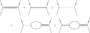
Figure 2: A diagrammatic representation of the propagator $D_{\Phi}$. The propagator, which corresponds to the curly line in the figure, describes the effective interaction between two electrons.

Within the RPA, the effective phonon action can be obtained exactly by integrating out the Hubbard-Stratonovic field $\phi$:

$$iS_{K}^{eff}[u_{cl},u_{q}]\\ =2i\int\frac{d^{2}{\bf q}}{(2\pi)^{2}}\int\frac{d\Omega}{2\pi}\vec{u}^{T*}(Q)\hat{D}^{-1}(Q)\vec{u}(Q),$$ (22)

where

$$\vec{u}^{T}(Q)=\left({\begin{array}[]{cc}u_{cl}(Q)&u_{q}(Q)\end{array}}\right).$$ (23)

As shown in the Appendix A, the inverse phonon propagator matrix $\hat{D}^{-1}$ possesses the bosonic causality structure in Keldysh space. Its components are given by

$$D_{R}^{-1}(Q,V)=2\left[{D_{0R}^{-1}(Q)-\frac{|g_{{\bf q}}|^{2}\Pi_{R}(Q,V)}{\epsilon(Q,V)}}\right],$$ (24)

$$[\hat{D}^{-1}(Q,V)]^{K}\\ =2\left[{[\hat{D}_{0}^{-1}(Q)]^{K}-\frac{\left|{g_{\bf q}}\right|^{2}\Pi^{K}(Q,V)}{\epsilon(Q,V)}}\right].$$ (25)

where the nonequilibrium polarization functions are given by

$$\Pi^{R}(K,V)=\frac{-i}{2}\int_{Q}\left[G^{K}(K+Q)G^{A}(Q)\right.\\ \left.+G^{R}(K+Q)G^{K}(Q)\right]=\Pi^{A*}(K,V)$$ (26)

$$\Pi^{K}(K,V)=\frac{-i}{2}\int_{Q}\left[G^{K}(K+Q)G^{K}(Q)\right.\\ \left.+G^{R}(K+Q)G^{A}(Q)+G^{A}(K+Q)G^{R}(Q)\right].$$ (27)

Here, $\int_{Q}=\int d^{2}{\bf q}d\Omega/(2\pi)^{3}$. Voltage $V$ is defined by $V=\mu_{L}-\mu_{R}$. $\epsilon(Q,V)$ denotes the nonequilibrium dielectric function which is defined by

$$\epsilon(Q,V)=1-V^{ee}_{{\bf q}}\Pi_{R}(Q,V).$$ (28)

We see in Eqs.24,25 that the voltage dependence of nonequilibrium phonon propagators is encoded in the self-energy part; this is consistent with the fact that phonons are driven out of equilibrium only through its coupling to the electrons. The Keldysh phonon propagators (Eqs.24,25) and the nonequilibrium polarization bubbles (Eqs.26,27) will now be used to calculate various properties of our nonequilibrium electron-phonon system. In particular, we compute the effects of voltage on the phonon velocity, electron-phonon scattering rate and electron mass enhancement, and compare the results with the corresponding results in thermal equilibrium.

III Properties of the Nonequilibrium Electron-Phonon System

III.1 Preliminary Considerations

There are four energy scales in our system: temperature/voltage $T/V$, the Debye frequency $\omega_{D}$, the layer-lead scattering rate $\Gamma$ and the average Fermi energy of the two leads $\mu$. Clearly, the mass difference between ions and electrons lead to a large discrepancy between the dynamic time scales of these species, i.e. $\omega_{D}\ll\mu$. Due to this difference, we are justified to employ the adiabatic approximation for the electrons in which we assume that electrons take on the configurations they would have if the ions were frozen into their instantaneous positions. In this approximation, a frequency-independent (static) dielectric function can be used.

We assume that the layer-lead scattering rate satisfies $\omega_{D}\ll\Gamma\ll\mu$. Working in this limit validates an expansion with respect to parameter, $\Omega/\Gamma\ll 1$, where $\Omega$ is the typical energy scale of the excitations. The limit is consistent with the necessity of a strong layer-lead coupling in order for electrons to remain out of equilibrium midst other thermalizing effects within the layer. In all of our calculations, we assume $\mbox{max}\{T,V\}$ to be small compared to all other energy scales, or more precisely, $\mbox{max}\{T,V\}\ll\omega_{D}$. Another observation one can make is our use of a jellium model for the ions. This sets a natural cutoff in momentum at $1/a\sim q_{F}$, where $a$ is the lattice constant, because any details corresponding to length scale $a$ or less is washed away by this continuum treatment of the lattice.

In the long-wavelength ($q\ll k_{F}$), small-frequency ($\Omega\ll\Gamma$) limit, and for small voltages ($V\ll\Gamma$), the polarization functions Eqs.26,27 are given by

$$\Pi^{R}({\bf q},\Omega)\approx-c_{1}(V)+c_{2}(V)\left({\frac{q}{k_{F}}}\right)^{2}-ic_{3}(V)\frac{\Omega}{\Gamma},$$ (29)

$$\Pi^{K}({\bf q},\Omega)\approx-ic_{4}\sum_{\alpha,\beta}\frac{\Gamma_{\alpha}\Gamma_{\beta}}{\Gamma^{2}}\\ \times\coth\left({\frac{\Omega+\mu_{\alpha}-\mu_{\beta}}{2T}}\right)\frac{\Omega+\mu_{\alpha}-\mu_{\beta}}{\Gamma}.$$ (30)

Here, $\mu\equiv\left({\mu_{L}+\mu_{R}}\right)/2$ is the average chemical potential of the two leads. All coefficients ($c_{1}(V)$, $c_{2}(V)$, $c_{3}(V)$, and $c_{4}$) are positive, real, and satisfies $c_{1}(V)\sim c_{3}(V)\sim c_{4}\sim\nu\gg c_{2}(V)$. $D(\mu)$ is the density of states at $\mu$ in the presence of leads, and is given by

$$D(\mu)=\frac{\nu}{\pi}\left[{\frac{\pi}{2}+\tan^{-1}\left({\frac{\mu}{\Gamma}}\right)}\right].$$ (31)

III.2 Nonequilibrium Bohm-Staver Relation

An explicit expression for the dressed retarded phonon propagator calculated in Eq.24 is

$$D_{R}(Q)=\frac{\omega_{p}}{\Omega^{2}-\omega_{p}^{2}-\frac{2\omega_{p}|g_{{\bf q}}|^{2}\Pi_{R}(Q,V)}{\epsilon(Q,V)}},$$ (32)

which in the long-wavelength, static limit is reduced to

$$D_{R}(Q)=\frac{\omega_{p}}{\Omega^{2}+\frac{q\omega_{p}^{2}}{2\pi e^{2}\Pi_{R}(Q=0,V)}}.$$ (33)

The pole of this propagator gives the dispersion of the non-attenuating longitudinal acoustic phonon mode,

$$\Omega_{{\bf q}}^{2}=c^{2}(V)q^{2},$$ (34)

where the voltage-dependent phonon velocity is,

$$c^{2}(V)=-\frac{Z^{2}n_{i}}{M\Pi_{R}({\bf 0},0,V)}.$$ (35)

At zero temperature, the static, long-wavelength polarization function as a function of voltage is

$$\Pi_{R}({\bf 0},0,V)=-\sum_{\alpha}\frac{\Gamma_{\alpha}}{\Gamma}D(\mu_{\alpha})\\ =-D(\mu)\left[{1-\frac{\nu}{2\pi D(\mu)}\frac{1}{1+{\mu^{2}\over\Gamma^{2}}}\frac{\Delta\Gamma}{\Gamma}{V\over\Gamma}+O\left({{V^{2}\over\Gamma^{2}}}\right)}\right],$$ (36)

where $\Delta\Gamma=\Gamma_{L}-\Gamma_{R}$. From Eqs.35,36, the nonequilibrium phonon velocity is given by

$$c^{2}(V)\approx c_{0}^{2}\left[{1+\frac{\nu}{2\pi D(\mu)}\frac{1}{1+{\mu^{2}\over\Gamma^{2}}}\frac{\Delta\Gamma}{\Gamma}{V\over\Gamma}}\right],$$ (37)

where

$$c_{0}^{2}\equiv\frac{Z^{2}n_{i}}{MD(\mu)}$$ (38)

is the equilibrium phonon velocity as obtained by Bohm and Staverbohmstaver . We notice in Eq.37 that the acoustic phonon velocity can be tuned by voltage. In particular, depending on the tunneling asymmetry and polarity, the change in the velocity with respect to its equilibrium value may be positive or negative.

The equilibrium phonon velocity Eq.38 may not be in the most familiar form. A more common form of the equilibrium phonon velocity is derived from requiring charge neutrality $n_{e}=Zn_{i}$ and the relationship of ratio $n_{e}/D(\mu)$ to the Fermi energy. In the considered nonequilibrium system such relations do not hold due to charge accumulation and an absence of a well-defined Fermi energy in the metal layer. However, Eqs.35,38 suggest that both equilibrium and nonequilibrium phonon velocities have the form of Eq.38 where nonequilibrium effects are encoded in the generalized density of states, $-\Pi_{R}({\bf 0},0,V)$. In equilibrium, the density of states is evaluated at one single chemical potential $\mu$ which is located at the Fermi distribution edge. At finite voltage, the electron distribution function can be shown to have a split-step shape

$$f^{neq}(\omega)=xf^{0}(\omega-\mu_{L})+(1-x)f^{0}(\omega-\mu_{R}),$$ (39)

Figure 3: Nonequilibrium steady-state electron distribution function for our system with $\mu_{L}-\mu_{R}=V>0$ and $x=\Gamma_{L}/\Gamma$ is shown above in bold (in the absence of electron-phonon interaction effects). The Dirac-Fermi distribution function is represented with a thin line.

where $f^{0}$ denotes the Dirac-Fermi distribution and $x=\Gamma_{L}/\Gamma$. The nonequilibrium analog of the density of states at Fermi energy is the sum of density of states at $\mu_{L}$ and $\mu_{R}$ weighted by the respective lead-layer coupling strengths, and is given by:

$$-\Pi_{R}({\bf 0},0,V)=xD(\mu_{L})+(1-x)D(\mu_{R}).$$ (40)

This voltage dependence in $-\Pi_{R}({\bf 0},0,V)$ is the origin of the voltage dependence seen in the nonequilibrium phonon velocity.

III.3 DC Electron-Phonon Scattering Rate

Here, we discuss the electron scattering rate due to longitudinal acoustic phonons. In equilibrium, at temperatures well below the Debye temperature, phonon wavevectors are of order $T/c_{0}$ or less. Then, within the wavevector space of phonons that are permitted to be absorbed or emitted by conservation laws, only a subspace of linear dimensions proportional to $T$ can actually participate. In two spatial dimensions, this subspace is one dimensional so the phase space of allowed wavevectors is proportional to $T$. Combining this with the fact that the screened electron-phonon coupling $|g_{sc}|^{2}\sim q\sim T$, we expect the electron-phonon scattering rate to decline as $1/\tau_{el-ph}\sim T^{2}$. This is what is expected in a closed system. In the considered open system, electrons can scatter into one of the leads frequently so that the chance of an electron encountering a phonon and scattering with it is decreased. Therefore, we expect a further decline in the electron-phonon scattering rate. We then extend our calculations to the zero-temperature finite voltage case where the scaling behaviour of the scattering rate with respect to voltage is determined. It is crucial to note that the behaviour of phonons depends most heavily on the nonequilibrium distribution function of the electrons. In this respect, the $T=0$, $V\neq 0$ situation is similar to the $T\neq 0$, $V=0$ situation in that the latter involves a smearing of the step distribution while the former results in a split-step distribution as shown in Fig.3. Therefore, phonons are subject to electrons whose distribution behaves similarly in both situations, and one may intuitively predict the scaling behaviours of the electron-phonon scattering rate with respect to $T$ and $V$ to be similar. We now quantify this possible similarity.

The starting point of this calculation is the one-loop self energy of the electron (Fig.4).

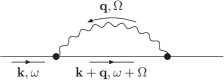
Figure 4: One-phonon self energy of the electron.

We may invoke the Migdal theorem and ignore vertex corrections. Formally, the self-energy in Fig.4 is given by

$$\Sigma^{R}(K)=2i\int_{Q}\frac{\left|{g({\bf q})}\right|^{2}}{\left|{\epsilon(Q,V)}\right|^{2}}\left(G^{R}(K+Q)D^{K}(Q)\right.\\ \left.+G^{K}(K+Q)D^{R}(Q)\right).$$ (41)

In the static, long-wavelength ($q\ll k_{F}$) limit the dielectric function is purely real and is given by

$$\epsilon_{q}(V)=\frac{2\pi e^{2}c_{1}(V)}{q}\equiv\frac{k_{S}(V)}{q},$$ (42)

where $k_{S}(V)\equiv 2\pi e^{2}c_{1}(V)$ is the 2D nonequilibrium analog of the Thomas-Fermi wavevector. At $V=0$, $c_{1}$ reduces to $D(\mu)$ and the 2D equilibrium expression for the Thomas-Fermi wavevector, $k_{S}^{0}=2\pi e^{2}D(\mu)$, is recovered. We notice that the voltage dependence observed in the Thomas-Fermi wavevector indicates that voltage can control the effectiveness of conduction electrons in screening Coulomb interactions between ions. Using $\Pi^{K}$ in the static approximation,

$$\Pi^{K}(Q,V)\\ \approx-ic_{4}\sum_{\alpha,\beta}\frac{\Gamma_{\alpha}\Gamma_{\beta}}{\Gamma^{2}}\coth\left({\frac{\Omega+\mu_{\alpha}-\mu_{\beta}}{2T}}\right)\frac{\mu_{\alpha}-\mu_{\beta}}{\Gamma},$$ (43)

the dressed phonon Green functions in the static limit can be computed as follows:

$$D^{R}(Q)={\omega_{p}\over\omega_{q}(V)}\frac{\omega_{q}(V)}{\Omega^{2}-\omega_{q}(V)^{2}+isgn(\Omega)\delta}$$ (44)

and

$$D^{K}(Q) = -\frac{[D^{-1}(Q)]^{K}}{[D^{R}(Q)]^{-1}[D^{A}(Q)]^{-1}}$$ (45)

$$= 2\left[2i\coth\left({\frac{\Omega}{2T}}\right)Im{[D_{0}^{R}(Q)]^{-1}}-\frac{\left|{g_{\bf q}}\right|^{2}\Pi^{K}(Q,V)}{\left|{\epsilon(Q,V)}\right|^{2}}\frac{ImD^{R}(Q)}{Im[D^{R}(Q)]^{-1}}\right]$$

$$= -\pi i\coth\left({\frac{\Omega}{2T}}\right)\frac{\omega_{p}}{\omega_{q}(V)}\left({\delta(\Omega-\omega_{q}(V))-\delta(\Omega+\omega_{q}(V))}\right)$$

$$\qquad\qquad+\frac{\omega_{p}}{\omega_{q}(V)}\frac{-2ic_{4}\omega_{p}\omega_{q}(V)\left|{g_{\bf q}}\right|^{2}\sum_{\alpha,\beta}\frac{\Gamma_{\alpha}\Gamma_{\beta}}{\Gamma^{2}}\coth\left({\frac{\Omega+\mu_{\alpha}-\mu_{\beta}}{2T}}\right)\frac{\mu_{\alpha}-\mu_{\beta}}{\Gamma}}{\epsilon_{q}^{2}(V)\left|{\Omega^{2}-\omega_{q}(V)^{2}+isgn(\Omega)\delta}\right|^{2}}.$$

In equilibrium, $\Pi^{K}=0$. In this case, by comparing the first term of Eq.45 with Eq.44, we can easily verify that the fluctuation dissipation theorem is satisfied.

Now one can use Eq.41 and the relevant Green functions to calculate the general DC scattering rate valid both in and out of equilibrium. Defining the static screened electron-phonon coupling constant as

$$\left|{g_{sc}({\bf q},V)}\right|^{2}\equiv\frac{\left|{g_{\bf q}}\right|^{2}\omega_{p}}{\epsilon_{q}^{2}(V)\omega_{q}(V)},$$ (46)

we obtain

$$\Sigma^{R}({\bf k}={\bf k_{F}},\omega=\mu,T,V)=\Sigma^{R}(T,V)\\ =\Sigma^{R}_{1}(T,V)+\Sigma^{R}_{2}(T,V),$$ (47)

where

$$\Sigma_{1}^{R}(T,V) = 2i\int\frac{d^{2}{\bf q}}{(2\pi)^{2}}\frac{d\Omega}{2\pi}\left|{g_{sc}({\bf q},V)}\right|^{2}\frac{1}{\Omega-v_{F}q\cos\theta+i\Gamma}\left[-\pi i\coth\left({\frac{\Omega}{2T}}\right)\left({\delta(\Omega-\omega_{q}(V))-\delta(\Omega+\omega_{q}(V))}\right)\right.$$ (48)

$$+ \left.\frac{-2ic_{4}\omega_{p}\omega_{q}(V)\left|{g_{\bf q}}\right|^{2}\sum_{\alpha,\beta}\frac{\Gamma_{\alpha}\Gamma_{\beta}}{\Gamma^{2}}\coth\left({\frac{\Omega+\mu_{\alpha}-\mu_{\beta}}{2T}}\right)\frac{\mu_{\alpha}-\mu_{\beta}}{\Gamma}}{\epsilon_{q}^{2}(V)\left|{\Omega^{2}-\omega_{q}(V)^{2}+isgn(\Omega)\delta}\right|^{2}}\right],$$

and

$$\Sigma_{2}^{R}(T,V)=2i\int\frac{d^{2}{\bf q}}{(2\pi)^{2}}\frac{d\Omega}{2\pi}\left|{g_{sc}({\bf q},V)}\right|^{2}\frac{-2i\sum_{\alpha}\Gamma_{\alpha}\tanh\left({\frac{\Omega-V_{\alpha}/2}{2T}}\right)}{\left({\Omega-v_{F}q\cos\theta}\right)^{2}+\Gamma^{2}}\frac{\omega_{q}(V)}{\Omega^{2}-\omega_{q}(V)^{2}+isgn(\Omega)\delta}.$$ (49)

Here, we have linearized the Fermion dispersion and $V_{L,R}=\pm V$ where $V=\mu_{L}-\mu_{R}\geq 0$ is assumed. Eqs.48,49 are the central results in the remaining sections of our work. In equilibrium (i.e. $\mu_{L}=\mu_{R}$), Eqs.48,49 reduce to

$$\Sigma_{1}^{R}(T)=\int\frac{qdqd\theta}{(2\pi)^{2}}d\Omega\left|{g_{sc}({\bf q})}\right|^{2}\frac{\coth\left({\frac{\Omega}{2T}}\right)\left[{\delta(\Omega-\omega_{q})-\delta(\Omega+\omega_{q})}\right]}{\left({\Omega-v_{F}q\cos\theta+i\Gamma}\right)},$$ (50)

and

$$\Sigma_{2}^{R}(T)=4\Gamma\int\frac{qdqd\theta}{(2\pi)^{2}}\frac{d\Omega}{2\pi}\left|{g_{sc}({\bf q})}\right|^{2}\frac{\tanh\left({\frac{\Omega}{2T}}\right)}{\left({\Omega-v_{F}q\cos\theta}\right)^{2}+\Gamma^{2}}\frac{\omega_{q}}{\Omega^{2}-\omega_{q}^{2}+isgn(\Omega)\delta}.$$ (51)

In the presence of voltage (at zero temperature),

$$\Sigma_{1}^{R}(V) = 2\int\frac{d^{2}{\bf q}}{(2\pi)^{2}}\frac{d\Omega}{2\pi}\left|{g_{sc}({\bf q},V)}\right|^{2}\frac{1}{\Omega-v_{F}q\cos\theta+i\Gamma}\left[\pi sgn(\Omega)\left({\delta(\Omega-\omega_{q}(V))-\delta(\Omega+\omega_{q}(V))}\right)\right.$$ (52)

$$+ \left.\frac{2c_{4}\omega_{p}\omega_{q}(V)\left|{g_{\bf q}}\right|^{2}\frac{\Gamma_{L}\Gamma_{R}V}{\Gamma^{3}}\left({sgn(\Omega+V)-sgn(\Omega-V)}\right)}{\epsilon_{q}^{2}(V)\left|{\Omega^{2}-\omega_{q}(V)^{2}+isgn(\Omega)\delta}\right|^{2}}\right],$$

and

$$\Sigma_{2}^{R}(V)=4\int\frac{d^{2}{\bf q}}{(2\pi)^{2}}\frac{d\Omega}{2\pi}\left|{g_{sc}({\bf q},V)}\right|^{2}\frac{\sum_{\alpha}\Gamma_{\alpha}sgn\left({\Omega-V_{\alpha}/2}\right)}{\left({\Omega-v_{F}q\cos\theta}\right)^{2}+\Gamma^{2}}\frac{\omega_{q}(V)}{\Omega^{2}-\omega_{q}(V)^{2}+isgn(\Omega)\delta}.$$ (53)

III.3.1 Thermal Equilibrium: $T\neq 0$, $V=0$

In equilibrium scattering rate calculations, temperature $T$ defines a natural cutoff for the momentum integrals. This is because only phonons of frequencies comparable or less than $T$ can be absorbed or emitted. For $T\ll\omega_{D}$, the phonon dispersion obeys $\omega_{q}=c_{0}q$ which implies that phonon wavevectors are of order $T/c_{0}$ or less. We now proceed with the integrals in Eqs.50,51. The angular integration can be done straightforwardly. For $\frac{\omega+\Omega}{\Gamma}\ll 1$,

$$\int_{0}^{2\pi}\frac{d\theta}{2\pi}\frac{1}{\omega+\Omega-v_{F}q\cos\theta+i\Gamma}\\ \approx-if_{0}(q)+f_{1}(q)\frac{\omega+\Omega}{\Gamma},$$ (54)

where

$$f_{0}(q)=\frac{1}{\Gamma}\frac{1}{\left[{1+\left({\frac{v_{F}q}{\Gamma}}\right)^{2}}\right]^{1/2}},$$ (55)

$$f_{1}(q)=\frac{1}{\Gamma}\frac{1}{\left[{1+\left({\frac{v_{F}q}{\Gamma}}\right)^{2}}\right]^{3/2}}.$$ (56)

Using this result one obtains,

$$-Im\Sigma^{R}_{1}(T) \approx \frac{2}{\Gamma}\int_{0}^{T/c_{0}}\frac{qdq}{2\pi}\left|{g_{sc}({\bf q})}\right|^{2}\coth\left({\frac{c_{0}q}{2T}}\right)$$ (57)

$$= \frac{GT^{3}}{\Gamma c_{0}^{3}}\underbrace{2\int_{0}^{1}\frac{y^{2}dy}{2\pi}\coth\left({\frac{y}{2}}\right)}_{\gamma^{eq}_{1}}$$

$$= \frac{G\gamma^{eq}_{1}}{\Gamma c_{0}^{3}}T^{3},$$

where $\gamma^{eq}_{1}\sim O(1)$ and

$$G(V)=\frac{\left|{g_{sc}({\bf q},V)}\right|^{2}}{q}$$ (58)

is a real quantity independent of $Q$. We have also used the fact that in the region of $q$ over which the integral is conducted, the dielectric function and $f_{0}$ can be approximated by

$$\epsilon(q)\approx\frac{k_{S}^{0}}{q}\qquad\qquad f_{0}(q)\approx\frac{1}{\Gamma}.$$ (59)

Similarly, we get

$$-Im\Sigma^{R}_{2}(T) \approx \frac{1}{\Gamma}\int_{0}^{T/c_{0}}\frac{qdq}{2\pi}\left|{g_{sc}({\bf q})}\right|^{2}\tanh\left({\frac{c_{0}q}{2T}}\right)$$ (60)

$$= \frac{GT^{3}}{\Gamma c_{0}^{3}}\underbrace{\int_{0}^{1}\frac{y^{2}dy}{2\pi}\tanh\left({\frac{y}{2}}\right)}_{\gamma^{eq}_{2}}$$

$$= \frac{G\gamma^{eq}_{2}}{\Gamma c_{0}^{3}}T^{3},$$

where $\gamma^{eq}_{2}\sim O(1)$. Therefore, in thermal equilibrium,

$${1\over\tau_{el-ph}^{eq}}=\frac{G\gamma^{eq}}{\Gamma c_{0}^{3}}T^{3},$$ (61)

where $\gamma^{eq}\sim O(1)$.

III.3.2 Out of Equilibrium: $V\neq 0$, $T=0$

In the nonequilibrium case, the momentum cutoff is set by the voltage, i.e. $q_{c}\sim V/c(V)$. Therefore, the DC scattering rate is at least of order $V$, and thus, we may set $V=0$ for the quantities in the integrand such as the phonon velocity and dielectric function. This should allow us to obtain the scattering rate to leading order in $V$. When the first integral Eq.52 is naïvely evaluated we find that the second term, which becomes finite out of equilibrium, gives a divergent contribution to the scattering rate. This divergence can be cured by dropping the static limit assumption and expanding the dielectric function to lowest order in frequency,

$$\epsilon(Q)\approx 1+c_{1}\frac{2\pi e^{2}}{q}+ic_{3}\frac{2\pi e^{2}}{q}\frac{\Omega}{\Gamma}.$$ (62)

Recall that for $\mu\gg\Gamma$,

$$c_{1}\approx c_{4}\approx 2c_{3}\approx\nu.$$ (63)

Therefore, we get

$$\epsilon(Q)\approx\frac{k_{S}^{0}}{q}\left({1+i\frac{\Omega}{2\Gamma}}\right),$$ (64)

where $k_{S}^{0}\equiv 2\pi e^{2}\nu$. This new expression for the dielectric function assumes that typical excitation energy scale is smaller than $\Gamma$. The phonon dispersion then becomes dissipative:

$$\tilde{\omega}_{q}^{2}=\frac{\omega_{p}^{2}(q)}{\epsilon(Q,V)}\approx\omega_{q}^{2}\left({1-i\frac{\Omega}{2\Gamma}}\right),$$ (65)

where $\omega_{q}$ is phonon dispersion in the static limit. The modified phonon Green functions are,

$$D^{R}(Q)=\frac{\omega_{p}}{\Omega^{2}-\omega_{q}^{2}(V)+i\omega_{q}^{2}(V)\frac{\Omega}{2\Gamma}},$$ (66)

$$D^{K}(Q)=\frac{2\left|{g_{\bf q}}\right|^{2}\Pi^{K}(Q,V)}{\left|{\epsilon_{q}(\Omega,V)}\right|^{2}\omega_{q}^{4}(V)}\frac{\omega_{p}^{2}}{\left({1-\frac{\Omega^{2}}{\omega_{q}^{2}(V)}}\right)^{2}+\frac{\Omega^{2}}{4\Gamma^{2}}}.$$ (67)

Now we are set to compute the first self-energy term,

$$-Im\Sigma_{1}^{R}(V)=4\int\frac{qdq}{2\pi}\frac{d\Omega}{2\pi}\left|{g_{sc}({\bf q})}\right|^{4}f_{0}(q)\frac{-Im\Pi^{K}(Q)}{\omega_{q}^{2}\left({1+\frac{\Omega^{2}}{4\Gamma^{2}}}\right)^{2}}\frac{1}{\left({1-\frac{\Omega^{2}}{\omega_{q}^{2}}}\right)^{2}+\frac{\Omega^{2}}{4\Gamma^{2}}}.$$ (68)

We see that majority of the contribution in the integral comes from $\Omega\sim\omega_{q}$. So one may cutoff the $\Omega$-integral by $V\ll\Gamma$. If we cutoff $q$ at $q_{c}\sim\frac{V}{c_{0}}$, $\Omega_{c}\sim V\ll\Gamma$. The static expression for the Keldysh polarization function must be made consistent with the approximate dynamic dielectric function. For $\Omega\leq V$,

$$-Im\Pi^{K}(Q)\approx D_{0}\left[{\frac{\Gamma_{L}^{2}+\Gamma_{R}^{2}}{\Gamma^{3}}\left|{\Omega}\right|+\frac{2\Gamma_{L}\Gamma_{R}}{\Gamma^{3}}V}\right].$$ (69)

After a series of integrals, we get

$$-Im\Sigma_{1}^{R}(V)=\frac{G^{2}D_{0}\gamma^{neq}_{1}}{\Gamma^{2}c_{0}^{4}}\left[{1+\frac{2\Gamma_{L}\Gamma_{R}}{\Gamma^{2}}}\right]V^{4},$$ (70)

where $\gamma^{neq}_{1}\sim O(1)$. This gives us a fourth order contribution and will become a subdominant correction to the second integral as we will now show. The second integral from Eq.53 can be done straightforwardly:

$$-Im\Sigma^{R}_{2}(V) \approx \frac{1}{\Gamma^{2}}\int_{0}^{V/c_{0}}\frac{qdq}{2\pi}\left|{g_{sc}({\bf q})}\right|^{2}\Gamma$$ (71)

$$\times \left({sgn(\omega_{q}-V/2)+sgn(\omega_{q}+V/2)}\right)$$

$$= \frac{GV^{3}}{\Gamma c_{0}^{3}}\underbrace{\int_{1/2}^{1}\frac{y^{2}dy}{2\pi}}_{\gamma^{neq}_{2}}$$

$$= \frac{G\gamma^{neq}_{2}}{\Gamma c_{0}^{3}}V^{3},$$

where $\gamma^{neq}_{2}\sim O(1)$. Therefore, to lowest order in voltage we obtain,

$${1\over\tau_{el-ph}^{neq}}\approx\frac{G\gamma^{neq}}{\Gamma c_{0}^{3}}V^{3},$$ (72)

where $\gamma^{neq}\sim O(1)$.

We can summarize the low-$T$/low-$V$ electron-phonon scattering rate both in and out of equilibrium:

$${1\over\tau_{el-ph}} = \frac{G\gamma_{X}}{\Gamma c_{0}^{3}}X^{3}$$ (75)

where $$\left\{\begin{array}[]{r@{\quad:\quad}l}X=T&T\neq 0,V=0\\ X=\left|{V}\right|&T=0,V\neq 0\end{array}\right.,$$

where $\gamma_{X}$ is some real constant of $O(1)$.

III.4 Electron Mass Enhancement

We now compute the effective on-shell mass correction and investigate the effects of temperature and voltage to lowest order.

III.4.1 Thermal Equilibrium $T\neq 0$, $V=0$

From Eqs.50,51 we obtain,

$$Re\Sigma_{1}^{R}(\omega,T)\\ =2\int\frac{qdq}{2\pi}\left|{g_{sc}({\bf q})}\right|^{2}\coth\left({\frac{\omega_{q}}{2T}}\right)f_{1}(q)\frac{\omega}{\Gamma},$$ (76)

$$Re\Sigma_{2}^{R}(\omega,T)=2\int\frac{qdq}{2\pi}\int\frac{d\Omega}{2\pi}\left|{g_{sc}({\bf q})}\right|^{2}\\ \times\tanh\left({\frac{\omega+\Omega}{2T}}\right)f_{0}(q)P\left({\frac{2\omega_{q}}{\Omega^{2}-\omega_{q}^{2}}}\right).$$ (77)

It is useful to separate out the zero and finite temperature contributions to the mass enhancement by defining

$$\lambda_{i}(T)=\lambda_{i}^{0}+\delta\lambda_{i}(T),$$ (78)

where

$$\lambda_{i}^{0}\equiv-\left.\frac{\partial Re\Sigma_{i}^{R}(\omega,T=0)}{\partial\omega}\right|_{\omega=0},$$ (79)

$$\delta\lambda_{i}(T)\equiv-\left[\left.\frac{\partial Re\Sigma_{i}^{R}(\omega,T)}{\partial\omega}\right|_{\omega=0}\right.\\ \left.-\left.\frac{\partial Re\Sigma_{i}^{R}(\omega,T=0)}{\partial\omega}\right|_{\omega=0}\right].$$ (80)

Here, $i\in\{1,2\}$ labels the two self-energy contributions (Eqs.76,77). The zero temperature contribution is then given by,

$$\lambda^{0}=\sum_{i=1}^{2}\lambda_{i}^{0}\\ =\frac{2G}{\pi^{2}}\int_{0}^{q_{D}\sim k_{F}}q^{2}dq\frac{f_{0}(q)}{\omega_{q}}\left({1-\frac{\pi}{2}\frac{f_{1}(q)}{f_{0}(q)}\frac{\omega_{q}}{\Gamma}}\right).$$ (81)

We see that the second term in the round brackets is much smaller than 1 for $q\leq k_{F}$. So we neglect this term and obtain the zero temperature enhanced mass in equilibrium:

$$\lambda^{0} \approx \frac{2G}{\pi^{2}c_{0}^{2}}\int_{0}^{k_{F}}qdqf_{0}(q)$$ (82)

$$= \frac{2G\mu}{\pi^{2}c_{0}v_{F}^{2}}.\qquad(\mu\gg\Gamma)$$

At finite temperature, the effective mass correction gains a temperature correction. The first correction is given by,

$$\delta\lambda_{1}(T)=-\frac{2G}{\Gamma}\int\frac{q^{2}dq}{2\pi}\left[{\coth\left({\frac{\omega_{q}}{2T}}\right)-1}\right]f_{1}(q).$$ (83)

We see that the integrand is negligibly small for $q\geq\alpha\frac{T}{c_{0}}$ where $\alpha\sim O(1)$. Then, employing this momentum cutoff we get,

$$\delta\lambda_{1}(T) = -\frac{2G}{\Gamma}\int_{0}^{\alpha\frac{T}{c_{0}}}\frac{q^{2}dq}{2\pi}\left[{\coth\left({\frac{c_{0}q}{2T}}\right)-1}\right]f_{1}(q)$$ (84)

$$\approx -\frac{G}{\Gamma^{2}}\left({\frac{T}{c_{0}}}\right)^{3}\underbrace{\frac{1}{\pi}\int_{0}^{\alpha}y^{2}dy\left[{\coth\left({\frac{y}{2}}\right)-1}\right]}_{l_{3}}$$

$$= -\frac{G}{c_{0}^{3}\Gamma^{2}}l_{3}T^{3},$$

where $l_{3}>0$ is a constant of $O(1)$. The second contribution is,

$$\delta\lambda_{2}(T)=-2\int\frac{qdq}{2\pi}\frac{d\Omega}{2\pi}\left|{g_{sc}(q)}\right|^{2}f_{0}(q)\\ \times\left({\frac{1}{2T}\mbox{sech}^{2}\left({\frac{\Omega}{2T}}\right)-2\delta(\Omega)}\right)P\left({\frac{2\omega_{q}}{\Omega^{2}-\omega_{q}^{2}}}\right).$$ (85)

We see that the integrand is negligibly small for phonon frequencies $\Omega\geq\alpha T$ where once again $\alpha\sim O(1)$. In the second term, this corresponds to a momentum cutoff of $q_{c}=\alpha\frac{T}{c_{0}}$. Applying these cutoffs we obtain the second correction

$$\delta\lambda_{2}(T)=\frac{G}{c_{0}^{3}\Gamma}l_{2}T^{2},$$ (86)

where the constant $l_{2}\sim O(1)>0$ is given by

$$l_{2}=\frac{1}{2\pi^{2}}\int_{-\alpha}^{\alpha}dx\mbox{sech}^{2}\left({\frac{x}{2}}\right)\\ \times\left({\alpha^{2}+x^{2}\ln\left|{\frac{\alpha^{2}}{x^{2}}-1}\right|}\right)-\frac{\alpha^{2}}{\pi^{2}}.$$ (87)

In conclusion, the electron mass enhancement at thermal equilibrium to lowest order in temperature is

$$\lambda(T)=\frac{2G\mu}{\pi^{2}c_{0}v_{F}^{2}}+\frac{G\Gamma}{c_{0}^{3}}l_{2}\left({\frac{T}{\Gamma}}\right)^{2}.$$ (88)

III.4.2 Out of Equilibrium $T=0$, $V\neq 0$

We begin the nonequilibrium calculation with the second contribution $\Sigma_{2}^{R}(\omega,V)$,

$$Re\Sigma_{2}^{R}(\omega,V)=2\sum_{\alpha}\frac{\Gamma_{\alpha}}{\Gamma}\int\frac{qdq}{2\pi}\frac{d\Omega}{2\pi}\left|{g_{sc}({\bf q})}\right|^{2}\\ \times sgn\left({\omega+\Omega-\frac{V_{\alpha}}{2}}\right)f_{0}(q)P\left({\frac{2\omega_{q}}{\Omega^{2}-\omega_{q}^{2}}}\right).$$ (89)

Then the finite voltage correction is given by

$$\delta\lambda_{2}(V) = 4G\int\frac{q^{2}dq}{2\pi}\frac{d\Omega}{2\pi}f_{0}(q)P\frac{2\omega_{q}}{\Omega^{2}-\omega_{q}^{2}}$$ (90)

$$\times \left[{\delta\left({\Omega}\right)-\sum_{\alpha}\frac{\Gamma_{\alpha}}{\Gamma}\delta\left({\frac{V_{\alpha}}{2}-\Omega}\right)}\right]$$

$$= \frac{G}{\Gamma c_{0}^{3}}V^{2}\underbrace{\left[{\frac{1}{\pi^{2}}P\int_{0}^{1}dy\frac{4y}{4y^{2}-1}}\right]}_{k_{2}}$$

$$= \frac{G\Gamma}{c_{0}^{3}}k_{2}\left({\frac{V}{\Gamma}}\right)^{2}.$$

Here, $k_{2}\sim O(1)$ is a positive constant. For the calculation of $\delta\lambda_{1}(V)$ one needs to go beyond the static approximation for the dielectric function as was done for the scattering rate calculation. Thus, the correction to the effective mass parameter from the first contribution is given by

$$\delta\lambda_{1}(V) = -\frac{D_{0}}{\pi^{2}\Gamma}\frac{2\Gamma_{L}\Gamma_{R}V}{\Gamma^{3}}$$ (91)

$$\times \int qdqd\Omega f_{1}(q)\frac{\left|{g_{q}}\right|^{4}\omega_{p}^{2}}{\omega_{q}^{4}}\frac{q^{4}}{k_{S}^{4}}\frac{1}{\left({1-\frac{\Omega^{2}}{\omega_{q}^{2}}}\right)^{2}+\frac{\Omega^{2}}{4\Gamma^{2}}}$$

$$\approx -\frac{D_{0}}{\pi^{2}\Gamma}\frac{2\Gamma_{L}\Gamma_{R}}{\Gamma^{2}}\left({\frac{V}{\Gamma}}\right)^{2}\int_{0}^{V/c_{0}}qdq\frac{G^{2}q^{2}}{c_{0}^{2}q^{2}}$$

$$= -\frac{D_{0}G^{2}\Gamma_{L}\Gamma_{R}}{\pi^{2}\Gamma c_{0}^{4}}\left({\frac{V}{\Gamma}}\right)^{4}.$$

The electron mass enhancement to lowest order in voltage is then,

$$\lambda(V)=\frac{2G\mu}{\pi^{2}c_{0}v_{F}^{2}}+\frac{G\Gamma}{c_{0}^{3}}k_{2}\left({\frac{V}{\Gamma}}\right)^{2}.$$ (92)

In conclusion, the electron mass enhancement to lowest order in $\frac{T}{\Gamma}$ or $\frac{V}{\Gamma}$, can be summarized concisely by

$$\lambda(X) = \frac{2G\mu}{\pi^{2}c_{0}v_{F}^{2}}+\frac{G\Gamma}{c_{0}^{3}}\kappa_{X}\left({\frac{X}{\Gamma}}\right)^{2}$$ (95)

where $$\left\{\begin{array}[]{r@{\quad:\quad}l}X=T&T\neq 0,V=0\\ X=V&T=0,V\neq 0\end{array}\right.,$$

where $\kappa_{X}$ is a real constant of $O(1)$.

IV Conclusion

In this paper we studied a simple model of a steady-state electrically-driven two-dimensional electron-phonon system. The drive was applied to the metallic layer by attaching two 3D leads, which acted both as a source of particles (current source) and a heat sink. The resultant current was perpendicular to the layer so that the heating problem could be avoided. The effective theory for the metallic layer was developed using the Keldysh path integral method.

We found that various properties of the electron-phonon system is modified in the presence of an out-of-plane voltage. Voltage dependences in the Thomas-Fermi screening length and in the velocity of the longitudinal acoustic phonon mode are presented. The results show that both of these quantities can be tuned at will using the external voltage. In-plane electron-phonon scattering rate and electron mass enhancement were also investigated. We showed that electron-phonon scattering can be enhanced by voltage at zero temperature. The computed modification to the electron mass enhancement by voltage implies the possibility of tuning the effective mass of the electron using voltage.

The in-plane electron-phonon scattering rate can be indirectly measured by observing the voltage-dependent piece of the in-plane resistivity, $\rho^{V}_{xx}$. The resistivity can be measured as a linear response to the in-plane current drive. Since the electron-phonon scattering rate occurs predominantly in the forward scattering channels, $\rho^{V}_{xx}$ gains an additional factor of $V^{2}$ compared to the scattering rate. Therefore, the finite voltage correction to the in-plane resistivity should scale as $\rho^{V}_{xx}\sim V^{5}$.

Renormalizations to the electron effective mass and electron distribution due to external voltage may be observed in a Shubnikov-de-Haas experiment. In the presence of a magnetic field normal to the metallic layer (${\bf B}=B\hat{{\bf z}}$), the layer electrons undergo an in-plane cyclotron motion. The electron energies are quantized according to an energy spectrum composed of Landau levels, which are separated by the cyclotron energy. The resultant electron density of states show multiple peaks, each peak corresponding to a Landau level. Because the separation between a pair of Landau levels depends linearly on magnetic field, the longitudinal in-plane resistivity oscillates as a function of the magnetic field. This oscillation is the well-known Shubnikov-de-Haas effect. The difference in the extrema of the oscillations as a function of magnetic field decays exponentially as the field is decreasedcoleridgeetal ; mancoffetal . The cyclotron frequency can be obtained by observing the characteristic energy scale with which this decay occurs. The effective electron mass, in turn, can be found by its direct relationship to the cyclotron frequency.

We also predict that the observed Shubnikov-de-Haas oscillations should contain features that specifically result from the structure of the zero-temperature nonequilibrium electron distribution. Out of equilibrium, the distribution function assumes the split-step shapecomm , in which each step is presumably of different height given the asymmetry in the lead-layer couplings. As the magnetic field is varied, both of these steps become resonant with a Landau level. As a result, each extremum in the resistivity would, in principle, split into two asymmetric peaks.

Appendix A Keldysh Action for Phonons

The purpose of this appendix is to begin with the real time action for the Hamiltonian given in section II.1 and show detailed Keldysh calculations that lead to the effective phonon action Eq.22, from which the inverse retarded, advanced and Keldysh phonon propagators can be read off directly.

Our starting real time action, after the lead electrons have been integrated out, is

$$iS[d,\bar{d},u,u^{*}]=iS_{el}[d,\bar{d}]+iS_{ph}[u,u^{*}]+iS_{el-ph}[d,\bar{d},u,u^{*}],$$ (96)

where

$$\begin{split}iS_{el}[d,\bar{d}]&=i\int dtdt^{\prime}\sum_{{\bf k},\sigma}\bar{d}_{\sigma}({\bf k},t^{\prime})G^{-1}({\bf k},t^{\prime}-t)d_{\sigma}({\bf k},t)\\ &-i\int dt\sum_{{\bf q}\neq 0}\sum_{{\bf k},{\bf k^{\prime}}\atop\sigma,\sigma^{\prime}}\frac{V^{ee}_{{\bf q}}}{2}\bar{d}_{\sigma}({\bf k+q},t)\bar{d}_{\sigma^{\prime}}({\bf k^{\prime}-q},t)d_{\sigma^{\prime}}({\bf k^{\prime}},t)d_{\sigma}({\bf k},t),\\ iS_{ph}[u,u^{*}]&=\int dtu^{*}({\bf k},t^{\prime})D_{0}^{-1}({\bf k},t^{\prime}-t)u({\bf k},t),\\ iS_{el-ph}[d,\bar{d},u,u^{*}]&=-i\int dt\sum_{{\bf k},{\bf q},\sigma}g_{{\bf q}}\bar{d}_{\sigma}({\bf k+q},t)d_{\sigma}({\bf k},t)u({\bf q},t).\end{split}$$ (97)

In order to carry out the time loop contour integration, we split all fields into two components, forward ($+$) and backward ($-$) fields, which reside on the forward and backward branches of the time loop contour, respectively. The action then can be written in the form,

$$iS^{K}[d,\bar{d},u,u^{*},\phi,\phi^{*}]=iS^{K}[d_{+},\bar{d}_{+},u_{+},u^{*}_{+},\phi_{+},\phi^{*}_{+}]-iS^{K}[d_{-},\bar{d}_{-},u_{-},u^{*}_{-},\phi_{-},\phi^{*}_{-}].$$ (98)

Here, $\phi$ is a Hubbard-Stratonovic field used to decouple the quartic term in Eq.97. In this basis for the Keldysh space (i.e. $+$,$-$ fields) one obtains four Green functions for every field, one of which can be expressed as a linear combination of the other three. Therefore, one often performs a linear transformation of the fields so as to work with three independent Green functions. This is known as Keldysh rotationkamenev ; rammer , in which new fermion fields are defined via

$$f_{1}=\frac{f_{+}+f_{-}}{2}\qquad f_{2}=\frac{f_{+}-f_{-}}{2}\qquad\bar{f}_{1}=\frac{\bar{f}_{+}-\bar{f}_{-}}{2}\qquad\bar{f}_{2}=\frac{\bar{f}_{+}+\bar{f}_{-}}{2},$$ (99)

and new boson fields are defined via

$$b_{cl}=\frac{b_{+}+b_{-}}{2}\qquad b_{q}=\frac{b_{+}-b_{-}}{2}\qquad b_{cl}^{*}=\frac{b_{+}^{*}+b_{-}^{*}}{2}\qquad b_{q}^{*}=\frac{b_{+}^{*}-b_{-}^{*}}{2}.$$ (100)

Upon carrying out the Keldysh rotation on the time loop contour action of Eq.98 we obtain,

$$\begin{split}iS^{el}_{K}&=2i\int dt\sum_{{\bf k},{\bf k^{\prime}},\sigma}\left({\begin{array}[]{cc}\bar{d}_{\sigma}^{1}({\bf k^{\prime}},t)&\bar{d}_{\sigma}^{2}({\bf k^{\prime}},t)\end{array}}\right)\left[\left({\begin{array}[]{cc}G_{R}^{-1}({\bf k},t)\delta_{{\bf k^{\prime}}{\bf k}}&[\hat{G}^{-1}]_{K}({\bf k},t)\delta_{{\bf k^{\prime}}{\bf k}}\\ 0&G_{A}^{-1}({\bf k},t)\delta_{{\bf k^{\prime}}{\bf k}}\end{array}}\right)\right.\\ &+\left.\left({\begin{array}[]{cc}e\phi^{cl}({\bf k^{\prime}}-{\bf k},t)-g_{{\bf k^{\prime}}-{\bf k}}u^{cl}({\bf k^{\prime}}-{\bf k},t)&e\phi^{q}({\bf k^{\prime}}-{\bf k},t)-g_{{\bf k^{\prime}}-{\bf k}}u^{q}({\bf k^{\prime}}-{\bf k},t)\\ e\phi^{q}({\bf k^{\prime}}-{\bf k},t)-g_{{\bf k^{\prime}}-{\bf k}}u^{q}({\bf k^{\prime}}-{\bf k},t)&e\phi^{cl}({\bf k^{\prime}}-{\bf k},t)-g_{{\bf k^{\prime}}-{\bf k}}u^{cl}({\bf k^{\prime}}-{\bf k},t)\end{array}}\right)\right]\left({\begin{array}[]{c}d_{\sigma}^{1}({\bf k},t)\\ d_{\sigma}^{2}({\bf k},t)\end{array}}\right)\\ iS^{ch}_{K}&=2i\int dt\sum_{{\bf k}}\left({\begin{array}[]{cc}\phi^{cl*}({\bf k},t)&\phi^{q*}({\bf k},t)\end{array}}\right)\left({\begin{array}[]{cc}0&\frac{k}{2\pi}\\ \frac{k}{2\pi}&0\end{array}}\right)\left({\begin{array}[]{c}\phi^{cl}({\bf k},t)\\ \phi^{q}({\bf k},t)\end{array}}\right)\\ iS^{ph}_{K}&=2i\int dt\sum_{{\bf k}}\left({\begin{array}[]{cc}u^{cl*}({\bf k},t)&u^{q*}({\bf k},t)\end{array}}\right)\left({\begin{array}[]{cc}0&[D_{0}^{A}({\bf k},t)]^{-1}\\ \left[{D_{0}^{R}({\bf k},t)}\right]^{-1}&\left[{\hat{D}_{0}^{-1}({\bf k},t)}\right]^{K}\end{array}}\right)\left({\begin{array}[]{c}u^{cl}({\bf k},t)\\ u^{q}({\bf k},t)\end{array}}\right).\end{split}$$ (101)

Integrating out the layer electrons in $iS^{el}_{K}$, we get

$$iS^{eff}_{K}[\Phi,\Phi^{*}]=-2i\sum_{{\bf k},\omega}\left({\begin{array}[]{cc}\Phi^{cl*}({\bf k},\omega)&\Phi^{q*}({\bf k},\omega)\end{array}}\right)\left({\begin{array}[]{cc}0&\Pi^{A}({\bf k},\omega)\\ \Pi^{R}({\bf k},\omega)&\Pi^{K}({\bf k},\omega)\end{array}}\right)\left({\begin{array}[]{c}\Phi^{cl}({\bf k},\omega)\\ \Phi^{q}({\bf k},\omega)\end{array}}\right).$$ (102)

When Eq.102 is expanded, the total action now becomes,

$$\begin{split}iS_{k}^{eff}[u,u^{*},\phi,\phi^{*}]&=2i\sum_{{\bf k},\omega}\left({\begin{array}[]{cc}u^{cl*}({\bf k},\omega)&u^{q*}({\bf k},\omega)\end{array}}\right)\left({\begin{array}[]{cc}0&[D_{0}^{A}({\bf k},\omega)]^{-1}\\ \left[{D_{0}^{R}({\bf k},\omega)}\right]^{-1}&\left[{D_{0}^{-1}({\bf k},\omega)}\right]^{K}\end{array}}\right)\left({\begin{array}[]{c}u^{cl}({\bf k},\omega)\\ u^{q}({\bf k},\omega)\end{array}}\right)\\ &+2i\sum_{{\bf k},\omega}\left({\begin{array}[]{cc}\phi^{cl*}({\bf k},\omega)&\phi^{q*}({\bf k},\omega)\end{array}}\right)\left({\begin{array}[]{cc}0&\frac{k}{2\pi}\\ \frac{k}{2\pi}&0\end{array}}\right)\left({\begin{array}[]{c}\phi^{cl}({\bf k},\omega)\\ \phi^{q}({\bf k},\omega)\end{array}}\right)\\ &-2ie^{2}\sum_{{\bf k},\omega}\left({\begin{array}[]{cc}\phi^{cl*}({\bf k},\omega)&\phi^{q*}({\bf k},\omega)\end{array}}\right)\left({\begin{array}[]{cc}0&\Pi^{A}({\bf k},\omega)\\ \Pi^{R}({\bf k},\omega)&\Pi^{K}({\bf k},\omega)\end{array}}\right)\left({\begin{array}[]{c}\phi^{cl}({\bf k},\omega)\\ \phi^{q}({\bf k},\omega)\end{array}}\right)\\ &+2ie\sum_{{\bf k},\omega}g^{*}_{{\bf k}}\left({\begin{array}[]{cc}u^{cl*}({\bf k},\omega)&u^{q*}({\bf k},\omega)\end{array}}\right)\left({\begin{array}[]{cc}0&\Pi^{A}({\bf k},\omega)\\ \Pi^{R}({\bf k},\omega)&\Pi^{K}({\bf k},\omega)\end{array}}\right)\left({\begin{array}[]{c}\phi^{cl}({\bf k},\omega)\\ \phi^{q}({\bf k},\omega)\end{array}}\right)\\ &+2ie\sum_{{\bf k},\omega}g_{{\bf k}}\left({\begin{array}[]{cc}\phi^{cl*}({\bf k},\omega)&\phi^{q*}({\bf k},\omega)\end{array}}\right)\left({\begin{array}[]{cc}0&\Pi^{A}({\bf k},\omega)\\ \Pi^{R}({\bf k},\omega)&\Pi^{K}({\bf k},\omega)\end{array}}\right)\left({\begin{array}[]{c}u^{cl}({\bf k},\omega)\\ u^{q}({\bf k},\omega)\end{array}}\right)\\ &-2i\sum_{{\bf k},\omega}|g_{{\bf k}}|^{2}\left({\begin{array}[]{cc}u^{cl*}({\bf k},\omega)&u^{q*}({\bf k},\omega)\end{array}}\right)\left({\begin{array}[]{cc}0&\Pi^{A}({\bf k},\omega)\\ \Pi^{R}({\bf k},\omega)&\Pi^{K}({\bf k},\omega)\end{array}}\right)\left({\begin{array}[]{c}u^{cl}({\bf k},\omega)\\ u^{q}({\bf k},\omega)\end{array}}\right).\end{split}$$ (103)

The $\Phi$ fields were defined in Eq.17 and the Keldysh polarization diagrams ($\Pi$) were defined in Eqs.26,27. Expressions for the retarded and Keldysh polarization diagrams in the long-time, long-wavelength limit were introduced in Eqs.29,30. The coefficients appearing in these approximate expressions are given by,

$$c_{1}(V) \equiv \sum_{\alpha}\frac{\Gamma_{\alpha}}{\Gamma}D(\mu_{\alpha})$$ (104)

$$c_{2}(V) \equiv \frac{D_{0}}{3\pi}\sum_{\alpha}\frac{\Gamma_{\alpha}}{\mu}\frac{\mu^{2}}{\mu_{\alpha}^{2}+\Gamma^{2}}$$ (105)

$$c_{3}(V) \equiv \sum_{\alpha}\frac{\Gamma_{\alpha}}{2\Gamma}\left[{D(\mu_{\alpha})+\frac{D_{0}}{\pi}\frac{\Gamma}{\mu_{\alpha}}\frac{1}{1+\frac{\Gamma^{2}}{\mu_{\alpha}^{2}}}}\right]$$ (106)

$$c_{4} \equiv D(\mu)+\frac{D_{0}\Gamma}{\pi\mu}\frac{1}{1+\frac{\Gamma^{2}}{\mu^{2}}}.$$ (107)

Now integrating out the $\phi$ field, we obtain

$$\begin{split}iS_{K}^{eff}[u,u^{*}]&=2i\sum_{{\bf k},\omega}\left({\begin{array}[]{cc}u^{cl*}({\bf k},\omega)&u^{q*}({\bf k},\omega)\end{array}}\right)\left({\begin{array}[]{cc}0&[D_{0}^{A}({\bf k},\omega)]^{-1}\\ \left[{D_{0}^{R}({\bf k},\omega)}\right]^{-1}&\left[{D_{0}^{-1}({\bf k},\omega)}\right]^{K}\end{array}}\right)\left({\begin{array}[]{c}u^{cl}({\bf k},\omega)\\ u^{q}({\bf k},\omega)\end{array}}\right)\\ &-2ie^{2}\sum_{{\bf k},\omega}|g_{{\bf k}}|^{2}\left({\begin{array}[]{cc}u^{cl*}({\bf k},\omega)&u^{q*}({\bf k},\omega)\end{array}}\right)\left({\begin{array}[]{cc}0&\Pi^{A}({\bf k},\omega)\\ \Pi^{R}({\bf k},\omega)&\Pi^{K}({\bf k},\omega)\end{array}}\right)\\ &\times\left({\begin{array}[]{cc}0&\frac{k}{2\pi}-e^{2}\Pi^{A}({\bf k},\omega)\\ \frac{k}{2\pi}-e^{2}\Pi^{R}({\bf k},\omega)&-e^{2}\Pi^{K}({\bf k},\omega)\end{array}}\right)^{-1}\left({\begin{array}[]{cc}0&\Pi^{A}({\bf k},\omega)\\ \Pi^{R}({\bf k},\omega)&\Pi^{K}({\bf k},\omega)\end{array}}\right)\left({\begin{array}[]{c}u^{cl}({\bf k},\omega)\\ u^{q}({\bf k},\omega)\end{array}}\right)\\ &-2i\sum_{{\bf k},\omega}|g_{{\bf k}}|^{2}\left({\begin{array}[]{cc}u^{cl*}({\bf k},\omega)&u^{q*}({\bf k},\omega)\end{array}}\right)\left({\begin{array}[]{cc}0&\Pi^{A}({\bf k},\omega)\\ \Pi^{R}({\bf k},\omega)&\Pi^{K}({\bf k},\omega)\end{array}}\right)\left({\begin{array}[]{c}u^{cl}({\bf k},\omega)\\ u^{q}({\bf k},\omega)\end{array}}\right)\\ &=2i\sum_{{\bf k},\omega}\left({\begin{array}[]{cc}u^{cl*}({\bf k},\omega)&u^{q*}({\bf k},\omega)\end{array}}\right)\left[\left({\begin{array}[]{cc}0&[D_{0}^{A}({\bf k},\omega)]^{-1}\\ \left[{D_{0}^{R}({\bf k},\omega)}\right]^{-1}&\left[{D_{0}^{-1}({\bf k},\omega)}\right]^{K}\end{array}}\right)\right.\\ &-\left.e^{2}|g_{{\bf k}}|^{2}\left({\begin{array}[]{cc}0&\frac{[\Pi^{A}({\bf k},\omega)]^{2}}{\frac{k}{2\pi}-e^{2}\Pi^{A}({\bf k},\omega)}\\ \frac{[\Pi^{R}({\bf k},\omega)]^{2}}{\frac{k}{2\pi}-e^{2}\Pi^{R}({\bf k},\omega)}&\frac{\Pi^{K}({\bf k},\omega)}{e^{2}}\left({\frac{1}{|\epsilon({\bf k},\omega)|^{2}}-1}\right)\end{array}}\right)-|g_{{\bf k}}|^{2}\left({\begin{array}[]{cc}0&\Pi^{A}({\bf k},\omega)\\ \Pi^{R}({\bf k},\omega)&\Pi^{K}({\bf k},\omega)\end{array}}\right)\right]\left({\begin{array}[]{c}u^{cl}({\bf k},\omega)\\ u^{q}({\bf k},\omega)\end{array}}\right).\end{split}$$ (108)

We see that our effective phonon Keldysh action obeys the causality structure for bosons. The inverse retarded, advanced, and Keldysh propagators can now be read off directly from this action. The results were presented in Eqs.24,25.

References

• (1) D. Dalidovich and P. Phillips, Phys. Rev. Lett. 93, 27004 (2004).
• (2) D. Feldman, Phys. Rev. Lett. 95, 177201 (2005).
• (3) A.G. Green and S.L. Sondhi, Phys. Rev. Lett. 95, 267001 (2005).
• (4) A.G. Green, J.E. Moore, S.L. Sondhi, and A.Vishwanath, Phys. Rev. Lett. 97, 227003 (2006).
• (5) P.M. Hogan and A.G. Green, condmat/0607522.
• (6) A.O. Caldeira and A.J. Leggett, Ann. Phys. (NY) 149, 374 (1983).
• (7) L.V. Keldysh, Zh. Eksp. Teor. Fiz. 47, 1515 (1964). [Sov. Phys. JETP 20, 1018 (1965).]
• (8) J. Rammer and H. Smith, Rev. Mod. Phys. 58, 323 (1986).
• (9) A. Kamenev, condmat/0412296.
• (10) L.P. Kouwenhoven, C.M. Marcus, P.L. McEuen, S. Tarucha, R.M. Westervelt, and N.S. Wingreen, Proceedings of the NATO Advanced Study Institute on Mesoscopic Electron Transport, ed. L.L. Sohn, L.P. Kouwenhoven, and G. SchΓΆn, Kluwer Series E345 pp.105-214 (1997).
• (11) A. Jauho, N.S. Wingreen, and Y. Meir, Phys. Rev. B 50, 5528 (1994).
• (12) A. Rosch, J. Kroha, and P. WΓΆlfle, Phys. Rev. Lett. 87, 156802 (2001)
• (13) A. Mitra, I. Aleiner, A.J. Millis, Phys. Rev. B 69, 245302 (2004).
• (14) A. Mitra, I. Aleiner, A.J. Millis, Phys. Rev. Lett. 94, 76404 (2005).
• (15) A. Mitra, S. Takei, Y.B. Kim, A.J. Millis, Phys. Rev. Lett. 97, 236808 (2006).
• (16) M.H. SzymaΕ„ska, J. Keeling, and P.B. Littlewood, Phys. Rev. Lett. 96, 230602 (2006).
• (17) A.H. SzymaΕ„ska, J. Keeling, and P.B. Littlewood, condmat/0611456.
• (18) D. Bohm and I. Staver, Phys. Rev. 84, 836 (1951).
• (19) P.T. Coleridge, R. Stoner, and R. Fletcher, Phys. Rev. B 39, 1120 (1989).
• (20) F.B. Mancoff, L.J. Zielinski, C.M. Marcus, K. Campman, and A.C. Gossard, Phys. Rev. B 53, R7599 (1996).
• (21) As mentioned earlier, the two steps in the nonequilibrium split-step electron distribution function are broadened in the presence of electron-phonon interaction. However, in the small voltage regime, where our theory is valid, the two steps may still be fairly well-defined since the electron-phonon broadening effects are of order $V^{3}$, and are small compared to the split size of the two steps, which is of order $V$.