Cation Transport in Polymer Electrolytes: A Microscopic Approach

Abstract

A microscopic theory for cation diffusion in polymer electrolytes is presented. Based on a thorough analysis of molecular dynamics simulations on PEO with LiBF₄ the mechanisms of cation dynamics are characterised. Cation jumps between polymer chains can be identified as renewal processes. This allows us to obtain an explicit expression for the lithium ion diffusion constant $D_{Li}$ by invoking polymer specific properties such as the Rouse dynamics. This extends previous phenomenological and numerical approaches. In particular, the chain length dependence of $D_{Li}$ can be predicted and compared with experimental data. This dependence can be fully understood without referring to entanglement effects.

Transport of cations in complex systems is of major relevance in the field of disordered ion conductors. Specifically, polymer electrolytes Gray (1991); Bruce and Vincent (1993); Ratner and Shriver (1988), using lithium salts, have been intensively studied experimentally and theoretically due to their technological relevance. Free lithium ions (Li⁺), uncomplexed by the anions, are the desirable charge carriers in electrolytic applications. A theoretical description of ionic dynamics in terms of microscopic properties is difficult because the dynamics of the cations and the polymer segments occur on the same time scale Ratner et al. (2000); Borodin et al. (2003). In contrast, the dynamics of ions in inorganic systems can be characterized by ionic hops between permanent sites, supplied by the immobile network Lammert et al. (2003).

The phenomenological dynamic bond-percolation model (DBP) Nitzan and Ratner (1994) considers that the long-range ion transport is enabled by renewal events which lift the blockages in the ionic pathways. Since the dynamics after a renewal event is statistically uncorrelated to its past, the resulting cationic diffusion constant, $D_{Li}$, is determined by $a^{2}/6\tau_{ren}$ where $a^{2}$ and $\tau_{ren}$ denote the typical mean square displacement (MSD) and the time period between two consecutive renewal events, respectively. In the DBP the renewal process is attributed to a local structural relaxation process governed by the polymer dynamics. Another fruitful approach to understand the mechanisms of cation dynamics is by means of molecular dynamics (MD) simulations Allen and Tildesley (2004); Müller-Plathe and van Gunsteren (1995); Neyertz and Brown (1996); Borodin and Smith (1998); Siqueira and Ribeiro (2006). Cationic dynamics can be divided into three important mechanisms: (M1) motion along a chain (”intra-chain”), (M2) motion together with chain segments, using the chain as a vehicle (”segmental”), and (M3) jumps between different chains (”inter-chain”); see also Borodin and Smith (2006). This is sketched in Fig.1. Based on the insight from MD simulations, Borodin and Smith Borodin and Smith (2006); Borodin et al. (2006) have recently formulated a microscopic transport model. Employing appropriately defined Monte-Carlo moves and implicitly using the concept of renewal process the Li⁺ dynamics has been reproduced. Among other things, they have quantified the relevance of the variety of cation transport mechanisms that contribute to the macroscopic cation diffusivity $D_{Li}$.

Our methodology is founded on both the approaches. First, we express $a^{2}$ in terms of (M1) and (M2) by exploiting the fact that the Li⁺ dynamics is strongly correlated to the polymer segmental dynamics, which in turn can be separated into statistically uncorrelated center-of-mass (c.o.m) dynamics of the polymer chain (zeroth order Rouse mode) and its internal dynamics (higher order Rouse modes) Doi and Edwards (2003). This implies, for the Li⁺ ions, $D_{Li}=D_{c.o.m}+D_{M}(\tau_{1},\tau_{2},\tau_{3})$. The time scales $\tau_{1}$, $\tau_{2}$ and $\tau_{3}$ characterize each of the mechanisms (M1), (M2) and (M3), respectively. Extending Ref. Borodin and Smith (2006), we derive analytical formulas in terms of $\tau_{i}$ with correlations between (M1) and (M2) being taken into account. The time scales are extracted from long MD simulations of a model polymer electrolyte system. Second, we explicitly show that (M3) can be identified as a renewal process so that, indeed, a prediction of the long-time behavior, i.e. $D_{Li}$, becomes possible. As a central feature we obtain the $N$-dependence ($N$: number of monomers per chain) of the $\tau_{i}$ and thus of $D_{Li}$. Two different $N$-regimes are obtained in agreement with experimental data.

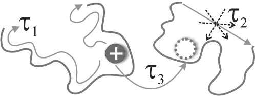
Figure 1: Time scales: $\tau_{1}$ is the time scale for intra-chain ionic motion (M1), $\tau_{2}$ is the relaxation time of the polymer chain (related to $\tau_{R}$: see text for details)(M2), and $\tau_{3}$ is the waiting time of an ion between two inter-chain jumps (M3).

Atomistic NVT MD simulations are performed for the system poly(ethylene) oxide (PEO) and LiBF₄ with a concentration of EO:Li=20:1 (EO: ether oxygen). The two body effective polarizable potential employed is described in Ref. Borodin et al. (2003). We have simulated this system for different chain lengths ($N=24$ and $N=48$) and at different temperatures (400 K $\leq T\leq$ 450 K). The respective densities have been chosen to set the average pressure to values of the order of 1 MPa. This letter discusses the results for the $N=48$ system at $T=450$ K unless specified otherwise.

As has been observed before Borodin et al. (2003); Borodin and Smith (1998); Neyertz and Brown (1996); Müller-Plathe and van Gunsteren (1995) a Li⁺ ion is, most of the time, coordinated to a single polymer chain through EO atoms, interrupted by infrequent transitions between different chains. A Li⁺ ion which is bound to a polymer chain is coordinated to a few ($\approx 5$) and mostly contiguous oxygen atoms. After serially indexing the oxygen atoms of a chain in succession we mark the position of the Li⁺ at the chain by the average index, $n(t)$, of the enumerated oxygen atoms that belong to its coordination sphere. To elucidate (M1), we determine the average-square variation $\langle\Delta n(t)^{2}\rangle$ of the average oxygen index under the constraint that the Li⁺ ion is attached to the same chain during the time interval of length $t$. The result is shown in Fig.2. To a good approximation one observes diffusive dynamics $\langle\Delta n(t)^{2}\rangle=2D_{1}t$ where $D_{1}$ is the intra-chain ionic diffusivity. To account for the slight deviations from linear behavior we choose $D_{1}=\langle\Delta n(\tau_{2})^{2}\rangle/2\tau_{2}$ ($\tau_{2}$ defined in the next paragraph). For later purposes we define

$$\tau_{1}=(N-1)^{2}/\pi^{2}D_{1}$$ (1)

where $\tau_{1}$ is a measure of the time it takes for the lithium ion to diffuse from one end to the other end of the polymer chain. Here we obtain $\tau_{1}\approx 150$ ns (with $D_{1}$ from Fig.2).

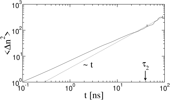
Figure 2: Average square variation of the average oxygen index of one chain to which a Li⁺ is associated during time interval $t$.

To characterize (M2) we first analyze the polymer dynamics. In Fig.3(a) we display the MSD $g_{O}(t)$ for an average oxygen atom (i.e. all oxygen atoms were considered for analysis irrespective of the presence or absence of Li⁺ near an oxygen atom), characterizing the dynamics of the polymer segments. According to our general procedure all MSD-functions are computed relative to the polymer c.o.m. It exhibits a Rouse-like behavior Rouse (1953); Doi and Edwards (2003) for short times $g_{O}(t)\propto t^{\alpha}$ with $\alpha\approx 0.6$, saturating at $g_{O}(t)\approx R_{e}^{2}/3$ where $R_{e}^{2}$ is the mean square end-to-end distance of the polymer . We have included the theoretical Rouse prediction, obtained via numerical summation

$$g(t/\tau_{R})=\frac{2R_{e}^{2}}{\pi^{2}}\sum_{p=1}^{N-1}\frac{1-\exp(-\frac{p^{2}t}{\tau_{R}})}{p^{2}}$$ (2)

where $\tau_{R}$ and $p$ denote Rouse time and mode number, respectively, and the sum is calculated over the $N-1$ eigenmodes. It yields a reasonable description of the observed MSD, using $\tau_{R}=19$ ns; see also Kreer et al. (2001). Qualitatively, it is expected that the oxygen atoms which are temporarily bound to a Li⁺ ion ought to be somewhat slower due to the decrease in the local degrees of freedom. This was checked by calculating $g_{O}^{bound}(t)$ for those oxygen atoms which, during the whole time interval of length $t$, are bound to one Li⁺ ion. Indeed, $g_{O}^{bound}(t)$ is also consistent with the Rouse prediction, using a longer Rouse time $\tau_{2}=42$ ns. Naturally, $\tau_{2}/\tau_{R}>1$ reflects the immobilization of the polymer segments due to the ions. Note that for longer $t$ less oxygen atoms contribute to this curve so that the statistics gets worse.

Switching to the Li⁺ dynamics, we first calculate the MSD $g_{Li}^{M2}$(t) of Li⁺ ions for which $|n(t)-n(0)|\leq 1$; see Fig.3(a). For $t>2$ ns this curve is close to $g_{O}^{bound}(t)$. Thus, we can conclude that the Li⁺ motion strictly follows the oxygen dynamics in the absence of (M1). In other words, the cations and the polymer segments exhibit coupled dynamics. Additionally, we find that for shorter times the Li⁺ ions are slower than the corresponding oxygen atoms.

In the absence of ion jump events between chains (M3) one would have $D_{M}=0$. We have identified the jumps from a microscopic analysis of the trajectories. On average after $\tau_{3}=110$ ns a Li⁺ ion jumps between two chains. To characterize the effect of these jumps we have first determined $g_{Li}^{M123}(t)$ which is the MSD of a Li⁺ ion between times $[t_{0}-t,t_{0}+t]$ if at time $t_{0}$ a jump happens and during the intervals $[t_{0}-t,t_{0}]$ and $[t_{0},t_{0}+t]$ the ion stays with the same chain, respectively. The MSD is averaged over all jumps (Fig.3(b)). Furthermore we have determined the MSD $g_{Li,\pm}^{M12}(t)$ during the intervals $[t_{0}-t,t_{0}]$ or $[t_{0},t_{0}+t]$, i.e. just before or after an inter-chain jump, respectively. For symmetry reasons one has $g^{M12}_{Li,+}(t)=g^{M12}_{Li,-}(t)\equiv g^{M12}_{Li}(t)$. If, additionally, the inter-chain jump at $t_{0}$ serves as a renewal process, the statistical independence of cationic dynamics before and after the jump requires $g_{Li}^{M123}(t)=g^{M12}_{Li,+}(t)+g^{M12}_{Li,-}(t)=2g^{M12}_{Li}(t)$. In case of correlations a smaller factor is expected compared to 2. As exhibited in Fig.3b this relation is indeed found with minor deviations (prefactor 2.2 instead of 2.0), thus validating the fact that inter-chain transitions can be regarded as renewal processes.

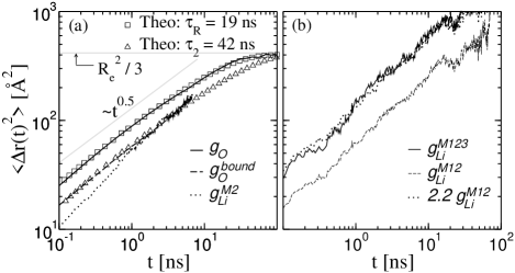
Figure 3: (a) MSD of (i) all oxygen atoms (solid), (ii) oxygen atoms which are bound to one $Li^{+}$ during time duration $t$ (dash), (iii) $Li^{+}$ which changed the average index of its oxygen neighbors by at most 1 (dot). Also shown are the Rouse predictions with $\tau_{R}$=19 ns ($\scriptstyle{\square}$) and $\tau_{2}$=42 ns ($\scriptstyle{\triangle}$). (b) MSD of Li⁺ under different constraints (see text).

In the following, we derive an explicit expression $D_{M}=D_{M}(\tau_{1},\tau_{2},\tau_{3})$. Based on the observed correlations between a Li⁺ ion and the polymer dynamics, $g_{Li}^{M12}(t)$ can be described by taking into account the Rouse dynamics (M2) plus the additional intra-chain diffusion (M1). Formally, one can write

$$g_{Li}^{M12}(t)=\langle(\vec{r}_{j}(t)-\vec{r}_{i}(0))^{2}\rangle_{M12}$$ (3)

The average is over the probability density that the initial oxygen index to which an ion is linked is $i$ and at a time $t$ later is $j$ and the distribution of monomer displacements as predicted in the Rouse theory. From Ref.Doi and Edwards (2003) one obtains, using $\langle\cos^{2}(p\pi(j-0.5)/N)\rangle_{M1}=1/2$ and $\langle\cos(p\pi(i+j-1)/N)\rangle_{M1}=0$,

$$g_{Li}^{M12}(t)=\frac{2R_{e}^{2}}{\pi^{2}}\sum_{p=1}^{N-1}\frac{1-\langle\cos\frac{p\pi(i-j)}{N}\rangle_{M1}\exp(-\frac{p^{2}t}{\tau_{2}})}{p^{2}}.$$ (4)

Assuming Gaussian dynamics for (M1), i.e. $\langle\Delta n^{2}\rangle\propto t$ (correction to the deviation as observed in Fig.2 can be easily implemented but are not of relevance here), one finds $\langle\cos(p\pi(i-j)/N)\rangle_{M1}=\exp(-p^{2}t/\tau_{1})$. Eq. 4 simplifies to (using Eq.2)

$$g_{Li}^{M12}(t)=g(t/\tau_{12})$$ (5)

with $1/\tau_{12}=1/\tau_{1}+1/\tau_{2}$. Thus, the dynamical effects of (M1) and (M2) appear through the resulting relaxation rate $1/\tau_{12}$. Finally, using the renewal property one can write $D_{M}=a_{M}^{2}/6\tau_{3}$ explicitly as

$$D_{M}=\langle g_{Li}^{M12}(\tau)\rangle_{M3}/6\tau_{3}$$ (6)

where a${}_{M}^{2}$ corresponds to the average MSD between successive inter-chain hopping events due to (M1) and (M2). The average is taken over the distribution of time intervals between these events. For the numerical analysis (see below) we take a simple exponential distribution.

Approximate analytical expressions can be obtained by converting the sum in Eq.4 into an integral from 0 to $\infty$ Doi and Edwards (2003). Then one obtains $g_{Li}^{M12}=2R_{e}^{2}\pi^{-3/2}\sqrt{t/\tau_{12}}$ for $t\ll\tau_{12}$ and $g_{Li}^{M12}=R_{e}^{2}/3$ for $t\gg\tau_{12}$, respectively. Inserting these results into Eq.6 gives

$$D_{M} =\frac{R_{e}^{2}}{6\pi}\sqrt{\frac{1}{\tau_{3}\tau_{12}}} \tau_{3}\ll\tau_{12}$$ if (7a)

$$=\frac{R_{e}^{2}}{18\tau_{3}} \tau_{3}\gg\tau_{12}$$ if (7b)

The scaling of $D_{M}$ with $\tau_{3}$ in Eq.(7a) is consistent with the numerical results, obtained in Ref.Borodin and Smith (2006). Eq.(7a) holds for long chains and takes into consideration the implicit correlations of (M1) and (M2). By neglecting these correlations, as done in Ref.Borodin and Smith (2006), the term $\sqrt{1/\tau_{12}}=\sqrt{1/\tau_{1}+1/\tau_{2}}$ would instead become $\sqrt{1/\tau_{1}}+\sqrt{1/\tau_{2}}$. This would largely overestimate $D_{M}$ (for instance, in PEO/LiBF₄ by 35 %) and the contribution of (M1) for the case $\tau_{3}\ll\tau_{12}$.

In contrast to the DBP-model we obtain $D_{M}\propto 1/\tau_{ren}$ only for short chains. The main conclusion, however, that the Li⁺ diffusion has the same temperature dependence as the inverse Rouse time and thus as the polymer dynamics, remains valid because all the three time scales $\tau_{i}$ have a similar temperature dependence (data not shown).

In Tab.I we have compiled $\tau_{1}$, $\tau_{2}$, $\tau_{3}$, obtained from our simulations for $N=24$ and $N=48$. Of major importance are their scaling properties with $N$. One expects $\tau_{1},\tau_{2}\propto N^{2}$ and $\tau_{3}\propto N^{0}$. Considering the appropriate number of eigenmodes, the predictions for $N=24$, based on $N=48$, are given in parenthesis. The agreement is convincing.

$N$	$\tau_{1}$ [ns]	$\tau_{2}$ [ns]	$\tau_{3}$ [ns]
48	150	42	110
24	34 (36)	10 (10)	90 (110)

Table 1: The relevant time scales $\tau_{i}$ for $N=48$ and $N=24$ as well as a check of the scaling relations.

By setting $\tau_{1}\rightarrow\infty$ one can estimate the contribution of (M1) to $D_{M}$ in the limit of long chains ($\tau_{3}\ll\tau_{12}$). It is as small as 12% for the present system.

Naively one might expect that $a_{M}^{2}\propto N^{0}$ and thus $D_{M}\propto N^{0}$ for all $N$, see e.g. Shi and Vincent (1993), because (M1)-(M3) are related to local motions. Using the scaling results for the $\tau_{i}$ one obtains, however, $D_{M}\propto N^{0}$ only for long chains $(\tau_{3}\ll\tau_{12})$ whereas $D_{M}\propto N$ for short chains. The reason is that for short chains $a_{M}^{2}$ is limited by the end-to-end distance of the polymer which brings an $N$-dependence.

In the present case, the crossover in $D_{M}$, i.e. $\tau_{3}\approx\tau_{12}$, occurs for $N\approx 100$ (see inset of Fig.4). It has been speculated Shi and Vincent (1993) that the emergence of the entanglement regime ($N\approx 75$ Shi and Vincent (1993); Appel and Fleischer (1993)) leads to the crossover with an accompanying change of cation conduction process from polymer c.o.m dominated motion to percolation type transport (i.e. (M3)). However, we find, it is a coincidence that the entanglement length is similar to the crossover length. Thus, the crossover to $D_{M}\propto N^{0}$ is physically unrelated to entanglement effects.

We can predict the $N$-dependence of $D_{Li}(N)$ for a large range of $N$ values by combining the empirical $N$-scaling von Meerwall et al. (1998); Hayamizu et al. (2002) (see inset Fig.4) of $D_{c.o.m}(N)$ with $D_{M}(N)$. The Rouse scaling ($D_{c.o.m}\propto N^{-1}$) is known to be violated and substantially higher exponents ($\geq 1.5$) have been reported Paul and Smith (2004); von Meerwall et al. (1998); Hayamizu et al. (2002).

To determine $D_{M}(N)$ we have used Eq.5 and 6 by explicitly calculating the sum in Eq.4. Fig.4 displays the predicted $D_{Li}(N)$ along with the experimental data from Ref.Shi and Vincent (1993). In agreement, both indicate a transition to a $N$-independent regime beyond $N\approx 100$. Further included in Fig.4 is an estimation of $D_{Li}$ under the assumption that no entanglement effects are present for $D_{c.o.m}$ by simply extending the scaling in the Rouse-regime to all $N$. As expected, the large-N behavior does not depend on the specific form of $D_{c.o.m}$. However, one might speculate that the appearance of the minimum in $D_{M}(N)$ is indicative of entanglement effects.

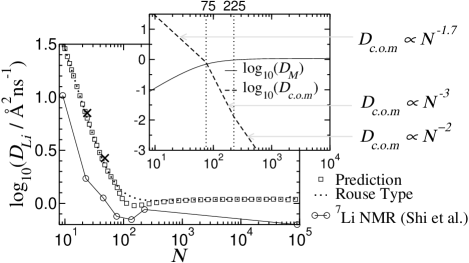
Figure 4: Self diffusivity of Li⁺, $D_{Li}=D_{M}+D_{c.o.m}$ with D_M from Eq.6 ($\scriptstyle{\square}$). The dotted line shows the prediction for a pure Rouse-type motion. ExperimentalShi and Vincent (1993) $D_{Li}$ for PEO:LiCF₃SO₃ with EO:Li=20:1 at T=342 K is included ($\circ$). The inset shows $D_{M}$ and $D_{c.o.m}$ individually. $D_{Li}$ values obtained from simulations are marked by crosses.

Interestingly, within the present approach the value of $\tau_{3}$ can be estimated from experimental data. For very large $N=N_{L}$ one has (see Eq.(7a)) $\tau_{3}=(N_{s}b^{2}/(6\pi D_{Li}|_{N=N_{L}}))^{2}/(\tau_{2}|_{N=N_{S}})$ where $b$ is the statistical segment length of the polymer, $\tau_{2}/\tau_{R}\approx 2.2$ and $\tau_{R}|_{N=N_{S}}$ can be estimated from $D_{c.o.m}\approx D_{Li}|_{N=N_{S}}$ (at some small $N=N_{S}$) using the Rouse prediction. For the experimental data in Fig.4 this yields $\tau_{3}\approx 80$ ns. Via NMR experiments Hayamizu et al. (2002) local relaxation processes may be probed to extract information about $\tau_{1}$.

It is likely that the identified motional mechanisms are generally applicable to understand the ionic dynamics in different polymer electrolytes. Furthermore we checked that the presence of a small fraction of ions which are, temporarily, not bound to a polymer does not change the value of $D_{M}$ by more than 10%. Of course, corrections will become relevant for larger ion concentration due to their mutual interaction. Note that our approach averages over the different structural realizations and thus include, e.g., temporary complexation of an ion by two polymer chains.

In summary, we have elucidated ion dynamics in polymer electrolytes by extracting microscopic properties from simulation and expressing them in analytical terms. This extends previous phenomenological approaches like the dynamic bond-percolation model, by assigning its key concept, i.e. the presence of renewal processes, a specific microscopic interpretation. For long chains the scaling relation $D_{Li}\propto 1/\sqrt{\tau_{12}\cdot\tau_{3}}$ is obtained which goes beyond the expressions from the DBP model. In any event, for the transport of lithium ions fast transitions of ions between different chains are vital. Since the expression $D_{Li}(\tau_{1},\tau_{2},\tau_{3})$ is now available one can estimate the possible range of ionic mobilities for linear chain polymer electrolytes for all $N$.

We would like to thank M. Vogel for important discussions and a critical reading of the manuscript and Y. Aihara, J. Baschnagel, O. Borodin, K. Hayamizu, and M. Ratner for helpful correspondence.

References

- Gray (1991) F. M. Gray, Solid Polymer Electrolytes (Wiley-VCH, New York, 1991).
- Bruce and Vincent (1993) P. G. Bruce and C. A. Vincent, J. Chem. Soc. Faraday Trans. 89, 3187 (1993).
- Ratner and Shriver (1988) M. A. Ratner and D. F. Shriver, Chem. Rev. 88, 109 (1988).
- Ratner et al. (2000) M. Ratner, P. Johansson, and D. Shriver, MRS Bulletin 25, 31 (2000).
- Borodin et al. (2003) O. Borodin, G. D. Smith, and R. Douglas, J. Phys. Chem. B 107, 6824 (2003).
- Lammert et al. (2003) H. Lammert, M. Kunow, and A. Heuer, Phys. Rev. Lett. 90, 215901 (2003).
- Nitzan and Ratner (1994) A. Nitzan and M. A. Ratner, J. Phys. Chem. 98, 1765 (1994).
- Allen and Tildesley (2004) M. P. Allen and D. J. Tildesley, Computer Simulation of Liquids (Clarendon, Oxford, 2004).
- Müller-Plathe and van Gunsteren (1995) F. Müller-Plathe and W. van Gunsteren, J. Chem. Phys. 103, 4745 (1995).
- Neyertz and Brown (1996) S. Neyertz and D. Brown, J. Chem. Phys. 104, 3797 (1996).
- Borodin and Smith (1998) O. Borodin and G. D. Smith, Macromolecules 31, 8396 (1998).
- Siqueira and Ribeiro (2006) L. J. A. Siqueira and M. Ribeiro, J. Chem. Phys. 125, 214903 (2006).
- Borodin and Smith (2006) O. Borodin and G. D. Smith, Macromolecules 39, 1620 (2006).
- Borodin et al. (2006) O. Borodin, G. D. Smith, O. Geiculescu, S. Creager, B. Hallac, and D. DesMarteau, J. Phys. Chem. B 110, 24266 (2006).
- Doi and Edwards (2003) M. Doi and S. Edwards, The Theory of Polymer Dynamics (Oxford Science Publications, 2003).
- Rouse (1953) P. E. Rouse, J. Chem. Phys. 21, 1272 (1953).
- Kreer et al. (2001) T. Kreer, J. Baschnagel, M. Müller, and K.Binder, Macromolecules 34, 1105 (2001).
- Shi and Vincent (1993) J. Shi and C. A. Vincent, Solid State Ionics 60, 11 (1993).
- Appel and Fleischer (1993) M. Appel and G. Fleischer, Macromolecules 26, 5520 (1993).
- von Meerwall et al. (1998) E. von Meerwall, S. Beckman, J. Jang, and L. Mattice, J. Chem. Phys. 108, 4299 (1998).
- Hayamizu et al. (2002) K. Hayamizu, E. Akiba, T. Bando, and Y. Aihara, J. Chem. Phys. 117, 5929 (2002).
- Paul and Smith (2004) W. Paul and G. D. Smith, Rep. Prog. Phys. 67, 1117 (2004).