Electron turbulence at nanoscale junctions

Abstract

Electron transport through a nanostructure can be characterized in part using concepts from classical fluid dynamics. It is thus natural to ask how far the analogy can be taken, and whether the electron liquid can exhibit nonlinear dynamical effects such as turbulence. Here we present an ab-initio study of the electron dynamics in nanojunctions which reveals that the latter indeed exhibits behavior quite similar to that of a classical fluid. In particular, we find that a transition from laminar to turbulent flow occurs with increasing current, corresponding to increasing Reynolds numbers. These results reveal unexpected features of electron dynamics and shed new light on our understanding of transport properties of nanoscale systems.

Electron transport through a nanoscale junction is usually described as a scattering problem.Landauer (1957); Büttiker et al. (1985); Di Ventra et al. (2000); Taylor et al. (2001); Damle et al. (2001); Palacios et al. (2002) On the other hand, it has been shownMartin and Schwinger (1959); Vignale et al. (1997); Tokatly (2005); D’Agosta and Di Ventra (2006) that the behavior of the electron liquid obeys dynamical equations of motion which are similar in form to those governing the dynamics of classical liquids. In particular, it was recently shownD’Agosta and Di Ventra (2006) that the time-dependent Schrödinger equation (TDSE) for electrons flowing across a nanostructure can be cast in the form of generalized Navier-Stokes equations. A consequence of this analogy is the prediction that under certain conditions the laminar flow of the liquid may become unstable and turbulent behavior is expected.D’Agosta and Di Ventra (2006); Frisch (1995); Landau and Lifshitz (1987) One can then borrow knowledge from classical fluid dynamics and hypothesize that the electron flow will make a transition from laminar to turbulent regimes, if, e.g., the current is increased. Like in a classical liquid, if, for instance, electrons flow from one electrode (call it the top electrode) to another (call it the bottom electrode) across a nanojunction, turbulence would first manifest itself with the break-up of the top-down symmetry of the electron flow.Frisch (1995); Landau and Lifshitz (1987) By increasing the current further one should observe the formation of eddies in proximity to the junction. These eddies are created because of the larger kinetic energy in the direction of current flow (longitudinal kinetic energy) compared to the transverse direction (transverse kinetic energy). By increasing the current further, the disparity between longitudinal and transverse components of the kinetic energy increases, and the system flow eventually breaks any remaining symmetry, thus fully developing turbulence.Frisch (1995); Landau and Lifshitz (1987) Despite the prediction of turbulent behavior of the electron liquid in nanostructuresD’Agosta and Di Ventra (2006) an explicit demonstration of this phenomenon and the analysis of its microscopic features has not been presented yet.

In this communication we set to show numerically turbulent effects for the electron liquid crossing a nanojunction both by solving directly the TDSE, and by solving the generalized Navier-Stokes equations derived in Ref. D’Agosta and Di Ventra, 2006. These read

$$D_{t}n({\bf r},t)= -n({\bf r},t){\bf\nabla}\cdot{\bf u}({\bf r},t)\,,$$

$$mn({\bf r},t)D_{t}u_{i}({\bf r},t)= -\partial_{i}P({\bf r},t)+\partial_{j}\pi_{i,j}$$ (1)

$$-n({\bf r},t)\partial_{i}V_{\rm ext}({\bf r},t)\,.$$

Here, $n$ is the electron density, ${\bf u}={\bf j}/n$ is the velocity field, i.e. the ratio between the current density ${\bf j}$ and the density, and $D_{t}=\frac{\partial}{\partial t}+{\bf u}\cdot\nabla$ is the convective derivative.Landau and Lifshitz (1987) $P({\bf r},t)$ is the pressure of the liquid, $V_{\rm ext}({\bf r},t)$ an external potential, and $\pi_{i,j}$ is a traceless tensor that describes the shear effect on the liquid. It has the form

$$\pi_{i,j}=\eta\left(\partial_{i}u_{j}+\partial_{j}u_{i}-\frac{2}{3}\delta_{i,j}\partial_{k}u_{k}\right)\,,$$ (2)

where $\eta=\hbar nf(n)$ is the viscosity of the electron liquid and $f(n)$ is a smooth function of the density.Conti and Vignale (1999)

In analogy with the classical case we expect that the atomic structure, and in particular atomic defects in proximity to the junction, play the role of “obstacles” for the liquid and thus favor turbulence. Since we aim at showing that turbulence develops irrespective of the underlying atomic structure, we consider electrons interacting with a uniform positive background charge (i.e., the “jellium” modelDi Ventra and Lang (2002)). The system we consider therefore consists of two large but finite jellium electrodes– subject to a bias– connected via a nanoscale jellium bridge. (The jellium edge of this system is represented with solid lines in each panel of Fig. 1.) We choose the density of the jellium at equilibrium typical of bulk gold ($r_{s}\approx 3a_{0}$). For computational convenience we choose a quasi-2D system, approximately 2.8 Å thick. Note that, everything else being equal, a quasi-2D geometry disfavors turbulence compared to a 3D one. We thus expect that if turbulence develops in our chosen quasi-2D geometry with given thickness, then turbulence will develop even more easily if we leave everything else unchanged (including the total current) and increase the thickness of the electrodes.

The solution of the TDSE for the many-body system is obtained within Time-Dependent Current Density Functional Theory(TDCDFT);Vignale et al. (1997) i.e., for each single-particle state $\phi_{\alpha}$, we have solved the equation of motion (in atomic units)

$$\left\{i\frac{\partial}{\partial t}-\frac{1}{2}\left(\frac{1}{i}{\bf\nabla}-\frac{1}{c}{\bf a}_{\rm xc}\right)^{2}-v_{\rm jel}-v_{\rm H}-v_{\rm xc}\right\}\phi_{\alpha}=0$$ (3)

where $c$ is the speed of light, $v_{\rm jel}$ is the potential due to the jellium, $v_{\rm H}$ is the Hartree potential, and $v_{\rm xc}$ is the exchange-correlation scalar potential. The shear viscosity of the electron liquid $\eta$ enters the problem through the exchange-correlation vector potential ${\bf a}_{\rm xc}$.Vignale et al. (1997); Conti and Vignale (1999) If we make the appoximation that, at any given time, the viscosity is a function of the density only, and does not depend on time explicitly, we find that the $i^{\rm th}$ component of ${\bf a}_{\rm xc}$ evolves according toConti and Vignale (1999)

$$\frac{1}{c}\frac{\partial a_{{\rm xc},i}}{\partial t}=\frac{1}{n}\sum_{j}\bigg{\{}\eta\frac{\partial^{2}u_{i}}{\partial r_{j}^{2}}+\frac{\eta}{3}\frac{\partial^{2}v_{j}}{\partial_{i}\partial_{j}}$$ (4)

$$+\frac{\partial\eta}{\partial r_{j}}\bigg{(}\frac{\partial u_{i}}{\partial r_{j}}+\frac{\partial u_{j}}{\partial r_{i}}\bigg{)}-\frac{2}{3}\frac{\partial\eta}{\partial r_{i}}\frac{\partial u_{j}}{\partial r_{j}}\bigg{\}}\,.$$

For the viscosity $\eta$ of the electron liquid we have used the one reported in Ref. Conti and Vignale, 1999. We employ the approach described in Refs. Di Ventra and Todorov, 2004; Bushong et al., 2005; Sai et al., ; Cheng et al., 2006 to initiate electron dynamics and calculate the current. We prepare the system by placing it in its ground state; because of the applied bias, the system exhibits a separation of charge. At a time $t=0$, we remove the bias, and let the system evolve according to eq. (3). After long time scales, the electrons encounter the far boundaries of the jellium electrodes and reflect. However, we are interested in comparing the electron dynamics calculated from eq. (3) with the one obtained by solving the Navier-Stokes equations (1), at times smaller than this reflection time. Equations (1) are solved by assuming the same density, initial velocity and viscosity of the liquid employed in the TDCDFT calculation. We also solve eqs. (1) assuming the liquid to be incompressible. This simplifies the calculations enormously but leads to some minor differences with the solutions of eq. (3) (see discussion later).

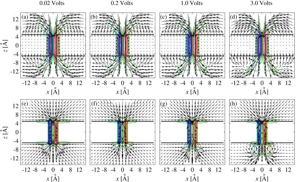
Figure 1: (Color online) Panels (a)-(d): Electron current density for electrons moving from the top electrode to the bottom electrode across a nanojunction at $t=1.4$ fs, for an initial bias of (a) 0.02 V, (b) 0.2 V, (c) 1.0 V and (d) 3.0 V. The arrows denote the current density, while the level sets denote the curl of the 2D current density. The solid lines delimit the contour of the junction. Panels (e)-(h): Velocity field solution of the equations (1), for a liquid with same velocity, density and viscosity as the quantum mechanical one.

Fig. 1 depicts the flow of electrons across the nanostructure, for a range of biases between 0.02V and 3.0V, after the initial transient. The panels (a)-(d) correspond to the solution of eq. (3); the panels (e)-(h) to the solution of the eqs. (1) using the same set of parameters.Popinet (2003) Panel (a) has to be compared with panel (e); panel (b) with (f), and so on. As anticipated, we observe some differences between the solutions of the eqs. (1) and the solutions of the eq. (3). These differences are due to the details of the charge configuration at the electrode-junction interface, and some degree of compressibility of the quantum liquid in the junction.

From Fig. 1 we can see the effect of surface charges, in that some electrons flow parallel to the surfaces.Sai et al. More importantly, at low biases, the flow is laminar and “smooth”. In addition, at these biases the current density shows an almost perfect top-bottom symmetry: the direction of the flow is symmetric with respect to the operation $z\rightarrow-z$. This symmetry is even more evident by comparing the curl of the current density in the top and bottom electrodes (see for instance Fig. 1(a) and (e)).

By increasing the bias, however, a transition occurs: the symmetry $z\rightarrow-z$ of the current density breaks completely, and eddies start to appear in proximity to the junction. This is clearly evident, for instance, in Fig. 1(d) and (h). The outgoing current density in the bottom electrode has a more varied angular behavior, in contrast to the behavior in the top electrode, in which the electron liquid flows more uniformly toward the junction.

Since the panels (e)-(h) of Fig. 1 practically describe the dynamics of a classical fluid with the same parameters as the quantum liquid, the analogy between the electron flow and the one of a classical liquid is quite evident. We can push this analogy even further by defining a Reynolds number for the quantum system as well: $R=u_{z}L\rho/\eta$, where $u_{z}$ is the longitudinal velocity in the junction, $L$ is the width of the junction, and $\rho$ is the density. Using the density of valence electrons in gold, and using the current density in the junction at $t=1.4$ fs, we obtain for the quantum case the following Reynolds numbers: 0.216, 2.16, 10.8 and 32.5 for 0.02 V, 0.2 V, 1.0 V, and 3.0 V, respectively.

Just like in the classical case, we can then reinterpret the above results as follows. At low Reynolds numbers, the flow is highly symmetric from top to bottom. This symmetry is lost as the Reynolds number is increased. At high Reynolds numbers, the incident flow is laminar, while the outgoing flow has a jet-like character, and “turns back” on itself creating local eddies in the current density.

Having shown the similarity between the current flow obtained using the Navier-Stokes equations (1) and the one obtained solving eq. (3) we can study the first one at times scales prohibitive for full quantum mechanical simulations. We can also study the effect of a larger thickness of the electrodes on the turbulent flow by realizing that this is equivalent to increasing the Reynolds number (which, incidentally, is also equivalent to increasing the bias). This is illustrated in Fig. 2 where the current density and the curl of the current density are plotted for the Reynolds number 32.5 of Fig. 1(h) (left panel of Fig. 2); same system but with a Reynolds number five times larger (middle panel of Fig. 2); and (right panel of Fig. 2) with a Reynolds number ten times larger.

From Fig. 2 it is evident that by increasing thickness the last remaining symmetry $x\rightarrow-x$ is broken at earlier times, leading to turbulent behavior closer to the junction. For instance, in the case represented in Fig. 2 (middle panel), the left-right symmetry is lost at about 14 fs, with consequent asymmetric flow within about 50 Å  from the junction center. For the structure represented in Fig. 2 (right panel), the symmetry is broken at about 6 fs, and the flow asymmetry appears at about 25 Å  from the junction.

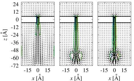
Figure 2: (Color online) Current density (arrows) and curl of the current density (denoted by level sets) of the electron liquid, for three different Reynolds numbers, 32.5 (left panel), 162 (middle panel), and 325 (right panel). Note that the fluid velocity has lost perfect left-right symmetry in the middle- and right-panel cases.

We can better quantify the amount of turbulence by calculating the velocity correlation tensorLandau and Lifshitz (1987)

$$B_{ik}=\langle(v_{i}({\bf r})-v_{i}({\bf r}+\delta{\bf r}))(v_{k}({\bf r})-v_{k}({\bf r}+\delta{\bf r}))\rangle\,,$$ (5)

where $\delta{\bf r}$ is a given distance, and $i,k=x,y,z$. Here, the angle brackets $\langle\cdots\rangle$ denote averaging over all positions ${\bf r}$ within a given region. Fully developed and isotropic turbulence has a velocity correlation tensor that is a function only of the magnitude of $\delta{\bf r}$, and increases quadratically with distance.Landau and Lifshitz (1987) Instead, the turbulence in the examples of Fig. 2 is not fully developed. The velocity correlation tensor, $B_{ik}$, thus depends on both the magnitude of $\delta{\bf r}$ as well as its direction. This is illustrated in Fig. 3 where various components of $B_{ik}$ are plotted at $t=75.0$ fs for the system with Reynolds number 32.5 as a function of the magnitude of $\delta{\bf r}$, where we have chosen $\delta{\bf r}$ to point in the longitudinal (z) direction. The spatial averaging has been carried out over the left-hand side of the outgoing region (that is, in the region $z$ = [-27.3 Å, -72.1 Å], $x$ = [-25.9 Å, 0.0 Å], where the origin is in the center of the junction). For comparison, the same quantity is plotted for the laminar case, i.e. for a Reynolds number of .216. (To compare the laminar and turbulent cases we have scaled the average turbulent velocity to the average laminar velocity.) As expected, in the laminar case the correlation tensor is essentially zero, while for the turbulent case it increases with distance.

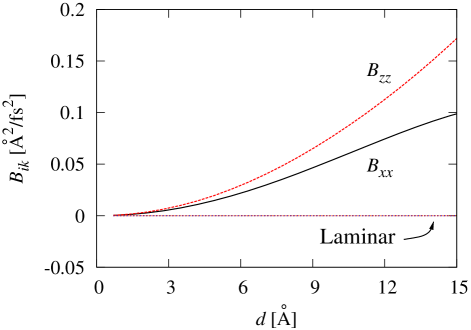
Figure 3: (Color online) Various components of the velocity correlation tensor $B_{ik}$ as a function of distance $d=|\delta{\bf r}|$, for a Reynolds number of $R=32.5$. For the case where $R=0.216$, the elements of $B_{ik}$ are orders of magnitude smaller, and so the corresponding curves for the laminar case coincide with the x axis.

We conclude by noting that an experiment in which the electron flow can be monitored directly may measure nonlaminar electron behavior as an asymmetry between the incoming and outgoing patterns of the current density through a nanojunction. Experiments similar to the ones reported in Ref. Topinka et al., 2000, which use scanning probe microscopy to image the flowlines, may provide such capabilities. Note, however, that since these scanning probe techniques record images over time scales much longer than the turbulent electron dynamics, one would expect that in the turbulent regime images of current flow appear “smeared out” compared to the laminar case, and asymmetric in the incoming and outgoing patterns. From the present work and the analytical results obtained in Ref. D’Agosta and Di Ventra, 2006, we also suggest that fully 3D and non-adiabatic junctions, i.e. junctions with a geometry that changes abruptly (like the one explored in this work), are the best candidates to observe turbulence. We also expect defects and other impurities to favor turbulent behavior by playing the role of “obstacles” for the electron flow.

We finally note that turbulent behavior may have consequences on the formation (or lack thereof) of local equilibrium distributions in the electrodes,Bushong et al. (2005) and may generate non-trivial local electron heating effects in the junctionD’Agosta et al. (2006) and at the eddies sites; phenomena and properties which are still poorly understood at the nanoscale and ultimately may have unexpected consequences on the stability of nanostructures under current flow.Huang et al. (2006)

We acknowledge useful discussions with Roberto D’Agosta. One of us (JG) received support from the National Science Foundation’s REU program. This work was supported by the U.S. Department of Energy under grant DE-FG02-05ER46204.

References

- Landauer (1957) R. Landauer, IBM J. Res. Dev. 1, 223 (1957).
- Büttiker et al. (1985) M. Büttiker, Y. Imry, R. Landauer, and S. Pinhas, Phys. Rev. B 31, 6207 (1985).
- Di Ventra et al. (2000) M. Di Ventra, S. T. Pantelides, and N. D. Lang, Phys. Rev. Lett. 84, 979 (2000).
- Taylor et al. (2001) J. Taylor, H. Guo, and J. Wang, Phys. Rev. B 63, 245407 (2001).
- Damle et al. (2001) P. S. Damle, A. W. Ghosh, and S. Datta, Phys. Rev. B 64, 201403(R) (2001).
- Palacios et al. (2002) J. J. Palacios, A. J. Pérez-Jiménez, E. Louis, E. SanFabián, and J. A. Vergés, Phys. Rev. B 66, 035322 (2002).
- Martin and Schwinger (1959) P. C. Martin and J. Schwinger, Phys. Rev. 115, 1342 (1959).
- Vignale et al. (1997) G. Vignale, C. A. Ullrich, and S. Conti, Phys. Rev. Lett. 79, 4878 (1997).
- Tokatly (2005) I. V. Tokatly, Phys. Rev. B 71, 165104 (2005).
- D’Agosta and Di Ventra (2006) R. D’Agosta and M. Di Ventra, J. Phys.: Condens. Matter 18, 11059 (2006).
- Frisch (1995) U. Frisch, Turbulence (Cambridge University Press, 1995).
- Landau and Lifshitz (1987) L. D. Landau and E. M. Lifshitz, Fluid Mechanics, vol. 6 of Course of Theoretical Physics (Pergamon Press, NY, 1987), 2nd ed.
- Conti and Vignale (1999) S. Conti and G. Vignale, Phys. Rev. B 60, 7966 (1999).
- Di Ventra and Lang (2002) M. Di Ventra and N. D. Lang, Phys. Rev. B 65, 045402 (2002).
- Di Ventra and Todorov (2004) M. Di Ventra and T. N. Todorov, J. Phys. Cond. Matt. 16, 8025 (2004).
- Bushong et al. (2005) N. Bushong, N. Sai, and M. Di Ventra, Nano Lett. 5, 2569 (2005).
- (17) N. Sai, N. Bushong, R. Hatcher, and M. Di Ventra, Phys. Rev. B, in press.
- Cheng et al. (2006) C.-L. Cheng, J. S. Evans, and T. V. Voorhis, Phys. Rev. B 74, 155112 (2006).
- Popinet (2003) S. Popinet, J. Comput. Phys. 190, 572 (2003).
- Topinka et al. (2000) M. A. Topinka, B. J. LeRoy, S. E. J. Shaw, E. J. Heller, R. M. Westervelt, K. D. Maranowski, and A. C. Gossard, Science 289, 2323 (2000).
- D’Agosta et al. (2006) R. D’Agosta, N. Sai, and M. Di Ventra, Nano Lett. 6, 2935 (2006).
- Huang et al. (2006) Z. F. Huang, B. Q. Xu, Y.-C. Chen, M. Di Ventra, and N. J. Tao, Nano Lett. 6, 1240 (2006).
- Kohn and Sham (1965) W. Kohn and L. Sham, Phys. Rev. 140, A1133 (1965).
- Zangwill and Soven (1980) A. Zangwill and P. Soven, Phys. Rev. Lett. 45, 204 (1980).
- Runge and Gross (1984) E. Runge and E. K. U. Gross, Phys. Rev. Lett. 52, 997 (1984).
- Ceperley and Alder (1980) D. M. Ceperley and B. J. Alder, Phys. Rev. Lett. 45, 566 (1980).
- Perdew and Zunger (1981) J. P. Perdew and A. Zunger, Phys. Rev. B 23, 5048 (1981).
- Tal-Ezer and Kosloff (1984) H. Tal-Ezer and R. Kosloff, J. Chem. Phys. 81, 3967 (1984).