Quantum Impurity Entanglement

Abstract

Entanglement in $J_{1}-J_{2}$, $S=1/2$ quantum spin chains with an impurity is studied using analytic methods as well as large scale numerical density matrix renormalization group methods. The entanglement is investigated in terms of the von Neumann entropy, $S=-\Tr\rho_{A}\log\rho_{A}$, for a sub-system $A$ of size $r$ of the chain. The impurity contribution to the uniform part of the entanglement entropy, $S_{imp}$, is defined and analyzed in detail in both the gapless, $J_{2}\leq J_{2}^{c}$, as well as the dimerized phase, $J_{2}>J_{2}^{c}$, of the model. This quantum impurity model is in the universality class of the single channel Kondo model and it is shown that in a quite universal way the presence of the impurity in the gapless phase, $J_{2}\leq J_{2}^{c}$, gives rise to a large length scale, $\xi_{K}$, associated with the screening of the impurity, the size of the Kondo screening cloud. The universality of Kondo physics then implies scaling of the form $S_{imp}(r/\xi_{K},r/R)$ for a system of size $R$. Numerical results are presented clearly demonstrating this scaling. At the critical point, $J_{2}^{c}$, an analytic approach based on a Fermi liquid picture, valid at distances $r\gg\xi_{K}$ and energy scales $T\ll T_{K}$, is developed and analytic results at $T=0$ are obtained showing $S_{imp}=\pi\xi_{K}[1+\pi(1-{r}/{{R}})\cot({\pi r}/{{R}})]/(12R)$ for finite $R$. For $T>0$, in the thermodynamic limit, we find $S_{imp}=[\pi^{2}\xi_{K}T/(6v)]\coth(2\pi rT/v)$. In the dimerized phase an appealing picture of the entanglement is developed in terms of a thin soliton (TS) ansatz and the notions of impurity valence bonds (IVB) and single particle entanglement (SPE) are introduced. The TS-ansatz permits a variational calculation of the complete entanglement in the dimerized phase that appears to be exact in the thermodynamic limit at the Majumdar-Ghosh point, $J_{2}=J_{1}/2$, and surprisingly precise even close to the critical point $J_{2}^{c}$. In appendices the TS-ansatz is further used to calculate $\langle S^{z}_{r}\rangle$ and $\langle\vec{S}_{r}\cdot\vec{S}_{r+1}\rangle$ with high precision at the Majumdar-Ghosh point and the relation between the finite temperature entanglement entropy, $S(T)$, and the thermal entropy, $S_{th}(T)$, is discussed. Finally, the alternating part of $S_{imp}$ is discussed, together with its relation to the boundary induced dimerization.

1 Introduction

Much of the mystery and power of quantum mechanics arises from entanglement, which leads to Einstein’s “spooky action at a distance” but is now recognized as a resource by the quantum information community, being essential for quantum teleportation or quantum computing [1]. Ground states of quantum field theories and many body theories exhibit fascinating entanglement properties which are beginning to be understood [2, 3, 4, 5, 6, 7]. A useful measure of many body entanglement when the total system is in a pure state is the von Neumann entanglement entropy. This is obtained by focusing on bipartite system where space can be divided into 2 regions, $A$ and $B$. Beginning with the ground state pure density matrix, region $B$ is traced over to define the reduced density matrix $\rho_{A}$. From this the von Neumann entanglement entropy [8, 9],

$$S(r)\equiv-\Tr[\rho_{A}\ln\rho_{A}]$$ (1.1)

is obtained for subsystem of size $r$. Several other measures of entanglement are in current use such as the concurrence [10, 11] which is monotonically related to the entanglement of formation [12], the distillable entanglement [12, 13] and the relative entropy of entanglement [14, 15, 16]. See also [17]. Some of these measures have been developed to describe entanglement as it occurs in systems in a mixed state where it is much harder to quantify entanglement, see for instance the seminal paper by Bennett et al. [12]. Here we focus mainly on bipartite systems in pure states for which the von Neumann entropy, $S$, is an essentially unique measure of the entanglement. The rate at which $S$ grows with the spatial extent, $r$, of region $A$ is not only a fundamental measure of entanglement, it is also crucial [18, 19, 20, 21] to the functioning of the Density Matrix Renormalization Group (DMRG) a powerful numerical method for solving many body problems [22, 23]. For systems with finite correlation lengths, it is generally expected that $S_{A}$ grows with the area of the boundary of region $A$ [24, 25]. In the one-dimensional case, conformally invariant systems (with infinite correlation length) have $S(r)\to(c/3)\ln r$ [2, 26] where $c$ is the “central charge” characterizing the conformal field theory (CFT). Entanglement entropy has recently been shown to be a useful way of characterizing topological phases of many body theories [27, 28, 29, 30], which cannot be characterized by any standard order parameter. Entanglement entropy is also closely related to the thermodynamic entropy of black holes and to the “holographic principle” relating bulk to boundary field and string theories [29, 31, 32]. Hence, due to these latter developments, even though the von Neumann entanglement entropy may only give an incomplete description of entanglement in mixed states, such as would be the case at finite temperature or in the presence of noise from the environment, an understanding of its behavior in such states is important from the condensed matter perspective. We discuss the precise connection between the finite temperature entanglement entropy and the thermal entropy in some detail in E.

Recent experiments [33] on the magnetic salt LiHo_xY_1-xF₄ have been interpreted as evidence for quantum entanglement in the magnetic susceptibility and electronic specific heat at temperatures approaching 1K. Theoretical work have shown that macroscopic entanglement is in principle observable at much higher temperatures [34] and should also be observable using other probes such as neutron scattering [35]. Experimental measures of the concurrence have thus been obtained [33, 35]. Some of the theoretical [36, 37, 38, 39, 40, 41, 42, 43] and experimental [44, 45] have focused on establishing entanglement witnesses (EW) for detecting entanglement. An EW is an hermitian operator $W$ with $\langle\rho\rangle_{W}\equiv\tr(W\rho)\geq 0$ for all separable $\rho$. Thus, if $\langle\rho\rangle_{W}<0$, then $\rho$ is non-separable. Energy fluctuations [39], the persistent current [39], the temperature [43] and the magnetic susceptibility [46, 42, 35] have been proposed as EW’s. While an EW can detect entanglement it does not provide a quantitative measure of the strength of the entanglement. Analysis based on the magnetic susceptibility as an EW have been interpreted as a signature of entanglement at temperatures as high as 365K in the nanotubular system Na₂Va₃O₇ [45], close to 100K in the warwickite MgTiOBO₃ [44] and around 20K in the pyroborate MgMnB₂O₆ [44].

Comparatively few results [26, 47, 48, 49, 50, 51, 52, 53] have been obtained on entanglement in systems with impurities. For CFT’s impurity interactions will, under the renormalization group (RG), flow to fixed points which can be represented by conformally invariant boundary conditions. These conformal boundary conditions can be characterized by the zero temperature thermodynamic impurity entropy [54], $\ln g$, a length independent term in the thermodynamic entropy of a semi-infinite system. Consequently, it was argued [26] that the entanglement entropy of a semi-infinite CFT is $(c/6)\ln(r/a)+\ln g$, where $a$ is a constant which is non-universal but independent of the boundary condition. At the fixed point, the $\ln g$ term is then part of the impurity contribution to the entanglement entropy. The RG flow between different fixed points was numerically studied in terms of $\ln g$ for the quantum Ising and $XXZ$ chain in [47]. It is then of considerable interest to quantitatively define what we call the “impurity entanglement entropy”:

$$S_{imp}=S({\rm with\ impurity})-S({\rm no\ impurity}),$$ (1.2)

the additional entanglement entropy that arises from adding an impurity in region $A$. A specific implementation of Eq. (1.2) suitable for our numerical work will be discussed in section 2.

Here we focus on the impurity entanglement entropy in the Kondo model and a related spin-chain model. The 3-dimensional (3D) Kondo model Hamiltonian is:

$$H=\int d^{3}r[\psi^{\dagger}(-\nabla^{2}/2m)\psi+J_{K}\delta^{3}(\vec{r})\psi^{\dagger}(\vec{\sigma}/2)\psi\cdot\vec{S}],$$ (1.3)

where $\psi(\vec{r})$ is the electron annihilation operator (with spin-index suppressed) and the $S^{a}$ are $S=1/2$ spin operators. Most of our numerical work is performed on the related $J_{1}-J_{2}$ family of antiferromagnetic $S=1/2$ Heisenberg spin chain models. For $J_{2}\leq J_{2}^{c}\simeq 0.2412$ the $J_{1}-J_{2}$ spin chain is gapless and the low energy behavior of an impurity is equivalent to that of the Kondo model. In A we review the connection between these models. (This connection is pursued further in [55].) In the $J_{1}-J_{2}$ spin chain model the equivalence to the Kondo model is achieved by modeling the impurity as a weakened coupling, $J_{K}^{\prime}$, at the end of an open chain. (see Fig. 1.) We then write the hamiltonian for the spin chains as:

$$H=J_{K}^{\prime}\left(\vec{S}_{1}\cdot\vec{S}_{2}+J_{2}\vec{S}_{1}\cdot\vec{S}_{3}\right)+\sum_{r=2}^{{R}-1}\vec{S}_{r}\cdot\vec{S}_{r+1}+J_{2}\sum_{r=2}^{{R}-2}\vec{S}_{r}\cdot\vec{S}_{r+2}.$$ (1.4)

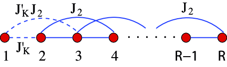
Figure 1: Schematic picture for the $J_{1}-J_{2}$ spin chain model (1.4) with an impurity located at the left boundary and coupled with $J_{K}^{\prime}$.

While unimportant for our analytic work, the spin chain representation, Eq. (1.4), dramatically alleviates the numerical work compared to using the Hamiltonian, Eq. (1.3). As discussed in A, the finite size corrections are much smaller when $J_{2}$ is fine-tuned to the critical point $J_{c}\approx.2412$ [56], a fact that, from a numerical perspective, presents a considerable advantage. For $J_{2}>J_{2}^{c}$ the spin chain enters a dimerized phase [57] with a gap and the relation between Eq. (1.4) and Kondo physics no longer holds. The two-fold degenerate dimerized ground-state is exactly known at the Majumdar-Ghosh [58] (MG) point, $J_{2}=J/2$, with the two ground-states corresponding to the two possible dimerization patterns. In the dimerized phase the fundamental excitations can be viewed as single $S=1/2$ solitons separating regions with these two distinct dimerization patterns. A sketch of the phase-diagram of the $J_{1}-J_{2}$ model summarizing these points is shown in Fig. 2.

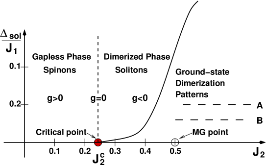
Figure 2: Phase diagram of the $J_{1}-J_{2}$ model as a function of $J_{2}$. The critical point $J_{2}^{c}\approx.2412$ separates a gapless Heisenberg phase from the dimerized phase. At the Majumdar-Ghosh (MG) point, $J_{2}=J_{1}/2$, the two exact ground-states, $A$ and $B$, for a system with an even number of spins are shown. For an odd number of spins a single spin (soliton) will separate regions with these two dimerization patterns.

At low energies, the spin chain model is equivalent to the Kondo model in any dimension, $D$. This is also true for the entanglement entropy as we show in B. A physical motivation for studying the Kondo model in the $D=2$-dimensional case is provided by the possibility of using the spins of gated semi-conductor quantum dots as qubits [59, 60, 61]. The various quantum dot spins would ideally be entangled only with each other. However, in practice, they would also be entangled with the surrounding conduction electrons which would cause limitations on the functioning of such a quantum computer [62, 53]. More generally, any physical realization of a quantum computer has a dissipative environment which is entangled, to some extent with the qubits. The Caldeira-Leggett (spin-boson) model [63] of a spin interacting with an ohmic dissipative environment is equivalent, at low energies to the Kondo model and entanglement in the Caldeira-Leggett model has been considered in recent work [62, 64]. The understanding of entanglement as it occurs in these quantum impurity models is therefore of considerable interest.

Spin chains have also been proposed for the purpose of creating quantum communication channels [65, 66, 67] and subsequent work has showed that entanglement in $S=1/2$ spin chain models can be used to establish perfect state transfer [68, 69, 70]. In most cases the couplings in the bulk of the chain are not uniform but vary with $r$, however, a model closely related to Eq. (1.4), where only the couplings at the end of the chain are modified have also been shown to accommodate perfect state transfer [71]. The algorithm for perfect state transfer proposed in [68] has been experimentally realized using a three-qubit liquid NMR quantum computer simulating a Heisenberg $XY$ interaction [72]. The possibility for using quantum spin chains as perfect quantum state mirrors has also recently been emphasized [73, 74]. From this perspective, entanglement in the spin chain model, Eq (1.4), is clearly of interest even aside from the relation to Kondo physics.

In the ground state of the Kondo model, the spin of the impurity is “screened” meaning that it effectively forms a singlet with the conduction electrons. This screening is expected to take place at an exponentially large length scale

$$\xi_{K}=v/T_{K}\propto e^{1/\lambda_{K}}.$$ (1.5)

Here $v$ is the velocity of the low energy excitations (fermions or spin-waves) and $T_{K}$, the Kondo temperature, is the energy scale at which the renormalized Kondo coupling becomes large. One of the interesting features of entanglement entropy in many body systems is its universality, which makes it useful for studying quantum phase transitions [3, 4, 5, 26]. A major conclusion of our work is that this universality extends to $S_{imp}$ in the following sense. When $\xi_{K}$ is large compared to all microscopic length scales in the system, and the system size $R$ is $\infty$, we find that $S_{imp}(r/\xi_{K})$ is a universal scaling function depending only on the ratio $r/\xi_{K}$. For finite systems of extent $R$ we find when $r,R-r,\xi_{K}\gg 1$:

$$S_{imp}\equiv S_{imp}(r/R,r/\xi_{K})$$ (1.6)

In this case, there are actually two different scaling functions depending on whether the total spin of the finite system ground state is $0$ or $1/2$. (For the spin chain these two cases correspond to $R$ even or odd respectively.) We emphasize that this holds for entanglement in both models Eq. (1.4) and (1.3). This extends to entanglement entropy the well-known universality of other properties of the Kondo model. We expect this universal scaling property to hold generally for quantum impurity models as was remarked on in [47]. An immediate consequence of this universality is that the same impurity entanglement entropy occurs, for large $r$, in many different microscopic models. It is insensitive, for example, to the dimensionality of space and the range of the Kondo interaction (as long as it is finite). In [75] preliminary density matrix group (DMRG) results obtained for the spin chain model, Eq. (1.4), at $J_{2}=J_{2}^{c}$ showed that the $r$-dependence of $S_{imp}$ confirms this picture and the presence of the length scale $\xi_{K}$ was demonstrated. In section 2 we provide additional evidence supporting this scaling at $J_{2}=J_{2}^{c}$ as well as results for for $J_{2}<J_{2}^{c}$.

The universal scaling functions are generally not amenable to analytic calculation except in certain limiting cases. The most straightforward of these is when $\xi_{K}\ll r$, in which case it is possible to perform calculations using Nozières local Fermi liquid theory (FLT) approach [76], as developed in [77, 78, 79]. In [75] initial analytical results using this approach were reported and in section 5 we present a detailed derivation and additional results notably at finite temperature.

When the Kondo coupling approaches either the weak coupling fixed point, $J_{K}^{\prime}=0$, or the strong coupling fixed point, $J_{K}^{\prime}=1$, one might have assumed that the impurity entanglement entropy would vanish. This turns out to be the case at the strong coupling fixed point, $J_{K}^{\prime}=1$. However, as we initially reported in [75], the impurity entanglement at the weak coupling fixed point is non-zero. In sections 2,7 we discuss in detail this fixed point entanglement entropy and further develop the intuitive picture for understanding it.

For $J_{2}>J_{2}^{c}$ the spin chain enters a dimerized phase [57] with a gap and the relation between Eq. (1.4) and Kondo physics no longer holds. However, entanglement as it occurs in spin chains without impurities, viewed as model systems for entanglement, is currently the focus of intense studies and is relatively well established both from a static [80, 81, 3, 82, 83, 26, 84, 85, 86, 87] and dynamic perspective [88, 89, 90]. Here we show that it is possible to obtain almost exact analytical results for the fixed point entanglement for the $J_{1}-J_{2}$ model, Eq. (1.4), in the dimerized phase. This approach is based on describing the lowest lying excitations in the dimerized phase as simple domain walls or single site solitons [91] which we refer to as thin solitons (TS) and is described in detail in section 6. While the use of gapped spin chains for the purpose of quantum communication and quantum computing is less evident than for gapless chains, the relative simplicity of the entanglement as it occurs in the dimerized phase allows for the development of an appealing intuitive picture of how the entanglement arises in terms of single particle entanglement (SPE) and impurity valence bonds (IVB). These concepts can be rigorously established using the TS approach in the dimerized phase and, more importantly, appear to be quite general concepts applicable to other models even in the absence of a gap. (See section 2).

The outline of the paper is as follows: In Section 2 we discuss in detail our definition of $S_{imp}$ and show additional evidence for the scaling behavior of Eq. (1.6) at $J_{2}=J_{2}^{c}$. The intuitive picture for understanding the impurity entanglement in terms of SPE and IVB is developed in Section 3 along with the fixed point entanglement. Weak scaling violations, related to another single-site measure for the impurity entanglement, $s_{imp}$, are discussed in Section 4. Section 5 contains a detailed account of the FLT approach for calculating $S_{imp}$ and Section 6 describe the thin soliton approach to performing variational calculations for the entanglement in the dimerized phase for $J_{2}>J_{2}^{c}$. Numerical results for the fixed point entanglement are presented in section 7. Most of the numerical results presented are density matrix renormalization group (DMRG) calculations performed on parallel SHARCnet computers keeping $m=256$ states. As we discuss in section 2 our working definition of $S_{imp}$ only focus on the uniform part of the entanglement. In section 8 we therefore present results for the alternating part of the entanglement as well as the dimerization. Finally we briefly summarize our main results in section 9.

This paper contains a number of appendices, some of which may be of quite general interest. In A we review field theory results on the $D$-dimensional Kondo model and the spin chain, and their relationship to each other. In B we extend these results to prove that the impurity entanglement entropy is the same for the $D$-dimensional Kondo model and the spin chain model. This appendix also contains a new derivation of the free fermion entanglement entropy in $D$-dimensions. In C we derive the 7-point formula used in the numerical work for extracting the uniform and alternating part of the entanglement entropy. In D we prove that the entanglement entropy is the same for all linear combinations of spin up and spin down elements of a doublet state. The connections between finite temperature entanglement entropy and thermal entropy are discussed in E. In F we present new results on the Majumdar-Ghosh model based on the thin soliton ansatz, including $\langle S^{z}_{r}\rangle$ in the ground state with open boundary conditions and an odd number of sites, and the dimerization, $\langle\vec{S}_{r}\cdot\vec{S}_{r+1}\rangle$.

2 The impurity Entanglement Entropy 

We begin by discussing our definition of the impurity entanglement entropy, Eq. (1.2). For impurity problems such as the Kondo model it is quite standard in experimental situations to define the impurity contribution to, for example, the susceptibility or the specific heat by subtracting reference values with the impurity absent. We have therefore defined the impurity entanglement analogously. For the $S=1/2$ spin chain the entanglement entropy has not only a uniform but also a staggered part [87]. For $r\gg 1$ we can write:

$$S(r,{R})=S_{U}(J^{\prime}_{K},r,{{R}})+(-1)^{r}S_{A}(J^{\prime}_{K},r,{{R}}),$$ (2.1)

where $S_{U}(J^{\prime}_{K},r,{{R}})$ and $S_{A}(J^{\prime}_{K},r,{{R}})$ are slowly varying functions or $r$. The entanglement entropy is also strongly dependent on whether the total spin of the ground-state of the system is $0$ or $1/2$, or, equivalently, whether $R$ is even or odd.

[In general, for ${R}$ odd, the ground state is a spin doublet. The entanglement entropy is the same for the spin up or down element of the doublet or for any linear combination of these states. We give a formal proof of this in D. The result follows from the fact that any linear combination of spin up and down can be obtained by a spin rotation from the spin up state. It is intuitively obvious that the entanglement entropy doesn’t depend on the direction of the spin quantization axis. For higher spin states the situation is more complex and in general different elements of the spin multiplet have different entanglement entropy.]

Theoretical work [2, 26] has established that for a uniform $S=1/2$ spin chain with periodic boundary conditions, or in general for gapless 1-D models, the entanglement entropy is given by:

$$S^{PBC}(r,{{R}})=\frac{c}{3}\ln\left[\frac{{R}}{\pi}\sin\left(\frac{\pi r}{{R}}\right)\right]+{s_{1}},$$ (2.2)

with $c=1$ and $s_{1}\simeq 0.726$ [92]. In this case there is no alternating term in the entanglement entropy. For the purpose of studying quantum impurity models, our focus is here exclusively on the case of an open $S=1/2$ spin chain where the alternating term, $S_{A}$, is non-zero [87] and it is known [26] that for a gapless system of linear extent $R$, the uniform part has a bulk part,

$$S_{U0}(r,{{R}})\approx\frac{1}{6}\ln\left[\frac{2{R}}{\pi}\sin\left(\frac{\pi r}{{R}}\right)\right]+\ln g+s_{1}/2,$$ (2.3)

independent of $J_{K}^{\prime}$, as well as an impurity contribution that will depend on $J_{K}^{\prime}$ and that is our main focus. Here $\ln g$ is the zero temperature thermodynamic impurity entropy [54]. We see that the presence of the boundary, in addition to generating an alternating term in $S$, have modified the uniform part of the entanglement entropy with respect to the result for periodic boundary conditions, Eq. (2.2). Note that both Eqs. (2.3) and Eq. (2.2) only are valid for critical models.

The impurity models we consider are defined using systems with open boundary conditions and when considering the impurity contribution to the entanglement care has to be taken with respect to the alternating term generated by the open boundary conditions. We do this by initially focusing only on the uniform part of the entanglement entropy and the contribution arising from the impurity to this part. Returning to our fundamental definition of $S_{imp}$, Eq. (1.2), we view $S$(no impurity) as the entanglement in a system without the impurity site, i.e. with one less site, $R-1$ and all couplings equal to unity. We do not define $S$(no impurity) as $S$ with $J_{K}^{\prime}=0$ since, as we shall discuss in detail later, for $J_{K}^{\prime}=0$ the impurity spin can have a non-trivial entanglement with the rest of the chain. It then follows that the complete impurity contribution to the entanglement entropy cannot be obtained by subtracting results for a system with $J_{K}^{\prime}=0$. We thus define the uniform part of the impurity entanglement entropy precisely as:

$$S_{imp}(J^{\prime}_{K},r,{{R}})\equiv S_{U}(J^{\prime}_{K},r,{{R}})-S_{U}(1,r-1,{{R}}-1),\ r>1.$$ (2.4)

For the subtracted part all couplings have unit strength. In a completely analogous manner one can also define the alternating part of the impurity entanglement entropy, $S_{imp}^{A}$, which we shall discuss in section 8 where it is shown that for $S^{A}_{imp}$ the scaling form is modified from that of Eq. (1.6). Our focus is therefore on the uniform part. For our numerical DMRG results a procedure for extracting the uniform and staggered part of the entanglement entropy is needed. We have found it sufficient to extract these functions by assuming that the uniform and staggered parts locally can be fitted by polynomials. If 7 sites surrounding the point of interest are used for the fitting a 7 point formula can easily be derived as outlined in C. The numerical work has been done using density matrix renormalization group [22] (DMRG) techniques in a fully parallelized version, keeping $m=256$ states. When performing calculations with $J_{K}^{\prime}=0$ and $R$ even we have found it necessary to use spin-inversion symmetry [93] under the DMRG iterations in order to select the desired singlet ground-state.

Other measures of the impurity entanglement entropy could have been defined and in section 4 we will discuss one of these, the single site entanglement of the impurity spin with the rest of the chain, $s_{imp}$. As we shall see, this quantity gives an incomplete picture of the impurity entanglement. Another possibility would be to define a relative entropy [16] between the state with the impurity and a reference state without the impurity. It would be interesting to explore this latter possibility. We expect that similar scaling would be found as we show here with our definition of $S_{imp}$.

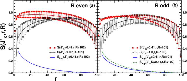
Figure 3: (a) DMRG results for the total entanglement entropy, $S(J^{\prime}_{K},r,R)$ for a 102 site spin chain at $J^{c}_{2}$, with a $J^{\prime}_{K}=0.41$ Kondo impurity ($\blacksquare$) along with $S(J^{\prime}_{K}=1,r-1,R-1)$ ($\square$). Uniform parts (solid lines) and the resulting $S_{imp}(J^{\prime}_{K}=0.41,r,R=102)$ for $R$ even. (b) DMRG results for the total entanglement entropy, $S(J^{\prime}_{K},r,R)$ for a 101 site spin chain at $J^{c}_{2}$, with a $J^{\prime}_{K}=0.41$ Kondo impurity ($\blacksquare$) along with $S(J^{\prime}_{K}=1,r-1,R-1)$ ($\square$). Uniform parts (solid lines) and the resulting $S_{imp}(J^{\prime}_{K}=0.41,r,R=101)$ for $R$ odd. For comparison we also show $S_{imp}(J^{\prime}_{K}=0.41,r,R=102)$ for $R$ even from panel (a) (dashed line).

To gain some insight into how the impurity influence the entanglement entropy and lead to a non-zero $S_{imp}$ we show in Fig. 3 data for $J_{K}^{\prime}=0.41$ for both $R$ even, Fig. 3(a) and $R$ odd, Fig. 3(b). There are significant differences between the results for $R$ even and $R$ odd. It is also clear that the influence of the impurity is felt more strongly for $R$ even compared to $R$ odd. The resulting $S_{imp}$ is clearly bigger for $R$ even for all $r$ as shown by the comparison in Fig. 3(b). In the limit where $J_{K}^{\prime}\to 0$ this difference becomes more pronounced since $S_{imp}$ for $R$ even increases with decreasing $J_{K}^{\prime}$ while for $R$ odd it tends to zero with decreasing $J_{K}^{\prime}$. For the value of $J_{K}^{\prime}=0.41$ used in Fig. 3 we shall later find that $\xi_{K}=25.65$ significantly smaller than $R$ and it would have been natural to expect features in $S_{imp}$ signaling the presence of this length scale. However, $S_{imp}$ is a monotonically decreasing function of $r$ for both parities of $R$ and no particular features are observed in $S_{imp}$ for $r$ of the order of $\xi_{K}$. It is important to note that this fact does not imply a violation of scaling of the form Eq. (1.6).

2.1 Scaling of $S_{imp}$ at $J_{2}^{c}$

The scaling of $S_{imp}(J_{K}^{\prime},r,{R})$ for fixed $r/{R}$ at $J_{2}=J_{2}^{c}$ was considered in detail in Ref. [75]. It was shown that $S_{imp}$ with $r/R$ fixed follows the expected scaling form, Eq. (1.6), and is a function of a single variable $r/\xi_{K}$. We expect this scaling to hold for $r,R-r,\xi_{K}\gg 1$ when the results are not influenced by microscopic parameters such as the lattice spacing. For the moderate system sizes of ${R}<102$ (${R}$ even) and ${R}<101$ (${R}$ odd) $S_{imp}$ shows a strong dependence on the parity of ${R}$ and two different scaling functions for ${R}$ even and odd were found. For $r/\xi_{K}\gg 1$ these two scaling functions are essentially the same but they differ significantly for $r/\xi_{K}\ll 1$. In the limit where ${R}\to\infty$ the two scaling functions eventually coincide. By requiring the data to collapse according to the scaling form, a naive estimate of $\xi_{K}$ can be obtained for both ${R}$ even and odd. In table 1 we list the resulting $\xi_{K}$ obtained through such an analysis.

$J^{\prime}_{K}$	0.8	0.6	0.525	0.45	0.41	0.37	0.30	0.25	0.225	0.20
$\xi_{K}$ ${R}$ even	1.89	5.58	9.30	17.40	25.65	40.5	111	299	$\sim$565	$\sim$1196
$\xi_{K}$ ${R}$ odd	1.65	5.45	9.30	17.40	25.65	39.2	127	411	$\sim$ 870	$\sim$ 2200

Table 1: The numerically determined values for $\xi_{K}(J_{K}^{\prime})$ using naive rescaling of $S_{imp}(J_{K}^{\prime},r,{R})$ at fixed $r/{R}$ for $J_{2}=J_{2}^{c}$. For ${R}$ odd system sizes of ${R}=19\ldots 101$ have been used and for ${R}$ even ${R}=18\ldots 102$. The estimates become unreliable once $\xi_{K}\gg{R}$.

We expect $S_{imp}$ to be a scaling function of only 2 parameters $S_{imp}(r/\xi_{K},r/{R})$, or, equivalently $S_{imp}(R/\xi_{K},r/{R})$ for $r,R,\xi_{K}\gg 1$. It should therefore also be possible to test this scaling by looking directly at $S_{imp}$ for fixed ${R}/\xi_{K}$ which should be a function of the single variable $r/{R}$. We use the previously determined $\xi_{K}$ listed in table 1 to test this assumption by selecting 2 sets of data, ${R}=400,J^{\prime}_{K}=0.41,\xi_{K}=25.65,{R}/\xi_{K}=15.59$ and ${R}=86,J^{\prime}_{K}=0.60,\xi_{K}=5.58,{R}/\xi_{K}=15.41$.

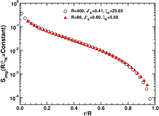
Figure 4: DMRG results for ${R}=400,J^{\prime}_{K}=0.41,\xi_{K}=25.65$ yielding ${R}/\xi_{K}=15.59$ (open circles) and ${R}=86,J^{\prime}_{K}=0.60,\xi_{K}=5.58$ with the ratio ${R}/\xi_{K}=15.41$ (full triangles) plotted versus $r/{R}$. $m=256$ states was kept in the DMRG calculation.

Our results are shown in Fig. 4 where we observe an excellent data collapse using the previously determined values of $\xi_{K}$ confirming the expected scaling form. Combined with the results presented in [75], this provides rather strong numerical evidence for the presence of the large length scale $\xi_{K}$ in the impurity entanglement entropy and demonstrates the scaling picture arising from the universal aspects of Kondo physics.

2.2 The Fixed Point Entanglement

It is instructive to consider what might be termed the fixed point entanglement, the entanglement occurring at the two fixed points at weak coupling $J_{K}^{\prime}=0$ and at strong coupling $J_{K}^{\prime}=1$. When $R$ is odd and $J^{\prime}_{K}=0$ the impurity spin is free while the remainder of the system is in a singlet ground-state. Due to the subtraction in Eq. (2.4) $S_{imp}$ as well as the alternating part $S^{A}_{imp}$ is then zero. Surprisingly, as was shown in [75], $S_{imp}(J^{\prime}_{K}=0,r,R)$ is non-zero when $R$ is even. We now discuss this in detail.

We consider the case ${R}$ even and the limit $J_{K}^{\prime}\to 0$. That is, out of the 4 degenerate states at $J_{K}^{\prime}=0$ we focus only on the singlet state, which is uniquely picked out by this limiting procedure. This state has a non-zero entanglement of the impurity spin with the rest of the system. On the other hand, to calculate the impurity entanglement entropy, defined in Eq. (2.4), we must subtract $S$ for a chain of odd length, ${R}-1$, with $J_{K}^{\prime}=1$. This odd length system has a spin doublet ground state. There is no simple relationship between $S(r,{R},J_{K}^{\prime}=0)$ and $S(r-1,{R}-1,J_{K}^{\prime}=1)$.

Explicitly, we may write the spin singlet ground state for a chain of even length ${R}$ in the form:

$$|\psi>=(1/\sqrt{2})[|\uparrow>|\Downarrow>-|\downarrow>|\Uparrow>].$$ (2.5)

Here the first arrow refers to the state of the impurity spin and the second, double arrow, to the total $S^{z}$ of all the other spins. We may write the pure state density matrix as:

$$\rho_{P}\equiv|\psi><\psi|=\frac{1}{2}\Big{[} |\uparrow><\uparrow|\otimes|\Downarrow><\Downarrow|+|\downarrow><\downarrow|\otimes|\Uparrow><\Uparrow|$$ (2.6)

$$-|\uparrow><\downarrow|\otimes|\Downarrow><\Uparrow|-|\downarrow><\uparrow|\otimes|\Uparrow><\Downarrow|\Big{]}.$$

Now consider doing the partial trace over the spins at sites $j$ with $r<j\leq R$. This trace can be done on each term separately in Eq. (2.6). It is convenient to define 4 operators on the Hilbert space of the $R-1$ spins $2,3,\ldots R$:

$$\rho_{m,m^{\prime}}\equiv\Tr_{B}|m><m^{\prime}|.$$ (2.7)

Here $m=\Uparrow$ or $\Downarrow$ (i.e. $\pm 1/2$). $\Tr_{B}$ means tracing over the spins at sites $j$ with $r<j\leq R$.

$$\rho_{\Downarrow\Uparrow}^{\dagger}=\rho_{\Uparrow\Downarrow}.$$ (2.8)

While $\rho_{\Downarrow\Downarrow}$ and $\rho_{\Uparrow\Uparrow}$ are themselves reduced density matrices for the $R-1$ site model, $\rho_{\Downarrow\Uparrow}$ is clearly not a reduced density matrix since it is not Hermitian. The two density matrices $\rho_{\Downarrow\Downarrow}$ and $\rho_{\Uparrow\Uparrow}$ are related by spin-inversion. The total reduced density matrix, including the impurity spin, can then be written:

$$\rho=\frac{1}{2}\left(\begin{array}[]{cc}\rho_{\Downarrow\Downarrow}&-\rho_{\Downarrow\Uparrow}\\ -\rho_{\Uparrow\Downarrow}&\rho_{\Uparrow\Uparrow}\end{array}\right).$$ (2.9)

When considering the fixed point impurity entanglement entropy $S_{imp}(J^{\prime}_{k}=0,r,R)$ the term we subtract in Eq. (2.4), the entanglement entropy for a chain of odd length $R-1$ with $J_{K}^{\prime}=1$, is given by $-Tr\rho_{\Uparrow\Uparrow}\log\rho_{\Uparrow\Uparrow}$ (or $-Tr\rho_{\Downarrow\Downarrow}\log\rho_{\Downarrow\Downarrow}$). Since, $\rho_{\Uparrow\Downarrow}$ is non-zero in the case at hand we see that $S_{imp}(J^{\prime}_{k}=0,r,R)$ is non-zero for $R$ even, also in the limit $R\to\infty$. The resulting $S_{imp}(J^{\prime}_{k}=0,r/R)$ was numerically calculated at $J_{2}^{c}$ in [75] using DMRG methods and was shown to crossover in an approximately linear manner from $\ln(2)$ at small $r/R$ to zero at $r/R=1$. We show additional results in section 7. This cross-over can be understood [75] in terms of a term corresponding to the zero temperature thermodynamic impurity entropy $\ln g$ shown to be present in the entanglement entropy at conformally invariant boundary fixed points [26].

If we now consider $S_{imp}(J^{\prime}_{K}=1,r/R)$ it will, up to a sign change, be the same for both $R$ even and $R$ odd since it is the difference in the uniform part of the entanglement entropy for an odd and even sized system. Since we expect the uniform part of the entanglement entropy to be independent of the parity of $R$ in the thermodynamic limit we expect $S_{imp}(J^{\prime}_{K}=1,r/R)$ to approach zero for increasing $R$ as was demonstrated numerically in [75]. We show additional results for $S_{imp}(J^{\prime}_{K}=1,r/R)$ at $J_{2}^{c}$ in section 7.

3 Impurity Valence Bonds (IVB) and Single Particle Entanglement (SPE)

In this section we define two heuristic quantities, the impurity valence bond (IVB) and the single particle entanglement (SPE). As we shall see these quantities capture essential parts of the impurity entanglement as described in the previous two sections. The IVB was first discussed in [75] and closely related ideas were developed by Refael and Moore in [94] (see also Ref. [95]). Here we recapitulate some of the results and further develop the ideas. In section 6 a much more complete development valid in the dimerized phase, $J_{2}>J_{2}^{c}$, showing more rigorously the presence of IVB and SPE terms in the entanglement entropy.

We start by discussing the single particle entanglement. We think in terms of a tight binding model describing a finite chain with a single particle present in a state where the particle has probability $p$ for being in region $A$ and $(1-p)$ for being in region $B$. The wave-function can quite generally be written $|\Psi\rangle=\sum_{i}\psi_{i}|i\rangle$, with $|i\rangle$ the coordinate space states, from which it follows that $p=\sum_{i\in A}|\psi_{i}|^{2}$. The reduced density matrix for region $A$ can then be written $p|1\rangle\langle 1|+(1-p)|0\rangle\langle 0|$ where $|1\rangle$ is the state with the particle in region $A$ and $|0\rangle$ the state with the particle in region $B$ (absent from $A$). It immediately follows that the entanglement entropy is given by:

$$S_{\rm SPE}=-p\ln p-(1-p)\ln(1-p).$$ (3.1)

We shall refer to this as the single particle entanglement contribution to the entanglement and we imagine that if a free spinon (or soliton) is present in the ground-state it should give rise to such a contribution to the uniform part of the entanglement entropy. Such a term would be present in the uniform part of the entanglement entropy for a uniform chain ($J^{\prime}_{K}=1$) for $R$ odd, where a single unpaired spin is present, but would likely be negligible for $R$ even at $J_{2}^{c}$. If we assume that the single spinon (soliton) picture is relevant at $J_{2}^{c}$ it follows that $S_{imp}(J^{\prime}_{k}=1,r/R)$ for $R$ odd should be given by the SPE. In [75] this was shown not to be the case but as we shall see it the SPE is a very good approximation in the dimerized phase and in particular at the Majumdar-Ghosh point.

The other component of the heuristic picture is the formation of an “impurity valence bond” (IVB) between the impurity and a site in the chain. See Fig. 5. When the IVB is cut by the boundary between regions $A$ and $B$ we expect it to give rise to a contribution of $\ln 2$ to the impurity part of the entanglement entropy. If the IVB does not cut this boundary the contribution to $S_{imp}$ arising from the IVB is zero. We then see that:

$$S_{imp}=(1-p)\ln 2,$$ (3.2)

where $p$ is the probability that the IVB connects the impurity spin to a site in region $A$. In the limit where $J_{k}^{\prime}\to 0$, the probability will, as above, be given by $p=\sum_{i\in A}|\psi_{i}|^{2}$ where $\psi_{i}$ now describe the wave-function of a single unpaired spin (soliton). At $J_{2}^{c}$ we expect the fixed point entanglement entropy $S_{imp}(J^{\prime}_{k}=0,r/R)$ for $R$ even to follow this form. In [75] this was shown to work well even at $J_{2}=J_{2}^{c}$. Care has to be given to the fact that the parity of $R$ will influence this picture and we now discuss the different situations in a preliminary manner, postponing a more complete discussion to section 6.

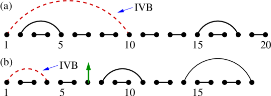
Figure 5: Typical impurity valence bond configurations for $R$ even (a) and $R$ odd (b). Note the unpaired spin on the $7^{\rm th}$ site in (b).

$R$ even and $J_{K}^{\prime}<1$: This situation is shown in Fig. 5(a). If $J_{K}^{\prime}=0$ we would expect the probability of forming an IVB between the impurity and a given site in the chain to be almost uniform throughout the chain. Hence, $S_{imp}$ should decrease approximately linearly with $r/R$ from $\ln 2$ to zero as mentioned above. For $J_{K}^{\prime}$ small but non-zero we expect the typical size of an IVB to be of the order of $\xi_{K}$ when $\xi_{K}<R$. In that case $S_{imp}$ should decrease monotonically to zero for $r/\xi_{K}\gg 1$. For $r/\xi_{K},r/R\ll 1$ we would expect it to approach $\ln 2$. This behavior is largely confirmed by the numerical DMRG calculations.

$R$ odd and $J_{K}^{\prime}<1$: This situation is shown in Fig. 5(b). Since $R$ is odd and the total spin of the system is $1/2$ there is an unpaired spin present in the ground-state. When $\xi_{K}\gg R$ the unpaired spin is the impurity spin and we simply have $S_{imp}=0$. As $\xi_{K}$ decreases the probability of creating an IVB increases due to screening of the impurity. However, the average length of the IVB when it is present decreases with $\xi_{K}$. In section 2.1 we showed clear numerical evidence for a monotonically decreasing $S_{imp}$ with $r$ for ${R}/\xi_{K}$ constant, however, if we instead now imagine keeping $r/R$ fixed and varying $R/\xi_{K}$ we see that the two above effects will trade off and give rise to a maximum in $S_{imp}$ for $\xi_{K}\approx R$ [75] with $R$ odd.

Eventually, in the limit $R\to\infty$, the parity of $R$ no longer plays a role and we obtain the same $S_{imp}(r/\xi_{K})$ for both $R$ even and $R$ odd. However, for mesoscopic systems these effects could be of importance.

3.1 The Entanglement entropy at the MG point

While the entanglement entropy at the critical point, $J_{2}^{c}$, is less amenable to the heuristic approach of this section, this intuitive picture sheds considerable light on the entanglement in the dimerized phase occurring for $J_{2}>J_{2}^{c}$ as we now discuss. In fact, almost exact expressions for the entanglement entropy can be obtained for the Majumdar Ghosh model. In section 6 we present a much more detailed approach based on a variational wave-function. At the MG point, the heuristic expression developed in this section for the entanglement entropy, follow directly from the variational approach.

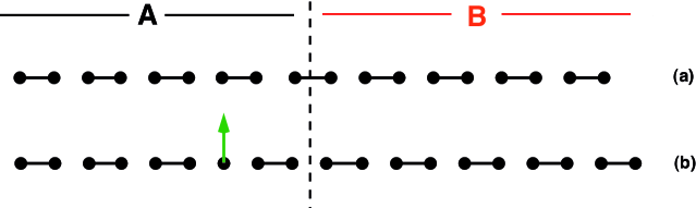
Figure 6: MG state divided in two regions $A$ and $B$. (a) The total number of site $R$ is even and the ground-state is a singlet. (b) When $R$ is odd, the ground-state contains a soliton ${\color[rgb]{0,1,0}\uparrow}$.

We now focus on the Majumdar-Ghosh model, $J_{2}=J/2$. Consider first the case $J_{K}^{\prime}=1$ and ${R}$ even. Then the ground state is a trivial nearest neighbor valence bond state on every link between sites $2i-1$ and $2i$, for $i=1,2,3\ldots{R}/2$, as depicted in Fig. 6 (a). When $r$ is even, $S=0$ since the ground state is a direct product of singlet states in regions $A$ and $B$. On the other hand, for $r$ odd, there is one valence bond, between sites $r$ and $r+1$, connecting regions $A$ and $B$. In this case $S=\ln 2$, as exemplified in Fig. 6 (a).

Now consider $J_{K}^{\prime}=1$ but ${R}$ odd. The ground state now contains one soliton (unpaired spin) on one of the odd sites. This soliton can be in region $A$ (see Fig. 6 (b)) with probability $p(r)$ or region $B$ with probability $1-p$, where:

$$p\equiv\sum_{n\in A}|\psi_{n}^{sol}|^{2},$$ (3.3)

and $\psi_{n}^{sol}$ describe the amplitude for the soliton to be on site $n$. The fact that regions $A$ and $B$ are sharing the soliton produces a “single particle entanglement” precisely as outlined above:

$$S_{SPE}=-p\ln p-(1-p)\ln(1-p).$$ (3.4)

However, this is not the whole story. We must also take into account that there may be a nearest neighbor valence bond connecting regions $A$ and $B$. Whether or not this is present depends both on the parity of $r$ and on whether the soliton is in region $A$ or $B$. If $r$ is even, then this valence bond is present when the soliton is in $A$. Conversely, if $r$ is odd, then it is present when the soliton is in region $B$. When this valence bond is present, it contributes an additional $\ln 2$ to $S$. The probability of it being present is $p$ for $r$ even and $1-p$ for $r$ odd. Adding this extra term we obtain:

$$S(r)=-p\ln p-(1-p)\ln(1-p)+[1/2+(-1)^{r}(p-1/2)]\ln 2.$$ (3.5)

As remarked earlier, when $J_{K}^{\prime}=0$ and ${R}$ is odd, the impurity site is unentangled with the rest of the chain which contains only nearest neighbor valence bonds, between sites $2i$ and $2i+1$. The only source of entanglement between $A$ and $B$ is a valence bond from site $r$ and $r+1$ when $r$ is even. Thus

$$S=(1/2)[1+(-1)^{r}]\ln 2.$$ (3.6)

Now, consider the case $J_{K}^{\prime}=0$ and ${R}$ even. Then there is an impurity valence bond stretching from site $1$ to some even site. All other valence bonds have length $1$. The right hand member of the impurity valence bond is again a soliton separating the $2$ different nearest neighbor valence bond ground states, but it now forms a singlet with the spin at site $1$. The soliton again contributes its single particle entanglement. Since the soliton forms a singlet with site $1$ this contributes $\ln 2$ to $S$ when the IVB terminates in region $B$, with probability $[1-p(r)]$ but make no contribution when it terminates in region $A$. Furthermore, there may be an additional nearest neighbor valence bond entangling regions $A$ and $B$ and contributing another $\ln 2$ to $S$. When $r$ is even, this occurs when the IVB terminates in region $B$, with probability $(1-p)$. When $r$ is odd it occurs when the IVB terminates in region $A$, with probability $p$. Combining the contributions of the SPE, the IVB and the possible nearest neighbor valence bond gives:

$$S=-p\ln p-(1-p)\ln(1-p)+[3/2-p+(-1)^{r}(1/2-p)]\ln 2.$$ (3.7)

Both Eqs (3.7) and (3.5) are shown to agree very well with numerical results at the MG-point presented in section 7.

4 $s_{imp}$ and Weak Scaling Violations 

The simplest measure of how a qubit is entangled with the environment would be to take system $A$ to be the impurity spin (qubit) itself and regard the environment as region $B$ [53]. Often this is referred to as single site entanglement. If system $A$ only contains the single impurity spin at the boundary of the chain it becomes impossible to extract the uniform part and we can therefore not use Eq. (2.4) to define the impurity entanglement. Instead we have to use the complete entanglement entropy including both uniform and alternating parts. To distinguish it from $S_{imp}$ in Eq. (2.4) we therefore denote it by $s_{imp}$ and define it as $S(J_{K}^{\prime},1,{R})$ with no subtraction. We now analyze this quantity.

First consider the case of ${R}$ even. Then the ground state is a spin singlet. Since the impurity has spin-1/2, as does the rest of the system, we can write the spin-zero ground state in the form:

$$|\psi>=(1/\sqrt{2})[|\uparrow>\otimes|\Downarrow>-|\downarrow>\otimes|\Uparrow>],$$ (4.1)

where the single arrow labels the state of the impurity and the double arrow the state of the rest of the system. Tracing out the rest of the system gives a two-dimensional density matrix for the impurity spin which is diagonal with elements $1/2$ and hence a maximal entanglement entropy of $\ln 2$. The case of odd ${R}$ is more interesting. Now the ground state is a doublet with total spin $S_{T}=1/2$. Let us focus on the state with $S^{z}_{T}=+1/2$. This must have the form:

$$|\psi>=a|\uparrow>\otimes|0,0>+b|\downarrow>\otimes|0,1>,$$ (4.2)

where $|0,0>$ denotes a spin singlet state of the rest of the system and $|1,1>$ denotes an $S=1$, $S^{z}=1$ state of the rest of the system. All states are normalized to $1$, so it follows that $|a|^{2}+|b|^{2}=1$. The density matrix is again diagonal with matrix elements $|a|^{2}$ and $|b|^{2}$ and hence

$$s_{imp}=-|a|^{2}\ln|a|^{2}-|b|^{2}\ln|b|^{2}.$$ (4.3)

On the other hand, the magnetization of the impurity in the ground states is given by:

$$m_{imp}=(|a|^{2}-|b|^{2})/2=(2|a|^{2}-1)/2.$$ (4.4)

Thus we may write:

$$s_{imp}=-\sum_{\pm}(1/2\pm m_{imp})\ln[(1/2\pm m_{imp})].$$ (4.5)

(This formula is also trivially true for the case ${R}$ even in which case $m_{imp}=0$.) For ${R}$ odd, $m_{imp}$, and hence $s_{imp}$, shows an interesting dependence on ${R}$ which reflects Kondo physics. $m_{imp}$ was studied, for the usual fermion Kondo model, in [96] and [97, 98] for example. For weak Kondo coupling and relatively short chains, ${R}\ll\xi_{K}$, $m_{imp}\approx 1/2$. On the other hand, for stronger Kondo coupling or larger chains, the magnetization is progressively transferred from the impurity to the rest of the chain, associated with screening of the impurity. In the limit of an infinite bare Kondo coupling, $m_{imp}=0$ since the impurity spin then forms a singlet with one other electron and all of the magnetization resides in the other electrons, which have individual magnetization of order $1/{R}$.

Nonetheless, $m_{imp}$ is not a scaling function of ${R}/\xi_{K}$. This is associated with the fact that the operator $\vec{S}_{imp}$ has an anomalous dimension[97, 98], $\gamma_{imp}(\lambda_{K})$. Thus it obeys the renormalization group equation:

$$\left[{R}\frac{\partial}{\partial{R}}+\beta(\lambda_{K})\frac{\partial}{\partial\ \lambda_{K}}+\gamma_{imp}(\lambda_{K})\right]m_{imp}({R},\lambda_{K})=0.$$ (4.6)

The weak coupling $\beta$-function, the variation of the effective Kondo coupling as we vary the length scale is:

$$\frac{d\lambda_{K}}{d\ln L}=-\beta(\lambda_{K})=\lambda_{K}^{2}-\frac{1}{2}\lambda_{K}^{3}+\ldots$$ (4.7)

We then see that if $\gamma_{imp}(\lambda_{K})$ were zero, (4.6) would imply that $m_{imp}$ was a function of $\lambda_{eff}({R})$ only, or equivalently a function of $\xi_{K}/{R}$ only. However, a non-zero $\gamma_{imp}\neq 0$, as occurs here, implies scaling violations. At lowest non-vanishing order [99, 97, 98] in $\lambda_{K}$,

$$\gamma_{imp}(\lambda_{K})=\lambda_{K}^{2}/2+\ldots$$ (4.8)

The general solution of (4.6) is:

$$m_{imp}=\exp\{\int_{0}^{\lambda_{K}^{0}}[\gamma(\lambda_{K})/\beta(\lambda_{K})]d\lambda_{K}\}f(\xi_{K}/{R}),$$ (4.9)

where $f$ is some function of $\xi_{K}/{R}$ or equivalently of $\lambda_{K}({R})$. From (4.7) and (4.8) we see that

$$\exp\{\int_{0}^{\lambda_{K}^{0}}[\gamma(\lambda_{K})/\beta(\lambda_{K})]d\lambda_{K}\}=1+\lambda_{K}^{0}/2+O[(\lambda_{K}^{0})^{2}].$$ (4.10)

The fact that $m_{imp}$ has this residual dependence on the bare coupling which cannot be adsorbed into the renormalized coupling at scale ${R}$ implies a violation of scaling. However, since this effect vanishes as the bare coupling, $\lambda_{K}^{0}\to 0$, we refer to it as a “weak scaling violation”.

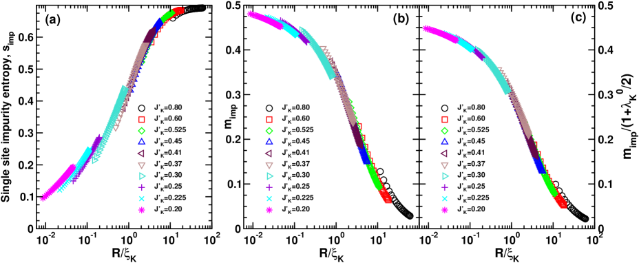
Figure 7: (a) Weak scaling violations for the single site impurity entanglement entropy $s_{imp}$ (a) [Eq. (4.5)] and the local impurity magnetization $m_{imp}=\langle S_{1}^{z}\rangle$ (b). In panel (c) is shown an improved scaling plot of $m_{imp}/(1+\lambda_{K}^{0}/2)$. The $\xi_{K}$ used in all panels are from table 1. All data are for odd length chains between $R=19\ldots 101$.

This form of $m_{imp}$, exhibiting weak scaling violation, can be confirmed by an explicit perturbative calculation. This calculation was actually presented earlier in [96] for the 1D lattice version of the fermionic Kondo Hamiltonian:

$$H=-t\sum_{j=1}^{{R}-2}(\psi_{j}^{\dagger}\psi_{j+1}+h.c.)+J_{K}\vec{S}_{imp}\cdot\psi^{\dagger}_{1}\frac{\vec{\sigma}}{2}\psi_{1}.$$ (4.11)

In [96] ${R}-1$ was called $L$. The result was:

$$m_{imp}=\frac{1}{2}-\left[\frac{J_{K}}{(L+1)}\right]^{2}\sum_{k,k^{\prime}}\theta(\epsilon_{k^{\prime}})\theta(-\epsilon_{k})\left[\frac{\sin k\sin k^{\prime}}{\epsilon_{k}-\epsilon_{k^{\prime}}}\right]^{2}.$$ (4.12)

Here $\theta(x)$ is the Heavyside or step function, and $\epsilon_{k}=-2t\cos k$ is the dispersion relation. The allowed values of $k$ and $k^{\prime}$ occurring in the sum in (4.12) are $k=\pi n/{R}$ for $n=1,2,3,\ldots$. Assuming ${R}\gg 1$, we replace the sums by integrals. The integrals diverge logarithmically at $k=k^{\prime}=k_{F}=\pi/2$. Letting $k=\pi/2-q$ and $k^{\prime}=\pi/2-q^{\prime}$, the integrals near $q,q^{\prime}=0$ take the form:

$$m_{imp} \approx \frac{1}{2}-\left[\frac{J_{K}}{\pi v}\right]^{2}\int_{0}^{\infty}dq\int_{0}^{\infty}dq^{\prime}\frac{1}{(q+q^{\prime})^{2}}$$ (4.13)

$$\approx \frac{1}{2}-\left[\frac{J_{K}}{\pi v}\right]^{2}\int_{0}^{\infty}\frac{dq}{q}$$

$$\approx \frac{1}{2}-\left[\frac{J_{K}}{\pi v}\right]^{2}\ln({R}/a).$$

Here we have replaced the small $q$ limit of the integral by $1/{R}$ and the large $q$ limit by a short distance cut off, $a$, of order a lattice spacing. The continuum limit of this tight binding model gives the Hamiltonian of (1.3) with $\lambda_{K}=J_{K}/\pi t$ and $v=2t$, so we may write this as:

$$m_{imp}\approx\frac{1}{2}-\left[\frac{\lambda_{K}^{0}}{2}\right]^{2}\ln({R}/a).$$ (4.14)

The lowest order correction to the effective coupling as determined by the first (quadratic) term in the $\beta$-function is:

$$\lambda_{K}({R})\approx\lambda_{K}^{0}+(\lambda_{K}^{0})^{2}\ln({R}/a^{\prime})+\ldots,$$ (4.15)

where $a^{\prime}$ is another short distance cut off. Thus we see that, to $O[(\lambda_{K}^{0})^{2}]$ we can write:

$$m_{imp} \approx \left[1+\frac{\lambda_{K}^{0}}{2}\right]\left[\frac{1}{2}-\frac{\lambda_{K}^{0}}{4}-\frac{(\lambda_{K}^{0})^{2}}{4}\ln({R}/a^{\prime})\right]$$ (4.16)

$$\left[1+\frac{\lambda_{K}^{0}}{2}\right]\left[\frac{1}{2}-\frac{\lambda_{K}({R})}{4}\right].$$

This has the form of (4.9) with the scaling function:

$$f[\lambda_{K}({R})]\approx\frac{1}{2}-\frac{\lambda_{K}({R})}{4}+\ldots\approx\frac{1}{2}-\frac{1}{4\ln({R}/\xi_{K})}+\ldots.$$ (4.17)

The $\ldots$ represents terms of $O(\lambda_{K}(R)^{2}$ and higher in the effective coupling at scale ${R}$.

The fact that $m_{imp}$ exhibits weak scaling violations implies that $s_{imp}$ does also, as displayed in Figs. 7(a). In Fig. 7 we show DMRG results obtained at the critical point $J_{2}=0.2412$ for various odd lengths $19\leq{R}\leq 101$ and Kondo couplings $0.2\leq J^{\prime}_{K}\leq 0.8$. The local magnetization at the impurity site $m_{imp}=\langle S_{1}^{z}\rangle$ is shown in Fig. 7(b) as a function of ${R}/\xi_{K}$, using the values of $\xi_{K}(J^{\prime}_{K})$ determined previously (table 1). Clearly both $s_{imp}$ and $m_{imp}$ violate scaling since the various curves do not fall on top of each other. As outlined above we expect $m_{imp}/(1+\lambda_{K}^{0}/2)$ to scale much better and this is shown in Fig 7(c). Some deviations from scaling are still visible but clearly the scaling has improved. We expect the remaining discrepancies could be improved upon by using more optimal values for $\xi_{K}$ instead of the ones determined from other scaling plots which have significant uncertainties associated with them for either very large or very small $\xi_{K}$.

The Kondo physics also is expected for $J_{2}\leq J_{2}^{c}$ and therefore also for the unfrustrated chain at $J_{2}=0$ [55]. The unfrustrated spin chain model can be investigated using Quantum Monte Carlo (QMC) methods as an alternative to the DMRG computations. Since QMC works for any temperature, it allows to investigate finite temperature scaling properties like the spin susceptibility (see Ref. [55]) from where we can get precise estimates for the Kondo temperature $T_{K}=v_{s}/\xi_{K}$. These estimates, given in table 2 (along with estimates obtained in Ref. [55] by solving the Bethe Ansatz equations for this model [100]), are then used to check the scaling violations at $J_{2}=0$ of the local magnetization at the impurity site as well as the single site impurity entanglement entropy. As in the frustrated case discussed above, also here the weak scaling violations are clearly present. In Fig. 8, we show the QMC results obtained for various odd lengths $9\leq{R}\leq 257$ and Kondo couplings $0.1\leq J^{\prime}_{K}\leq 0.8$ where $m_{imp}$ violates scaling as well as $s_{imp}$.

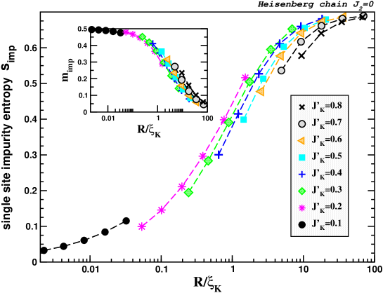
Figure 8: Weak scaling violations for the local impurity magnetization $m_{imp}=\langle S_{1}^{z}\rangle$ (inset) and the single site impurity entanglement entropy $s_{imp}$ [Eq. (4.5)] (main panel). QMC results obtained for the critical spin chain [model (1.4)] at $J_{2}=0$ with various odd lengths ${R}$ and Kondo couplings $J^{\prime}_{K}$ indicated on the plot. The scaling violations are shown as a clear non-universality as a function of ${R}/\xi_{K}(J^{\prime}_{K})$

$J^{\prime}_{K}$	$0.1$	$0.2$	$0.3$	$0.4$	$0.5$	$0.6$	$0.7$	$0.8$
$\xi_{K}$	$\sim 4\times 10^{3}$	$168$	$37$	$14$	$6.24$	$3.5$	$1.8$	$0.95$

Table 2: $\xi_{K}(J_{K}^{\prime})$ for $J_{2}=0$, as determined from scaling of the finite temperature impurity susceptibility and Bethe Ansatz calculations (reported in Ref. [55]).

4.1 Discussion

In [97, 98] a rather general discussion was given of which physical quantities are given by pure scaling functions and which ones exhibit weak scaling violations. In general quantities defined far from the impurity, such as the local susceptibility, are pure scaling functions whereas those that depend explicitly on the impurity spin operator exhibit weak scaling violations. In particular, the impurity susceptibility and specific heat or (thermodynamic) entropy are given by pure scaling functions. This is because they only involve conserved quantities, the total spin and Hamiltonian operators which have zero anomalous dimension. (Roughly speaking, for the case of the total spin operator, the anomalous dimension of the impurity spin operator is canceled by the anomalous dimension of the electron spin density operator near the impurity.) We expect the impurity entanglement entropy, $S_{imp}(J_{K}^{\prime},r,{R})$ to be a pure scaling function when $r\gg 1$, since it is a quantity defined far from the impurity. Indeed, in the approach of Cardy and Calabrese, reviewed in Sec. 5 the entanglement entropy is obtained from Green’s functions of an operator $\Phi_{n}$, which is inserted at the positions $\pm r$. Since this operator is inserted at a location far from the boundary, we expect that it will not have any anomalous dimension associated with the Kondo interaction. Therefore the one-point function obeys the RG equation of Eq. (4.6) with zero anomalous dimension, implying that it is a pure scaling function. Indeed our DMRG data is consistent with such scaling behavior as we have shown in Fig. (4).

5 Fermi Liquid Theory for $S_{imp}$ 

In the limit $\xi_{K}\ll r$, within the FLT as outlined in A, we can also calculate $S_{imp}$ by treating $H_{int}$ in Eq. (1.17) in lowest order perturbation theory. The entanglement entropy is obtained by means of the replica trick. If Tr$\rho(r)^{n}$ is known,

$$S=-\lim_{n\to 1}\frac{d}{dn}[{\rm Tr}\rho(r)^{n}],$$ (5.1)

where $\rho(r)$ is the reduced density matrix for the subsystem $(0,r)$. In the path integral representation of Euclidean space-time,

$${\rm Tr}\rho(r)^{n}=\frac{Z_{n}(r)}{Z^{n}},$$ (5.2)

where $Z_{n}(r)$ is the partition function on an $n$-sheeted Riemann surface ${\cal R}_{n}$, with the sheets joined at the cut extending from $r$ to ${R}$ [2, 26]. Now the original problem has been transformed into the calculation of the partition function with a nontrivial geometry. We use the approach where the Hamiltonian is written in terms of left movers only, obeying PBC on an interval of length $2{R}$. (See A). In the critical region, the system is conformally invariant and CFT methods are applicable. Starting with zero temperature, the $n$-sheeted Riemann surface ${\cal R}_{n}$, can be mapped to the usual complex plane ${\cal C}$ [26]. Then the expectation value of the energy momentum tensor $T$ on ${\cal R}_{n}$ is simply given by the Schwartzian derivative:

$$\langle T(w)\rangle_{\mathcal{R}_{n}}=\frac{\Delta_{n}(u_{1}-u_{2})^{2}}{(w-u_{1})^{2}(w-u_{2})^{2}},$$ (5.3)

where $\Delta_{n}=(c/24)(1-(1/n)^{2})$ and we have $u_{1}=ir$ and $u_{2}=-ir$ here. Then Calabrese and Cardy [26] observed its important connection to the correlators on ${\cal C}$ through the Ward identity:

$$\left\langle T(w)\right\rangle_{{\cal R}_{n}} \equiv \frac{\int[d\phi]T(w)e^{-S_{E}({\cal R}_{n})}}{\int[d\phi]e^{-S_{E}({\cal R}_{n})}}$$ (5.4)

$$= \frac{\left\langle T(w)\Phi_{n}(r)\Phi_{-n}(-r)\right\rangle_{{\cal C}}}{\left\langle\Phi_{n}(r)\Phi_{-n}(-r)\right\rangle_{{\cal C}}}.$$

The fictitious primary operators $\Phi_{\pm n}$ on the branch points have the left scaling dimensions $\Delta_{n}$. They concluded that Tr$\rho^{n}=$ $Z_{n}/Z^{n}$ behave identically to the $n$-th power of $\left\langle\Phi_{n}(r)\Phi_{-n}(-r)\right\rangle_{{\cal C}}$ under the conformal mappings or explicitly,

$${\rm Tr}\rho^{n}\cong\tilde{c}_{n}(2r/a)^{(c/12)(n-1/n)}.$$ (5.5)

Applying the replica trick, the entanglement entropy is $S\sim(c/6)\ln(2r)$. Then they extended the result to finite system size ${R}$ or infinite system size and finite temperature $T=1/\beta$ by applying the corresponding conformal mapping to $\left\langle\Phi_{n}(r)\Phi_{-n}(-r)\right\rangle_{{\cal C}}$ [26].

Now with the presence of the local irrelevant interaction Eq. (1.17), we should calculate perturbatively the correction to the partition function $Z_{n}$ in order to get the impurity entanglement entropy $S_{imp}$. Luckily, the irrelevant interaction is just the energy momentum tensor itself and its expectation value on the $n$-sheeted Riemann surface is just Eq. (5.3). The correction to $Z_{n}$ of first order in $\xi_{K}$ is:

$$-\delta Z_{n}=-(\xi_{K}\pi)n\int_{-\infty}^{\infty}d\tau\langle{\cal H}_{s,L}(\tau,0)\rangle_{{\cal R}_{n}}.$$ (5.6)

${\cal H}_{s,L}=T/(2\pi)$ where $T(\tau,x)$ is the conventionally normalized energy-momentum tensor for the $c=1$, free boson conformal field theory corresponding to the spin excitations of the original free fermion model. After doing the simple integral and taking the replica limit, for ${R}\rightarrow\infty$, we get

$$S_{imp}=\pi\xi_{K}/(12r).$$ (5.7)

In principle, in order to extend the FLT calculation to finite ${R}$, we will need the conformal mapping from a infinite $n$-sheeted Riemann surface to a finite one. On the other hand, we can also try to exploit Eq. (5.4) following ideas similar to Ref. [26] by applying the standard finite size conformal mapping to both $\left\langle T\Phi_{n}\Phi_{-n}\right\rangle_{{\cal C}}$ and $\left\langle\Phi_{n}\Phi_{-n}\right\rangle_{{\cal C}}$. Then, in the first order perturbation,

$$-\delta(\frac{Z_{n}}{Z^{n}})=-(\frac{\xi_{K}}{2})n\int_{-\infty}^{\infty}d\tau[(\frac{\pi}{2{R}})\frac{\sinh[i\pi r/({R})]}{\sinh[\frac{\pi(v\tau+ir)}{2{R}}]\sinh[\frac{\pi(v\tau-ir)}{2{R}}]}]^{2}.$$ (5.8)

We use the integral

$$\int_{0}^{\infty}\frac{dx}{\cosh ax-\cos t}=\frac{t}{a}\csc t,$$ (5.9)

from Ref. [101] and differentiate Eq. (5.9) with respect to $t$ on the both sides. Applying this result and the product-to-sum hyperbolic identity to Eq. (5.8), we can complete the integral and after the replica limit we get:

$$S_{imp}=\frac{\pi\xi_{K}}{12{R}}[1+\pi(1-\frac{r}{{R}})\cot(\frac{\pi r}{{R}})].$$ (5.10)

Of course, Eq. (5.10) reduces to Eq. (5.7) for ${R}$ $\gg r$ and both of them agree with the scaling form of $S_{imp}$. Interestingly, Eq. (5.10) can be regarded as the first order Taylor expansion in $\xi_{K}/r$ and $\xi_{K}/{R}$ of $S_{U}=(1/6)\ln[{R}\sin\pi r/{R}]$ with $r$ and ${R}$ both shifted by $\pi\xi_{K}/2$. Consistently, Eq. (5.7) can also be obtained from expanding $(1/6)\ln(r+\pi\xi_{K}/2)$. In fact, many other quantities such as impurity susceptibility, specific heat and ground state energy correction can be also obtained in this fashion by shifting the size of the total system, ${R}$, to ${R}+\pi\xi_{K}/2.$

Within CFT methods, we can also calculate $S_{imp}$ for infinite ${R}$ but at finite temperature $\beta$. We apply the standard finite temperature conformal mapping to $\left\langle T\Phi_{n}\Phi_{-n}\right\rangle_{{\cal C}}$ and $\left\langle\Phi_{n}\Phi_{-n}\right\rangle_{{\cal C}}$. The result for first order perturbation is just to replace $2{R}$ by $\beta$ and sinh by sin in Eq. (5.8) with the integral from $-\beta/2$ to $\beta/2$. Completing the straightforward integral yields

$$S_{imp}=[\pi^{2}\xi_{K}T/(6v)]\coth(2\pi rT/v),$$ (5.11)

valid for $T,v/r\ll T_{K}$. In the intermediate temperature regime, $v/r\ll T\ll T_{K}$ and hence $rT\gg v$, Eq. (5.11) approaches the thermodynamic impurity entropy, $S_{imp}\to\pi^{2}\xi_{K}T/(6v)=\pi^{2}T/(6T_{K})=c_{imp}(T)$, the well-known impurity specific heat. ($T_{K}\equiv v/\xi_{K}$ is the Kondo temperature.) This is consistent with the observation that in this limit the entanglement entropy approaches the thermodynamic entropy as noted in Ref. [26]. In E this connection is explored in more detail and it is argued that quite generally $S$ will approach the thermodynamic entropy for $T\gg v/r$.

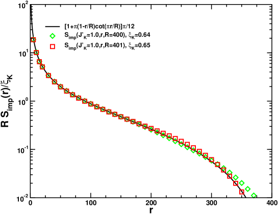
Figure 9: $S_{imp}(J^{\prime}_{K}=1,r,{R})$ for ${R}=400,401$ compared to the FLT prediction, Eq. (5.10).

The FLT expression for the uniform part of the entanglement entropy, Eq. (5.10) has been compared in detail with numerical DMRG data in Ref. [75]. The resulting values for $\xi_{K}$ are shown in table 3. Excellent agreement between this expression and numerical data for $S_{imp}(J^{\prime}_{K},r,{R})$ was found for $J_{K}^{\prime}\lesssim 1$. However, the fixed point impurity entanglement entropy $S_{imp}(J^{\prime}_{K}=1,r,{R})$ with $J_{K}^{\prime}=1$ itself should in fact be given by this same expression for ${R}$ both even and odd. Now, with a $\xi_{K}=0.65$ of order ${}(1)$. In Fig. 9 we show results for $S_{imp}(J^{\prime}_{K}=1,r,{R})$ for ${R}=400,401$. In both cases do we find good agreement with the FLT result, Eq. (5.10). The small discrepancies between the numerical data and the FLT results for $r$ close to 400 are likely due to the approximate forms used for extracting the uniform and alternating parts of the numerical data. For $J_{K}^{\prime}\neq 1$ these discrepancies are less pronounced since the numerical signal for $S_{imp}$ is larger by a factor of ${R}/\xi_{K}$.

It is important to note that the observed agreement implies that the fixed point impurity entanglement entropy, $S_{imp}(J_{K}^{\prime}=1,r,{R})\sim 1/{R}$ for both even and odd $R$ and hence is zero in the thermodynamic limit.

$J^{\prime}_{K}$	1.00	0.80	0.60	0.525	0.45	0.41	0.37	0.30
$\xi_{K}$	0.65	1.97	5.93	9.84	17.83	25.65	38.29	83.79

Table 3: $\xi_{K}(J_{K}^{\prime})$ as determined from $S_{imp}(J_{K}^{\prime},r,{R})$ for ${R}=400$ using the FLT prediction, Eq. (5.10). The estimates become unreliable once $\xi_{K}$ becomes comparable to ${R}$.

6 The TS- and OTS-ansatz for the Dimerized Phase, $J_{2}^{c}<J_{2}\leq J/2$

For $J_{2}>J_{2}^{c}$ the spin chain model, Eq. (1.4), develops a gap and a non-zero dimerization. The well known Majumdar-Ghosh (MG) model [58] ($J_{2}=J/2$) is part of this phase and we therefore take the MG model as our starting point for an analysis of the entanglement entropy in the dimerized phase. The MG point constitutes a disorder point [102] beyond which the short-range correlations become incommensurate and our analysis therefore focus on the regime $J_{2}^{c}\leq J_{2}<J/2$. Due to the gap above the dimerized ground-state, it becomes possible to proceed using variational wavefunctions for this range of parameters, yielding surprisingly precise results. The initial assumption is that the lowest excitation in the dimerized phase is described by a single free spin acting as domain wall or a soliton. This is an approximation since a complete description would include states where the domain wall extends over several sites. The thin soliton states are not orthonormal. By assuming that they are, we arrive at a further simplified ansatz which never the less proves to be surprisingly precise. Below we detail this approach.

6.1 The Thin Soliton (TS) Ansatz

For the MG model [58] ($J_{2}=J/2$) it is well known that for ${R}$ even the singlet ground-state is two fold degenerate [58, 91, 103, 104]. These two ground-states corresponds to the formation of singlet states between nearest neighbor spins either between sites $2n+1$ and $2n+2$ or $2n+2$ and $2n+3$. The resulting dimerization then occurs in two distinct patterns. (See Fig. 6.) For ${R}$ odd a very good approximation to the ground-state is obtained by assuming that a single spin, the soliton, is left unpaired separating regions with dimerizations in the two above mentioned patterns. If we number the sites of the system $r=1,\ldots,{R}$ the number of odd sites is given by $N^{o}=({R}+1)/2$. We define a state $|n\rangle$ by:

$$|n\rangle\equiv|\overbrace{-\ \ldots\ -}^{n}\ \uparrow\ -\ \ldots\ -\rangle.$$ (6.1)

Here, $-$ indicates a singlet between site $r$ and $r+1$ with $n=0,\ldots N_{d}=N^{o}-1$ such singlets occurring before the soliton indicated by the $\uparrow$. Here, $n$ can take on the values $n=0,\ldots N_{d}=N^{o}-1$ with $N_{d}$ the total number of dimers. Note that, singlets to the left of the soliton occur between sites $[2n+1,2n+2]$ and between sites $[2n+2,2n+3]$ to the right of the soliton. We use the Marshall sign convention that $[2n+1,2n+2]=(|\uparrow\downarrow\rangle-|\downarrow\uparrow\rangle)/\sqrt{2}$ whereas $[2n+2,2n+3]=(|\downarrow\uparrow\rangle-|\uparrow\downarrow\rangle)/\sqrt{2}$. We shall refer to these states as thin soliton states (TS-states) since the soliton is not “spread” out over several sites by including valence bonds of more than unit length. Note that, in such a dimerized state the soliton can, for ${R}$ odd, only be situated on odd sites $r=1,3,5,\ldots{R}$. We can then write an ansatz for the ground-state wavefunction in the following manner [91, 103, 104, 105]:

$$|\Psi_{TS}^{\Uparrow}\rangle\simeq\sum_{n=0}^{N_{d}}\psi^{sol}_{n}|n\rangle.$$ (6.2)

We shall refer to this ansatz as the thin-soliton ansatz (TS-ansatz). If we consider ${R}=5$, we find 3 linearly independent (but not orthogonal) thin soliton states. However, with 5 $S=1/2$ spins it is easy to see that there are in fact 5 $S=1/2$ states. The thin soliton states do therefore not form a complete basis for the $S=1/2$ subspace and the TS-ansatz is therefore variational in nature for ${R}$ odd. However, for the MG-model it is known that the TS-ansatz is very precise [103, 104, 105]. Caspers et al [103, 104] improved on the TS-ansatz by including terms with longer valence bonds in a systematic manner and showed that the resulting variational energies were only changed slightly.

For ${R}$ even Shastry and Sutherland [91] considered excited states corresponding to 2-soliton states and studied bound-states of solitons with relatively high energies. Subsequently, exact wave-functions for bound soliton states were found by Caspers and Magnus [103]. However, at low energies the solitons behave as free massive particles [105] with the soliton mass defined by:

$$\Delta_{sol}=\lim_{{R}\to\infty}E({R})-\frac{E({R}+1)+E({R}-1)}{2},\ \ {R}\ \mathrm{odd}.$$ (6.3)

Here $E(R)$ is the ground-state energy for a system of length $R$. Using DMRG the mass of the soliton has been estimated [105] for the MG model:

$$\Delta_{sol}^{DMRG}/J=0.1170(2).$$ (6.4)

Using the TS-ansatz and periodic boundary conditions (pbc) the soliton mass was determined to be [103, 104] $\Delta_{sol}^{TS,pbc}/J=0.125$ and including 3 and 5 spin structures in the variational calculation [103, 104] the estimate improved to $0.11701$. Note that the ground-state energy, $E(R)$, is an extensive quantity and the term $\propto R$, $3JR/8$, is given exactly by the TS-ansatz. The error in the estimate of the ground-state energy using the TS-ansatz is only $(0.125-0.11701)J\simeq 0.008J$, a small quantity independent of $R$.

It is useful to obtain an estimate of the wave-function for a single soliton from a simple physical picture. Such an estimate can be obtained in the following manner: The soliton is repelled by the open ends used in the present study and we therefore expect the thin soliton to behave as a particle in a box [105] with $\psi^{sol}_{-1}=\psi^{sol}_{N_{d}+1}=0$. In that case we find:

$$\psi^{sol}_{n}\simeq\sqrt{\frac{2}{N_{d}+2}}\sin\left(\frac{\pi(2n+2)}{{R}+3}\right).$$ (6.5)

The $\psi^{sol}_{n}$ can also be determined using variationally methods as shown in F and in the following we shall use such variationally determined $\psi^{sol}_{n}$. However, as shown in F the variational estimate is only marginally better than the above form, Eq. (6.5). Several other quantities can also be calculated for the MG model using the TS-ansatz, such as the on-site magnetization, $\langle S^{z}_{r}\rangle$, and the spin-spin correlation function, $\langle\vec{S}_{r}\cdot\vec{S}_{r+1}\rangle$. Since these quantities are unrelated to the main focus of the present paper, the entanglement entropy, we have included them in F.

We now turn to calculating the entanglement entropy for the Majumdar-Ghosh model using the TS-ansatz. The two cases of $R$ even and odd have to be considered separately and we start with $R$ odd.

6.1.1 TS-ansatz for the Entanglement entropy for ${R}$ odd, $J^{\prime}_{K}=1$

Using the TS-ansatz it is possible to obtain an explicit expression for $S(J^{\prime}_{K}=1,r,R)$ for $R$ odd. We start by separating Eq. (6.2) into contributions from region $A$ ($1\ldots r$) and $B$ ($r+1\ldots{R}$). Without loss of generality we initially assume that $r$ is odd. We write:

$$|\Psi_{TS}^{\Uparrow}\rangle=\sum_{i,j=0}^{3}C_{i,j}|\psi_{i}\rangle|\phi_{j}\rangle,$$ (6.6)

with the $|\psi_{i}\rangle$ states in the Hilbert space for region $A$ and the $|\phi_{j}\rangle$ states in the Hilbert space for region $B$. We find for $|\psi_{i}\rangle$:

$$|\psi_{1}\rangle = \sum_{n=0}^{\frac{r-1}{2}}\psi^{sol}_{n}|\overbrace{-\ \ldots\ -}^{n}\ \uparrow\ -\ \ldots\ -\rangle$$

$$|\psi_{2}\rangle = |\overbrace{-\ -\ -\ \ldots\ -\ -\ -\ }^{\frac{r-1}{2}}\ \uparrow\rangle$$

$$|\psi_{3}\rangle = |\overbrace{-\ -\ -\ \ldots\ -\ -\ -\ }^{\frac{r-1}{2}}\ \downarrow\rangle.$$ (6.7)

For $|\phi_{j}\rangle$ we then write:

$$|\phi_{1}\rangle = |\overbrace{-\ -\ -\ \ldots\ -\ -\ -\ }^{\frac{{R}-r}{2}}\rangle$$

$$|\phi_{2}\rangle = \sum_{n=0}^{\frac{{R}-r}{2}-1}\psi^{sol}_{\frac{r+1}{2}+n}|\downarrow\ \overbrace{-\ \ldots\ -}^{n}\ \uparrow\ -\ \ldots\ -\rangle$$

$$|\phi_{3}\rangle = \sum_{n=0}^{\frac{{R}-r}{2}-1}\psi^{sol}_{\frac{r+1}{2}+n}|\uparrow\ \overbrace{-\ \ldots\ -}^{n}\ \uparrow\ -\ \ldots\ -\rangle.$$

(6.8)

With these definitions we find:

$$|\Psi_{TS}^{\Uparrow}\rangle=|\psi_{1}\rangle|\phi_{1}\rangle+\frac{1}{\sqrt{2}}\left[|\psi_{2}\rangle|\phi_{2}\rangle-|\psi_{3}\rangle|\phi_{3}\rangle\right],$$ (6.9)

and thus:

$$C=\left(\begin{array}[]{ccc}1&0&0\cr 0&\frac{1}{\sqrt{2}}&0\cr 0&0&-\frac{1}{\sqrt{2}}\end{array}\right)$$ (6.10)

Clearly, having defined the states this way, the $|\psi_{i}\rangle$ and $\phi_{j}\rangle$ are not orthonormal. It is easy to see that $\langle\psi_{3}|\psi_{i}\rangle=0$ for $i=1,2$ and trivially $\langle\psi_{2}|\psi_{2}\rangle=\langle\psi_{3}|\psi_{3}\rangle=1$; however, using the Marshall sign convention described at the start of section 6.1 we find,

$$\langle\psi_{1}|\psi_{2}\rangle = \sum_{n=0}^{\frac{r-1}{2}}\psi^{sol}_{n}(2)^{-|\frac{r-1}{2}-n|}=\langle\psi_{2}|\psi_{1}\rangle$$

$$\langle\psi_{1}|\psi_{1}\rangle = \sum_{n,m=0}^{\frac{r-1}{2}}\psi^{sol}_{n}\psi^{sol}_{m}(2)^{-|n-m|}.$$ (6.11)

Likewise, we see that $\langle\phi_{3}|\phi_{j}\rangle=0$ for $j=1,2$ and $\langle\phi_{1}|\phi_{1}\rangle=1$, however,

$$\langle\phi_{1}|\phi_{2}\rangle = \frac{1}{\sqrt{2}}\sum_{n=0}^{\frac{{R}-r}{2}-1}\psi^{sol}_{\frac{r+1}{2}+n}(2)^{-n}=\langle\phi_{2}|\phi_{1}\rangle$$

$$\langle\phi_{2}|\phi_{2}\rangle = \sum_{n,m=0}^{\frac{{R}-r}{2}-1}\psi^{sol}_{\frac{r+1}{2}+n}\psi^{sol}_{\frac{r+1}{2}+m}(2)^{-|n-m|}$$ (6.12)

$$= \langle\phi_{3}|\phi_{3}\rangle.$$

In order obtain the reduced density matrix, $\rho$, describing region $A$ with the usual properties (i.e. $\mathrm{Tr}\rho=1$ with eigenvalues $\omega_{i}\geq 0$) it is easiest to proceed by orthonormalizing the states $|\psi_{i}\rangle$. This is done in the usual manner by defining:

$$|\tilde{\psi}_{1}\rangle = \frac{1}{\sqrt{\langle\psi_{1}|\psi_{1}\rangle}}|\psi_{1}\rangle$$

$$|\tilde{\psi}_{2}\rangle = \frac{|\psi_{2}\rangle-|\tilde{\psi}_{1}\rangle\langle\psi_{2}|\tilde{\psi}_{1}\rangle}{\sqrt{\langle\psi_{2}|\psi_{2}\rangle-|\langle\psi_{2}|\tilde{\psi}_{1}\rangle|^{2}}}.$$ (6.13)

With this orthonormalization the coefficient matrix $C$ then becomes:

$$\tilde{C}=\left(\begin{array}[]{ccc}\sqrt{\langle\psi_{1}|\psi_{1}\rangle}&\frac{1}{\sqrt{2}}\langle\psi_{2}|\tilde{\psi}_{1}\rangle&0\cr 0&\sqrt{\frac{1}{2}\left(\langle\psi_{2}|\psi_{2}\rangle-|\langle\psi_{2}|\tilde{\psi}_{1}\rangle|^{2}\right)}&0\cr 0&0&-\frac{1}{\sqrt{2}}\end{array}\right)$$ (6.14)

The reduced density matrix for region $A$ can now be obtained by tracing out region $B$:

$$\rho_{\Uparrow\Uparrow}(i_{1},i_{2})=\sum_{j_{1},j_{2}=1}^{3}\tilde{C}_{i_{1},j_{1}}\tilde{C}_{i_{2},j_{2}}\langle\phi_{j_{1}}|\phi_{j_{2}}\rangle,$$ (6.15)

from which the entanglement entropy is calculated employing the standard formula $S=-\mathrm{Tr}\rho\ln\rho$. An equivalent expression for $r$ even can be obtained by interchanging $|\psi_{i}\rangle$ and $|\phi_{j}\rangle$.

As an example of how well the TS-ansatz, Eq. (6.2), works we show in Fig. 10 the results of a calculation of $S(J^{\prime}_{K}=1,r,{R}=201)$ using this ansatz compared with DMRG results for the same quantity. The agreement is almost perfect. In Fig. 10 variationally determined $\psi^{sol}_{n}$ (F) have been used.

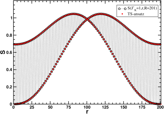
Figure 10: DMRG results for $S(J^{\prime}_{K}=1,r,{R}=201)$ for the spin-chain model with $J_{2}=J/2$ (MG model). The small circles represent the theoretical result obtained using the ansatz Eq. (6.2) with variationally determined $\psi^{sol}_{n}$ (F).

6.1.2 TS-ansatz for the Entanglement entropy for ${R}$ even, $J^{\prime}_{K}=0$

It is now straight forward to extend our results from the previous section to the case where ${R}$ is even and $J^{\prime}_{K}=0$. Our starting point is the expression Eq. (2.9) for the reduced density matrix. In order to calculate $\rho_{\Downarrow\Downarrow}$ and in particular $\rho_{\Uparrow\Downarrow}$ we need an ansatz for $\Psi_{TS}^{\Downarrow}$ with all couplings uniform and total length $R^{\prime}=R-1$ odd with $r^{\prime}=r-1$ denoting the spatial coordinate. This can straightforwardly be obtained from Eq. (6.2) by inverting the soliton spin to obtain:

$$|\Psi_{TS}^{\Downarrow}\rangle\simeq\sum_{n=0}^{\frac{{R}^{\prime}-1}{2}}\psi^{sol}_{n}|\overbrace{-\ \ldots\ -}^{n}\ \downarrow\ -\ \ldots\ -\rangle.$$ (6.16)

Using this ansatz we can now evaluate $\rho_{\Downarrow\Downarrow}$ as well as $\rho_{\Uparrow\Downarrow}$.

As above, we start by separating Eq. (6.16) into contributions from region $A$ ($1\ldots r^{\prime}$) and $B$ ($r^{\prime}+1\ldots{R}^{\prime}$) again initially assuming that $r^{\prime}$ is odd. We write:

$$|\Psi_{TS}^{\Downarrow}\rangle=\sum_{i,j=0}^{3}C_{i,j}|\psi_{i}^{\prime}\rangle|\phi_{j}^{\prime}\rangle,$$ (6.17)

with the $|\psi_{i}^{\prime}\rangle$ states in the Hilbert space for region $A$ and the $|\phi_{j}^{\prime}\rangle$ states in the Hilbert space for region $B$. In this case it is convenient to define $|\psi_{i}^{\prime}\rangle$:

$$|\psi_{1}^{\prime}\rangle = \sum_{n=0}^{\frac{r^{\prime}-1}{2}}\psi^{sol}_{n}|\overbrace{-\ \ldots\ -}^{n}\ \downarrow\ -\ \ldots\ -\rangle$$

$$|\psi_{2}^{\prime}\rangle = |\overbrace{-\ -\ -\ \ldots\ -\ -\ -\ }^{\frac{r^{\prime}-1}{2}}\ \downarrow\rangle$$

$$|\psi_{3}^{\prime}\rangle = |\overbrace{-\ -\ -\ \ldots\ -\ -\ -\ }^{\frac{r^{\prime}-1}{2}}\ \uparrow\rangle.$$ (6.18)

For $|\phi_{j}^{\prime}\rangle$ we write:

$$|\phi_{1}^{\prime}\rangle = |\overbrace{-\ -\ -\ \ldots\ -\ -\ -\ }^{\frac{{R}^{\prime}-r^{\prime}}{2}}\rangle$$

$$|\phi_{2}^{\prime}\rangle = \sum_{n=0}^{\frac{{R}^{\prime}-r^{\prime}}{2}-1}\psi^{sol}_{\frac{r^{\prime}+1}{2}+n}|\uparrow\ \overbrace{-\ \ldots\ -}^{n}\ \downarrow\ -\ \ldots\ -\rangle$$

$$|\phi_{3}^{\prime}\rangle = \sum_{n=0}^{\frac{{R}^{\prime}-r^{\prime}}{2}-1}\psi^{sol}_{\frac{r^{\prime}+1}{2}+n}|\downarrow\ \overbrace{-\ \ldots\ -}^{n}\ \downarrow\ -\ \ldots\ -\rangle.$$

With these definitions one finds that $\langle\psi_{i}|\psi_{j}\rangle=\langle\psi_{i}^{\prime}|\psi_{j}^{\prime}\rangle$ and $\langle\phi_{i}|\phi_{j}\rangle=\langle\phi_{i}^{\prime}|\phi_{j}^{\prime}\rangle$. Hence, for this choice of states, $\rho_{\Downarrow\Downarrow}$ is numerically identical to $\rho_{\Uparrow\Uparrow}$, Eq. (6.15). However, the actual states $|\phi_{j}^{\prime}\rangle$ are not identical to the $|\phi_{j}\rangle$ and $\langle\phi_{i}|\phi^{\prime}_{j}\rangle$ is not the identity matrix. This becomes important for the evaluation of $\rho_{\Uparrow\Downarrow}$ which can be expressed:

$$\rho_{\Uparrow\Downarrow}(i_{1},i_{2})=\sum_{j_{1},j_{2}=1}^{3}\tilde{C}_{i_{1},j_{1}}\tilde{C}_{i_{2},j_{2}}\langle\phi_{j_{1}}|\phi_{j_{2}}^{\prime}\rangle,$$ (6.20)

with the coefficient matrix $\tilde{C}$ given as before by Eq. (6.14). It is easily seen that $\langle\phi_{i}|\phi_{j}^{\prime}\rangle=0$ except for $\langle\phi_{1}|\phi_{1}^{\prime}\rangle=\langle\phi_{1}|\phi_{1}\rangle$, $\langle\phi_{2}|\phi_{1}^{\prime}\rangle=\langle\phi_{2}|\phi_{1}\rangle$ and $\langle\phi_{1}|\phi_{2}^{\prime}\rangle=\langle\phi_{1}|\phi_{2}\rangle$. $\rho_{\Uparrow\Downarrow}$ can then be evaluated along with $\rho_{\Downarrow\Uparrow}=\rho^{\dagger}_{\Uparrow\Downarrow}$ and the full density matrix, Eq. (2.9), describing $J^{\prime}_{K}=0$ and ${R}$ even constructed. Again, by essentially interchanging the role of $|\psi_{i}^{\prime}\rangle$ and $|\phi_{j}^{\prime}\rangle$, it is straightforward to obtain results for $r^{\prime}=r-1$ even as well.

With the matrices, $\rho_{\Uparrow\Uparrow}$, $\rho_{\Downarrow\Downarrow}$, $\rho_{\Uparrow\Downarrow}$$\rho_{\Downarrow\Uparrow}$ in hand, the full density matrix for $J^{\prime}_{K}=0$ and ${R}$ even can be constructed from Eq. (2.9) and the complete entanglement entropy calculated.

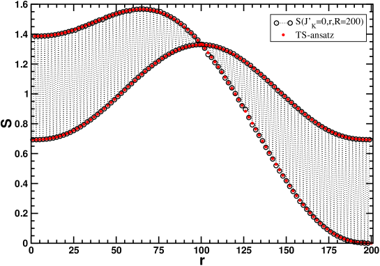
Figure 11: DMRG results for $S(J^{\prime}_{K}=0,r,{R}=200)$ for the spin-chain model with $J_{2}=J/2$ (MG model). The solid line represents the theoretical result obtained using the TS-ansatz Eq. (6.2) and Eq. (6.16) with variationally determined $\psi^{sol}_{n}$ (F).

As an example of how well the TS-ansatz, Eq. (6.2) and Eq. (6.16), work we show in Fig. 11 the results of a calculation of $S(J^{\prime}_{K}=0,r,{R}=200)$ using this approach compared with DMRG results for the same quantity with variationally determined $\psi^{sol}_{n}$ (F). Excellent agreement is observed. The small discrepancies between the DMRG results and the TS-ansatz visible at a few $r$ values are due to complications using spin-inversion in the DMRG calculations specific to this value of $J_{2}$.

We end this section by remarking that in principle the TS-ansatz could be used for any $J_{2}>J^{c}_{2}$ by simply redoing the variational calculation determining the $\psi^{sol}_{n}$.

6.2 The Orthonormal Thin Soliton (OTS) Ansatz

While relatively straight forward to use, the TS-ansatz does not yield expressions that are intuitively easy to grasp. It therefore seems desirable to develop a simplified picture of the underlying physics which we will now try to do. We shall do this by assuming that the TS states are orthonormal, thereby arriving at a simplified ansatz. Within this simplified ansatz the “single particle entanglement” and “impurity valence bond” contributions to the entanglement entropy, introduced in in sub-section 3, are derived explicitly employing this ansatz.

6.2.1 OTS-ansatz for the Entanglement entropy for ${R}$ odd, $J^{\prime}_{K}=1$

We begin by focusing on the case of ${R}$ odd and $J^{\prime}_{K}=1$ at the MG-point ($J_{2}=J/2$). Our starting point for the calculation of this quantity using the TS-ansatz was the expression $|\Psi^{\Uparrow}>=\sum_{i,j}C_{i,j}|\psi_{i}\rangle|\phi_{j}\rangle$. We now make the simplifying assumption that all the $|\psi_{i}\rangle$ and $|\phi_{j}\rangle$ are orthonormal. We shall refer to this as the orthonormal thin soliton ansatz (OTS-ansatz). This does not change the coefficients $C_{i,j}$: $C_{1,1}=1,C_{2,2}=-C_{3,3}=1/\sqrt{2}$ and $0$ otherwise. However, the reduced density matrix now significantly simplifies and assuming orthonormality we find for $r$ odd:

$$\rho^{\perp}_{\Uparrow\Uparrow}=\left(\begin{array}[]{ccc}\sum_{n=0}^{k-1}|\psi^{sol}_{n}|^{2}&0&0\cr 0&\frac{1}{2}\sum_{n=k}^{N_{d}}|\psi^{sol}_{n}|^{2}&0\cr 0&0&\frac{1}{2}\sum_{n=k}^{N_{d}}|\psi^{sol}_{n}|^{2}\cr\end{array}\right).$$ (6.21)

Here, $k=(r+1)/2$ and, as above, $N_{d}=({R}-1)/2$. If we by $p$ denote the probability that the soliton is to the left of the point $r$ we then see that this is simply:

$$\rho^{\perp}_{\Uparrow\Uparrow}=\left(\begin{array}[]{ccc}p&0&0\cr 0&\frac{1-p}{2}&0\cr 0&0&\frac{1-p}{2}\cr\end{array}\right),\ r\ \mathrm{odd}.$$ (6.22)

It immediately follows that for $r$ odd:

$$S(J^{\prime}_{K}=1,r,{R})=-p\ln(p)-(1-p)\ln(1-p)+(1-p)\ln(2).$$ (6.23)

If we now turn to $r$ even while still considering ${R}$ odd and $J^{\prime}_{K}=1$ we instead find:

$$\rho^{\perp}_{\Uparrow\Uparrow}=\left(\begin{array}[]{ccc}1-p&0&0\cr 0&\frac{p}{2}&0\cr 0&0&\frac{p}{2}\cr\end{array}\right),\ r\ \mathrm{even}.$$ (6.24)

This naturally follows from the fact that now $\rho^{\perp}_{1,1}$ describes a situation with the soliton to the right of the point $r$ while $\rho^{\perp}_{2,2}$ and $\rho^{\perp}_{3,3}$ have the soliton the left. We then see that in this case for $r$ even:

$$S(J^{\prime}_{K}=1,r,{R})=-p\ln(p)-(1-p)\ln(1-p)+p\ln(2).$$ (6.25)

We emphasize that Eq. (6.23) and (6.25) precisely equal the heuristic expression Eq. (3.5) based on the SPE and IVB.

We can now explicitly obtain expressions for the uniform and alternating part of the entanglement entropy, we find for ${R}$ odd:

$$S_{U}(J^{\prime}_{K}=1,r,{R}) = -p\ln(p)-(1-p)\ln(1-p)+\frac{1}{2}\ln(2)$$ (6.26)

$$S_{A}(J^{\prime}_{K}=1,r,{R}) = (\frac{1}{2}-p)\ln(2).$$ (6.27)

From this we can immediately extract $S_{imp}(J^{\prime}_{K}=1,r,{R})$ for ${R}$ odd since at the MG-point $S_{U}(J_{K}^{\prime}=1,r,{R})$ for ${R}$ even is simply $\ln(2)/2$ for any $r$. We then find:

$$S_{imp}(J^{\prime}_{K}=1,r,{R})=-p\ln(p)-(1-p)\ln(1-p),{R}\ \mathrm{odd}.$$ (6.28)

Since this is effectively the entanglement resulting from the presence of a single thin soliton in the ground-state we see that the $S_{imp}$ in this case is given uniquely by the SPE.

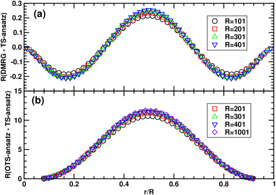
Figure 12: Comparison of results for $S_{imp}(J_{K}^{\prime}=1,r,{R})$ at the MG-point $J_{2}=J/2$ for a range of system sizes obtained using DMRG, TS-ansatz and the OTS-ansatz. (a) Difference between DMRG results and TS-ansatz results scaled by ${R}$. (b) Difference between OTS and TS-ansatz results scaled by ${R}$. For the TS-ansatz variationally determined $\psi^{sol}_{n}$ (F) have been used where as for the OTS-ansatz the analytical result for $p(r)$ Eq. (6.38) have been used.

It is of considerable interest to test how well the TS- and OTS-ansatz agree at the MG-point and to test how well either one of them agree with the DMRG results. In Fig. 12(a) we show results for the difference between $S_{imp}(J_{K}^{\prime}=1,r,{R})$ calculated with DMRG and the TS-ansatz scaled by ${R}$. Fig. 12(b) shows results for the difference between $S_{imp}(J_{K}^{\prime}=1,r,{R})$ calculated with the OTS-ansatz, Eq. (6.28), and with the TS- ansatz, again scaled by ${R}$. The data in Fig. 12 clearly show that in the thermodynamic limit all three approaches agree. This somewhat surprising result indicates that at the MG-point the non-orthogonality of the TS-states for the calculation of the entanglement entropy cannot play an important role.

6.2.2 OTS-ansatz for the Entanglement entropy for ${R}$ even, $J^{\prime}_{K}=0$

We now turn to the case where $J^{\prime}_{K}=0$ and ${R}$ is even. We then have to consider the full $6\times 6$ density matrix. If we initially take $r$ even we find (${R}$ even):

$$\rho^{\perp}=\left(\begin{array}[]{cccccc}\frac{p}{2}&0&0&-\frac{p}{2}&0&0\cr 0&\frac{1-p}{4}&0&0&0&0\cr 0&0&\frac{1-p}{4}&0&0&0\cr-\frac{p}{2}&0&0&\frac{p}{2}&0&0\cr 0&0&0&0&\frac{1-p}{4}&0\cr 0&0&0&0&0&\frac{1-p}{4}\cr\end{array}\right),\ r\ \mathrm{even}.$$ (6.29)

This follows from the observation that within the OTS ansatz and with the states $|\phi_{k}\rangle$ and $|\phi^{\prime}_{l}\rangle$ as defined in Eqs. (6.8) and (LABEL:eq:phipj), $\langle\phi_{k}|\phi^{\prime}_{l}\rangle=0$ unless $k=l=1$ in which case $\langle\phi_{1}|\phi^{\prime}_{1}\rangle=1$. By diagonalizing this matrix it follows that for $r$ even (${R}$ even):

$$S(J^{\prime}_{K}=0,r,{R})=-p\ln(p)-(1-p)\ln(1-p)+2(1-p)\ln(2).$$ (6.30)

In the same manner we write for $r$ odd (${R}$ even):

$$\rho^{\perp}=\left(\begin{array}[]{cccccc}\frac{1-p}{2}&0&0&0&0&0\cr 0&\frac{p}{4}&0&0&0&\frac{p}{4}\cr 0&0&\frac{p}{4}&0&\frac{p}{4}&0\cr 0&0&0&\frac{1-p}{2}&0&0\cr 0&0&\frac{p}{4}&0&\frac{p}{4}&0\cr 0&\frac{p}{4}&0&0&0&\frac{p}{4}\cr\end{array}\right),\ r\ \mathrm{odd}.$$ (6.31)

In a way analogous to Eq. (6.29), we find non-zero off-diagonal elements. From which it follows that for $r$ odd (${R}$ even):

$$S(J^{\prime}_{K}=0,r,{R})=-p\ln(p)-(1-p)\ln(1-p)+\ln(2).$$ (6.32)

Again we emphasize that Eq. (6.30) and (6.32) precisely equal the heuristic expression Eq. (3.7) based on the SPE and IVB.

As above, we can now explicitly obtain expressions for the uniform and alternating part of the entanglement entropy, we find for ${R}$ even:

$$S_{U}(J^{\prime}_{K}=0,r,{R}) = -p\ln(p)-(1-p)\ln(1-p)+(\frac{3}{2}-p)\ln(2)$$ (6.33)

$$S_{A}(J^{\prime}_{K}=0,r,{R}) = (\frac{1}{2}-p)\ln(2).$$ (6.34)

We note that the uniform part is simply $\mathrm{SPE}+(3/2-p)\ln(2)$. Again we can immediately extract $S_{imp}(J^{\prime}_{K}=0,r,{R})$ for ${R}$ even at the MG-point by using the above result for $S_{U}(J_{K}^{\prime}=1,r,{R})$, Eq. (6.26). We find:

$$S_{imp}(J^{\prime}_{K}=0,r,{R})=(1-p)\ln(2),{R}\ \mathrm{even}.$$ (6.35)

We note that this expression does not contain a contribution from the single part entanglement (SPE), but purely a term related to the impurity valence bond (IVB).

By numerically calculating the density matrix $\rho$ for large ${R}$ using the TS-ansatz, we have verified that the $\rho$ indeed does follow the above approximate forms, Eqs. (6.29) and (6.31), for both $r$ even and odd.

It is useful to have an analytical expression for $p$, the probability of finding the soliton in region A $(x\leq r)$. Simplifying our expression for the soliton wavefunction, Eq. (6.5), we write:

$$\psi^{sol}(x)\simeq\sqrt{\frac{2}{{R}}}\sin\left(\frac{\pi x}{{R}}\right).$$ (6.36)

With $p$ corresponding to the probability of finding the particle in region A ($x\leq r$) we can then write:

$$p=\int_{0}^{r}|\psi^{sol}(x)|^{2}dx.$$ (6.37)

From which we find:

$$p=\frac{r}{{R}}-\frac{1}{2\pi}\sin\left(2\pi r/{R}\right).$$ (6.38)

This expression agrees rather well with the probability extracted from the variationally determined soliton wave-function. See F. Since $p$ only depends on the single variable $r/{R}$ we see that also $S_{imp}(J_{K}^{\prime}=0,r,{R})$ and $S_{imp}(J_{K}^{\prime}=1,r,{R})$ as obtained from the OTS-ansatz are functions of the single variable $r/{R}$. When we refer to the OTS-ansatz we always assume that $p(r)$ has been determined using the above analytical form, Eq. (6.38).

If a similar analysis had been performed away from the MG-point, at a different $J_{2}>J_{2}^{c}$, the soliton wave function, Eq. (6.36) would likely change and thereby the above expression for $p$. However, it is noteworthy that the remaining expressions such as Eqs. (6.28) and (6.35) only depend on $J_{2}$ through $p$.

7 Numerical Results for the Fixed Point Entanglement

7.1 Fixed Point Entanglement at the MG-point, $J_{2}=J/2$

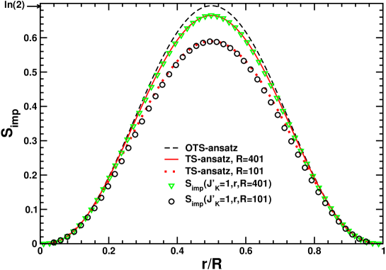
Figure 13: DMRG results for $S_{imp}(J^{\prime}_{K}=1,r,{R})$ for ${R}=101,401$ for the spin-chain model with $J_{2}=J/2$. The dashed line represents the OTS-ansatz result Eq. (6.28). For ${R}=101,401$ we also show the results for the TS-ansatz Eq. (6.2) as the solid and dotted lines.

At the MG-point ($J_{2}=J/2$) we can use the TS-ansatz, Eq. (6.2), directly to calculate $S_{imp}(J^{\prime}_{K}=1,r,{R})$ for ${R}$ odd. This is straight forward since $S(J^{\prime}_{K}=1,r,{R})$ for ${R}$ even is simply $\ln(2)$ for $r$ odd and zero otherwise. The result of such a calculation it the MG-point is shown in Fig. 13 (solid lines) for ${R}=101,401$ where we also show result for the same quantity calculated using the TS- and OTS-ansatz, Eqs. (6.2), with variationally determined $\psi^{sol}_{n}$, and (6.28) with $p(r)$ from Eq. (6.38). Note that, the TS-ansatz depends on ${R}$ where as the OTS-ansatz is independent of ${R}$. Excellent agreement is observed between the theoretical and numerical results. Both the DMRG results and TS-results rapidly approach the OTS result as implied by Fig. 12. Clearly this fixed point impurity entanglement entropy is non-zero at the MG-point and attains its maximum of $\ln(2)$ in the middle of the chain.

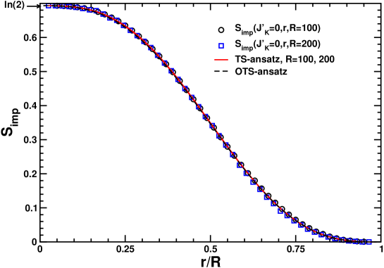
Figure 14: DMRG results for $S_{imp}(J^{\prime}_{K}=0,r,{R})$ for ${R}=100,200$ for the spin-chain model with $J_{2}=J/2$. The solid line represents the theoretical result Eq. (6.35).

Likewise, we can obtain $S_{imp}(J^{\prime}_{K}=0,r,{R})$ for ${R}$ even at the MG-point using the TS-ansatz with variationally determined $\psi^{sol}_{n}$. The results are indistinguishable from the OTS-ansatz, Eq. (6.35), with $p(r)$ from Eq. (6.38). Our results obtained at the MG-point are shown in Fig. 14 for system sizes ${R}=100,200$. Almost no variation with ${R}$ is observed and the numerical DMRG results display almost complete agreement with the TS- and OTS-ansatz. The TS- and OTS-ansatz yields results that are almost identical and the difference between the two is not visible in Fig. 14. The lack of finite-size effects is presumably related to the fact that $S_{imp}(J^{\prime}_{K}=0,r,{R})$ does not contain a contribution from the single particle entanglement entropy (SPE). $S_{imp}(J^{\prime}_{K}=0,r/{R})$ display a distinct cross-over between $\ln(2)$ and zero and clearly remains non-zero as ${R}\to\infty$.

7.2 Fixed Point Entanglement in the Dimerized Phase, $J_{2}^{c}\leq J_{2}<J/2$

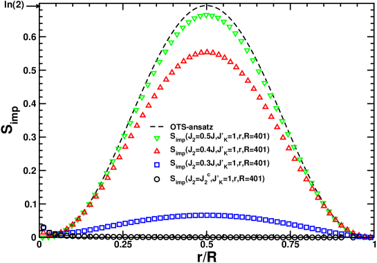
Figure 15: DMRG results for $S_{imp}(J^{\prime}_{K}=1,r,{R})$ for ${R}=401$ for the spin-chain model with $J_{2}=J_{2}^{c},0.3J,0.4J,0.5J$. The dashed line represents the OTS result Eq. (6.28), valid at the MG-point ($J_{2}=J/2$).

We now turn to a discussion of the variation of the fixed point entanglement entropies $S_{imp}(J_{K}^{\prime}=1,r/{R})$ and $S_{imp}(J^{\prime}_{K}=0,r/{R})$ with $J_{2}$ as we decrease $J_{2}$ towards the critical point $J_{2}^{c}$. In Fig. 15 we show DMRG results for $S_{imp}(J_{K}^{\prime}=1,r/{R})$ for $J_{2}=J^{c}_{2},0.3J,0.4J,0.5J$. In all cases with ${R}=401$. The dashed line represents the OTS-result, Eq. (6.28), with $p(r)$ from Eq. (6.38), valid at the MG-point. It is seen that $S_{imp}(J_{K}^{\prime}=1,r/{R})$ quickly diminishes as $J_{2}$ is decreased towards $J^{c}_{2}$. At $J_{2}^{c}$ we have argued in section 5 that $S_{imp}(J_{K}^{\prime}=1,r/{R})$ approaches zero in the thermodynamic limit. In fact, from the structure of the OTS-ansatz it is clear that this approximation must break down at the critical point since almost any form for the soliton wavefunction, $\psi^{sol}$, would imply a non-zero $p$ and thus a non-zero result in Eq. (6.28). We also note that at the critical point the soliton becomes massless.

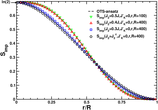
Figure 16: DMRG results for $S_{imp}(J^{\prime}_{K}=0,r,{R})$ for ${R}=400$ for the spin-chain model with $J_{2}=J_{2}^{c},0.3J,0.4J,0.5J$. The dashed line represents the OTS result Eq. (6.35).

We now focus on $S_{imp}(J_{K}^{\prime}=0,r/{R})$ for which we show DMRG results for $S_{imp}(J_{K}^{\prime}=1,r/{R})$ with $J_{2}=J^{c}_{2},0.3J,0.4J,0.5J$ in Fig. 16. The dashed line represents the OTS-result Eq. (6.35), with $p(r)$ from Eq. (6.38), valid at the MG-point. Although some variation of $S_{imp}(J_{K}^{\prime}=0,r/{R})$ with $J_{2}$ is seen, this variation is rather small and this fixed point impurity entanglement entropy clearly remains non-zero at the critical point, $J_{2}^{c}$. There are some finite size effects but at $J_{2}^{c}$ these affects are rather small. Perhaps surprisingly, the OTS result Eq. (6.35) is not dramatically different from the DMRG results even at the critical point $J_{2}^{c}$. We speculate that this is due to the fact that $S_{imp}(J_{K}^{\prime}=0,r/{R})$ does not contain a contribution from the single particle entanglement but can be described entirely in terms of the impurity valence bond picture. $S_{imp}(J_{K}^{\prime}=1,r/{R})$, on the contrary, is completely described by the single particle entanglement.

7.3 Fixed Point Entanglement in the Gapless Heisenberg Phase, $J_{2}<J_{2}^{c}$

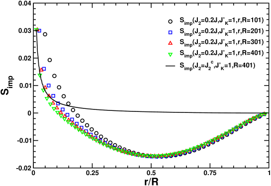
Figure 17: DMRG results for $S_{imp}(J_{2}=0.2J,J^{\prime}_{K}=1,r,{R})$ for ${R}=101,201,301,401$ for the spin-chain model with $J_{2}=0.2J$. The solid line is DMRG results for $S_{imp}(J_{2}=J_{2}^{c},J^{\prime}_{K}=1,r,{R}=401)$ calculated at the critical point, $J_{2}=J_{2}^{c}$.

Finally we turn to the gapless Heisenberg phase where $J_{2}<J_{2}^{c}$. Our results for $S_{imp}(J_{2}=0.2J,J_{K}^{\prime}=1,r/{R})$ are shown in Fig. 17 for a series of system sizes, ${R}=101,201,301$ and $401$ all calculated at $J_{K}^{\prime}=0.2J$. For comparison we have included results for $S_{imp}(J_{2}=J_{2}^{c},J_{K}^{\prime}=1,r/{R})$ at the critical point. It is seen that $S_{imp}(J_{2}=0.2J,J_{K}^{\prime}=1,r/{R})$ is rather small and negative for this value of $J_{2}$ with relatively little variation with the system size ${R}$. In comparison $S_{imp}(J_{2}=J_{2}^{c},J_{K}^{\prime}=1,r/{R})$ remains positive. A likely explanation for this is that the single particle entanglement, largely characterizing $S_{imp}(J^{\prime}_{K}=1,r/{R})$, is very sensitive to $J_{2}$ and no longer is a sensible quantity for $J_{2}<J_{2}^{c}$ due to the gapless nature of this phase.

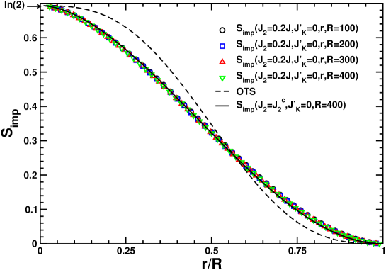
Figure 18: DMRG results for $S_{imp}(J_{2}=0.2J,J^{\prime}_{K}=0,r,{R})$ for ${R}=100,200,300,400$ for the spin-chain model with $J_{2}=0.2J$. The dashed line represents the OTS result Eq. (6.35). The solid line are DMRG results for $S_{imp}(J_{2}=J_{2}^{c},J^{\prime}_{K}=0,r,{R}=400)$ calculated at the critical point, $J_{2}=J_{2}^{c}$.

Results for $S_{imp}(J_{2}=0.2J,J^{\prime}_{K}=0,r,{R})$ for ${R}=100,200,300,400$ are shown in Fig. 18 for $J_{2}=0.2J$. We also show results for $S_{imp}(J^{\prime}_{K}=0,r,{R}=400)$ calculated at the critical point, $J_{2}=J_{2}^{c}$. In this case the results at $J_{2}=0.2J$ are very similar to the results at the critical point $J_{2}=J_{2}^{c}$ and it seems possible that the results coincide in the thermodynamic limit. We speculate that the fixed point entanglement found at the critical point is representative for all of the gapless Heisenberg phase $J_{2}<J_{2}^{c}$.

8 The alternating part, $S_{A}$

8.1 General discussion

Entanglement entropy in spin chains also has an interesting staggered part as we pointed out in [87]. For an open chain with no impurity, this was shown to decay away from the boundary with a power law $1/2$, the same power-law exhibited by the dimerization. The operator of dimension 1/2, representing the dimerization, is related by a chiral SU(2) transformation to the staggered spin density, $\vec{n}$, reviewed in A. It has no counterpart in a non-interacting fermion system. (Or, more correctly, the counterpart, while it exists, must always come together with the operator $\cos\phi_{c}$ from the charge sector as reviewed in A).) This alternating entropy for the open chain with no impurity decays with a different exponent than what occurs for an open chain of free fermions [87]. If we now include a weak coupling of an impurity spin to the end of the chain, we expect that the associated change in the alternating part of the entanglement entropy will continue to be different that of the free fermion Kondo model. This is in striking contrast to the uniform part which we have argued to be the same (at long length scales) for free fermion and spin chain Kondo models. In the rest of this section we discuss the behavior of the dimerization and examine the behavior of the alternating part of the entanglement entropy for both critical and dimerized spin chains.

8.2 The Alternating Part of the Energy Density, $E_{A}$

We start by deriving a field theory epxression for the alternating part of the energy density, $E_{A}$, that we shall find sheds some light on the alternating part of the entanglement entropy. The energy density for XXZ antiferromagnetic spin chains:

$$\left\langle h_{r}\right\rangle=\left\langle(S_{r}^{+}S_{r+1}^{-}+S_{r}^{-}S_{r+1}^{+})/2+\Delta S_{r}^{z}S_{r+1}^{z}\right\rangle$$ (8.1)

is uniform in periodic chains. On the other hand, an open end breaks translational invariance and there will be a slowly decaying alternating term or ”dimerization” in the energy density

$$\left\langle h_{r}\right\rangle=E_{U}(r)+(-1)^{r}E_{A}(r),$$ (8.2)

where $E_{A}(r)$ becomes nonzero near the boundary and decays slowly away from it. We can calculate $E_{A}(r)$ by Abelian bosonization modified by open boundary conditions [106]. In the critical region $\left|\Delta\right|\leq 1$, the low energy effective Hamiltonian is just a free massless relativistic boson.

The staggered part of $h_{r}\sim(-1)^{r+1}(\psi_{R}^{\dagger}\psi_{L}-\psi_{L}^{\dagger}\psi_{R})\sim(-1)^{r+1}\sin(\sqrt{4\pi K}\phi)$. Here we follow the notation of Ref. [107], but define the Luttinger parameter as $K=\pi/(2(\pi-\cos^{-1}\Delta))$ so that $K=1$ for an $XY$ spin chain and $K=1/2$ for the Heisenberg model. In a system with finite ${{R}}$ and open boundary conditions,

$$E_{A}(r,{{R}})\propto\left\langle\sin(\sqrt{4\pi K}\phi)\right\rangle\propto\frac{1}{[\frac{2{{R}}}{\pi}\sin(\frac{\pi r}{{{R}}})]^{K}}.$$ (8.3)

This is our basic result for $E_{A}$, from which it follows that $E_{A}(r,{R})=f(r/{R})/\sqrt{{R}}$ for the Heisenberg model but $E_{A}(r,{R})=f(r/{R})/{R}$ for an $XY$ spin chain, corresponding to free fermions.

At the Heisenberg point, $\Delta=1$, Eq. (8.3) will have some logarithmical corrections due to the presence of a marginally irrelevant coupling constant, $g$, in the low energy Hamiltonian, Eq. (1.16), that we now try to take into account. This interaction is reviewed in A. Ignoring boundaries, the staggered energy density $E_{A}\sim\sin(\sqrt{2\pi}\phi)$ has the anomalous dimension

$$\gamma(g)=1/2-3g/4.$$ (8.4)

With a boundary, the renormalization group equation for $E_{A}$ is the naive one, involving the anomalous dimension, $\gamma(g)$ in the usual way.

$$[\partial/\partial(\ln r)+\beta(g)\partial/\partial g+\gamma(g)]E_{A}(r,r/{R})=0.$$ (8.5)

(Here the partial derivative with respect to $r$ is taken with $r/{R}$ held fixed.)

This result may require some justification since, in general, the presence of a boundary can strongly affect the scaling behavior. It is crucial here that we are considering $E_{A}$ far from the boundary compared to the ultraviolet cut-off (i.e. $r\gg 1$). The boundary condition dictates that we should regard the right moving factor in the operator $e^{i\sqrt{2\pi}\phi(r)}$, which occurs here as a left moving operator at the reflected point $-r$:

$$e^{i\sqrt{2\pi}\phi(r)}=e^{i\sqrt{2\pi}(\phi_{L}(r)+\phi_{R}(r))}\to e^{i\sqrt{2\pi}(\phi_{L}(r)-\phi_{L}(-r))}.$$ (8.6)

To calculate the anomalous dimension of this bi-local operator we can consider the operator product expansion (OPE) with the marginal interaction (reviewed in A). This marginal interaction, $\cos\sqrt{8\pi}\phi$ also becomes bi-local in the presence of the boundary. The OPE of these two bilocal operators, $e^{i\sqrt{2\pi}(\phi_{L}(r)-\phi_{L}(-r))}$ and $e^{-i\sqrt{8\pi}(\phi_{L}(r)-\phi_{L}(-r))}$ is the produce of the OPE’s of the operators at $\pm r$ separately. Fortunately, this gives exactly the same result as without the boundary. Therefore we expect the naive RG equation to apply.

The general solution of Eq. (8.5) is

$$E_{A}(r,r/{R})=F[g(r),r/{R}]\exp\{-\int_{r_{0}}^{r}d(\ln r^{\prime})\gamma[g(r^{\prime})]\},$$ (8.7)

where $F$ is an arbitrary function of $g(r)$ and $r/{R}$.

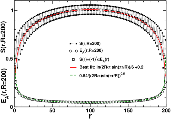
Figure 19: Entanglement entropy $S(r)$ (black squares) and alternating part of the energy density $E_{A}(r)$ (open circles) computed with DMRG at $J_{2}^{c}$ for $R=200$ sites. The dashed line is Eq. (8.3). The uniform part of $S(r)$, obtained by taking $S(r)+(-1)^{r}\alpha E_{A}(r)$ with $\alpha=1.001699$, is represented by open squares. The best fit, shown by a red curve, is indicated on the plot.

In the weak coupling limit, we may evaluate the scaling function $F(g(r),r/{R})$ at $g(r)=0$ and with the second order beta function, $\beta=-g^{2},$ we obtain: $E_{A}(r,r/{R})=F(r/{R})/[\sqrt{r}(\ln\left|r\right|)^{3/4}]$. One can push this a bit further following a similar calculation in Ref. [98, 108]. Provided with the beta function up to third order

$$\beta(g)=g^{2}-(1/2)g^{3},$$ (8.8)

the effective coupling solved from Eq. (8.8) is

$$\frac{1}{g(r)}-\frac{1}{g_{0}}=\{\ln(r/r_{0})+\frac{1}{2}\ln[\ln(r/r_{0})]\},$$ (8.9)

and expanding $F(g(r),r/{R})$ in powers of $g(r),$ we can improve the solution as

$$E_{A}(r,r/{R}) = \frac{F(r/{R})}{\sqrt{r}[\ln(r/a_{1})+\frac{1}{2}\ln\ln(r/a_{1})]}$$ (8.10)

$$\cdot\left\{1+\frac{a_{2}}{[\ln(r/a_{1})]^{2}}\right\},$$

where a term proportional to $1/[\ln(r/a_{1})]$ which could have occurred inside the curly brackets can always be adsorbed by redefining $a_{1}$. Note that since $r/{R}$ is being held fixed here, as we take $r\to\infty$, it follows that we can always replace $r$ by ${R}$ inside the logarithms in Eq. (8.10) by rescaling $a_{1}$ by ${R}/r$.

As reviewed in A, at the critical value of $J_{2}$, the marginal coupling constant vanishes and all logarithmic corrections vanish. Hence, we can check Eq. (8.3) directly using our DMRG results if we work at the critical point $J_{2}^{c}$. This is shown in Fig. 19 where results for $E_{A}(r,R=200)$ for a uniform ($J^{\prime}_{K}=1)$ system with $R=200$ are plotted along with Eq. (8.3). The agreement is quite good. In Ref. [87] it was argued that the alternating part of the entanglement entropy is given by $S_{A}=-\alpha E_{A}$. With $\alpha=1.001699$ we show $S(r,R)+(-1)^{r}\alpha E_{A}(r,R)$ in Fig. 19 and excellent agreement with this quantity and the uniform part of $S(r,R)$ is observed. Fitting this uniform part to Eq. (2.3) and using the fact that [107] $\ln g=-(1/4)\ln 2$ we estimate $s_{1}\simeq 0.746$.

8.3 Scaling of $S^{A}_{imp}$ at $J_{2}^{c}$

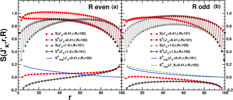
Figure 20: (a) DMRG results for the total entanglement entropy, $S(J^{\prime}_{K},r,R)$ for a 102 site spin chain at $J^{c}_{2}$, with a $J^{\prime}_{K}=0.41$ Kondo impurity ($\blacksquare$) along with $S(J^{\prime}_{K}=1,r-1,R-1)$ ($\square$). For both cases is the extracted alternating part shown along with the resulting $S^{A}_{imp}(J^{\prime}_{K}=0.41,r,R=102)$ for $R$ even. (b) DMRG results for the total entanglement entropy, $S(J^{\prime}_{K},r,R)$ for a 101 site spin chain at $J^{c}_{2}$, with a $J^{\prime}_{K}=0.41$ Kondo impurity ($\blacksquare$) along with $S(J^{\prime}_{K}=1,r-1,R-1)$ ($\square$). For both cases is the extracted alternating part shown along with the resulting $S^{A}_{imp}(J^{\prime}_{K}=0.41,r,R=101)$ for $R$ odd. For comparison we also show $S^{A}_{imp}(J^{\prime}_{K}=0.41,r,R=102)$ for $R$ even from panel (a) (dashed line).

Our fundamental definition of $S_{imp}$, Eq. (2.4), focused only on the uniform part of the entanglement entropy. It is also possible to define the alternating part of the impurity entanglement entropy following Eq. (2.4):

$$S^{A}_{imp}(J^{\prime}_{K},r,{{R}})\equiv S_{A}(J^{\prime}_{K},r,{{R}})-S_{A}(1,r-1,{{R}}-1).$$ (8.11)

As before, we have subtracted $S_{A}$ when the impurity is absent, in which case both $r$ and ${R}$ are reduced by one and the coupling at the end of this reduced chain, linking site $2$ to $3$ and $4$, has unit strength. Applying this definition to numerical data involves some subtleties. First of all $S^{A}$ is only defined up to an overall sign. Secondly, when calculating $S_{A}(1,r-1,{{R}}-1)$ we define this as $-S_{A}(1,r^{\prime},{{R}}^{\prime})$ with $R^{\prime}=R-1$ since the shift from $r$ to $r-1$ implies a sign change in the alternating part. For convenience we have therefore always exploited this degree of freedom to use a sign convention that makes the resulting $S^{A}_{imp}$ positive in all cases. In Fig. 20 we show data for the total entanglement entropy along with the extracted alternating parts and the resulting $S^{A}_{imp}$ for both $R=102$ even and $R=101$ odd. The initial data are the same as shown in Fig. 3 with $\xi_{K}=25.65$. As was the case for $S_{imp}$ we do not observe any special features in $S^{A}_{imp}(r)$ for fixed $R,J_{K}^{\prime}$ associated with the length scale $\xi_{K}$ and in all cases $S^{A}_{imp}$ decays monotonically with $r$.

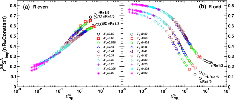
Figure 21: $\sqrt{r}S^{A}_{imp}$ for fixed $r/R$ and a range of couplings $J^{\prime}_{K}$ at $J_{2}^{c}$. (a) for $R$ even and (b) for $R$ odd. The values of $\xi_{K}$ used are obtained from the scaling of $S_{imp}$ and are listed in table 1. DMRG results with $m=256$ states.

We now turn to a discussion of a possible scaling form for $S^{A}_{imp}$. In Ref. [87] it was shown that for $J_{K}^{\prime}=1$ the alternating part of the entanglement entropy, $S^{A}$, is proportional to the alternating part in the energy, $E_{A}$ and it was shown that $E_{A}(r)=f(r/R)/\sqrt{(}r)$ for some scaling function $f$. See also the detailed derivation in subsection 8.2. A first guess for a scaling for $S_{imp}^{A}$ would then simply follow a generalization of the above formula to the case $J_{K}^{\prime}\neq 1$. Naively, this would imply that $\sqrt{(}r)S^{A}_{imp}$ should be a scaling function, $f(r/R,r/\xi_{K})$. Our results for $\sqrt{(}r)S^{A}_{imp}$ for fixed $r/{R}$ are shown in Fig. 21 for a range of $J^{\prime}_{K}$ and ${R}$. The values for $\xi_{K}$ used to attempt the scaling are the ones previously determined from the scaling of $S_{imp}$ for fixed $r/{R}$ at $J_{2}^{c}$, listed in table 1. Clearly the results for $\sqrt{r}S^{A}_{imp}$ follow the expected scaling form. We expect that the scaling would have been better had we allowed the $\xi_{K}$ to vary instead of using the data from table 1.

8.4 Alternating Part of the Fixed Point Entanglement Entropy

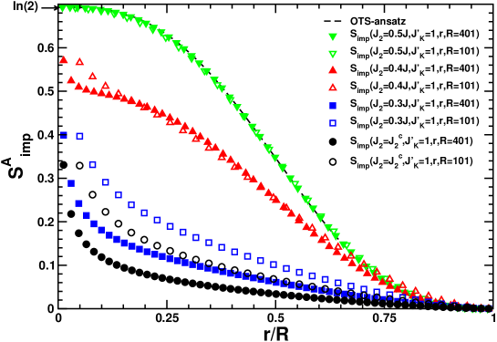
Figure 22: DMRG results for the alternating part of the fixed point entanglement, $S^{A}_{imp}(J_{2},J^{\prime}_{K}=1,r/R)$, shown for a range of values of $J_{2}=J_{2}^{c},0.3J,0.4J,0.5J$, in each case for 2 different values of $R=101,401$. The dashed line indicates the result for the OTS-ansatz, Eq. (8.12).

Following our definition of the alternating part of the impurity entanglement entropy, $S^{A}_{imp}$, given in Eq. (8.11), we can also analyze the alternating part of the fixed point entropy by studying $S^{A}_{imp}(J^{\prime}_{K}=0)$ and $S^{A}_{imp}(J^{\prime}_{K}=1)$. If we first focus on $S^{A}_{imp}(J^{\prime}_{K}=0)$ it is clearly zero when $R$ is odd as was the case for $S_{imp}(J^{\prime}_{K}=0)$. For $R$ even, we see from Eq. (6.34) and Eq. (6.27) that at the MG-point ($J_{2}=J/2$) the OTS-ansatz predicts that also in this case is $S^{A}_{imp}(J^{\prime}_{K}=0)$ zero. Numerical DMRG results confirms this and shows that also for $J_{2}<J/2$ is $S^{A}_{imp}(J^{\prime}_{K}=0)$ negligible. We have verified that this also holds at the critical point $J_{2}=J_{2}^{c}$ as well as in the gapless Heisenberg phase at $J_{2}=0.2J$.

The interesting fixed point entropy is then $S^{A}_{imp}(J^{\prime}_{K}=1)$. As for $S_{imp}(J^{\prime}_{K}=1)$, we see that the difference between $R$ even and $R$ odd amounts to a change of sign of the resulting fixed point entanglement entropy. We therefore only consider $R$ odd. At the MG-point we expect the OTS-ansatz to yield very precise results. If we combine Eq. (6.27) with the fact that for $R$ even $S^{A}(J^{\prime}_{K}=1)=\ln(2)/2$ for any $r$, we find the OTS result:

$$S^{A}_{imp}(J^{\prime}_{K}=1)=(1-p)\ln(2),\ R\ {\rm odd}.$$ (8.12)

Where $p$ is given in Eq. (6.38). As we mentioned in the previous section there is a slight subtlety here since, in order to calculate $S^{A}_{imp}(J^{\prime}K=1)$ for $R$ odd, we need $S_{A}(1,r-1,{{R}}-1)$ for $R-1$ even. Due to the shift, $r\to r-1$, we have defined this as $-\ln(2)/2$ as opposed to the $\ln(2)/2$ we just quoted. This sign convention renders the resulting fixed point entanglement entropy positive for all $r/R$. Choosing the other possible sign convention would have resulted in a trivial shift in the fixed point entanglement entropy of $\ln(2)$, yielding $-p\ln(2)$.

Our numerical DMRG results for $S^{A}_{imp}(J^{\prime}_{K}=1)$ for $R$ odd as a function of $r/R$ are shown in Fig. 22 for a range of second nearest neighbor couplings $J_{2}=J_{2}^{c},0.3J,0.4J,0.5J$ throughout the dimerized phase $J_{2}^{c}\leq J_{2}\leq J/2$. In each case we show results for two system sizes $R=101$ and $401$. At the MG-point we see that finite size effects are minimal and the results for $R=101$ and $401$ agree very well. In both cases the agreement with the result from the OTS-ansatz, Eq. (8.12), shown as the dashed line, is almost perfect. As $J_{2}$ is decreased from the value of $J/2$ pronounced finite-size effects develop and the fixed point entanglement entropy clearly tends toward zero with increasing $R$. This is also true at the critical point, $J_{2}=J_{2}^{c}$. For clarity we have not shown results for $J_{2}=0.2J$ in the gapless phase where $S^{A}_{imp}(J^{\prime}_{K}=1,r/R)$ for both $R=101$ and $401$ is smaller than at the critical point.

9 Conclusions 

The presence of impurities will clearly affect the entanglement and we have here defined the impurity contribution to the entanglement entropy, $S_{imp}$. Using the equivalence of the electronic Kondo model and the $J_{1}-J_{2}$ spin chain model in the regime $J_{2}<J_{2}^{c}$ we have shown numerical evidence that $S_{imp}$ follows a scaling form $S_{imp}(r/\xi_{K},r/R)$ demonstrating the presence of the length scale $\xi_{K}$ associated with screening of the impurity. We have provided rather strong arguments in favor of this scaling and analytical results based on a Fermi liquid approach valid for $r\gg\xi_{K}$. The D-dimensional Kondo model has been shown to yield the same entanglement as the 1-D Kondo model which in turn is equivalent to the entanglement in the $J_{1}-J_{2}$ spin chain. The single-site entanglement obtained by only considering the entanglement of the impurity spin has been shown to display weak scaling violations. For $J_{2}>J_{2}^{c}$ in the dimerized phase we have shown that almost exact calculations are possible using the variational TS-ansatz. Simplifying the TS-ansatz we have shown that the contributions arising from impurity valence bonds (IVB) and single particle entanglement (SPE) naturally arise at the MG-point. Finally, we have argued that at finite temperatures the entanglement entropy for a sub-system $A$ of size $r$, $S(T)$, will approach the thermal entropy, $S_{th}(T)$, for $T\gg v/r$. In light of the generality of our model we expect our results to be quite widely applicable. The study of quantum impurity entanglement as it occurs in more complex models with many body ground-states displaying non-trivial order would clearly be of considerable interest.

Appendix A Review of field theory results on the Kondo effect and spin chains

The usual Kondo model describes electrons moving in 3 dimensions with a short range exchange interaction with a single S=1/2 impurity spin. No other electron-electron interactions are taken into account. Although similar conclusions can be arrived at more generally, the simplest case is where a free electron quadratic dispersion relation is assumed, and the Kondo interaction is taken to be a $\delta$-function, implying spherical symmetry. The Hamiltonian is given in Eq. (1.3).

Kondo model calculations are traditionally carried out by reducing the 3$D$ fermionic model of Eq. (1.3) to an equivalent 1$D$ fermionic model. This can be done by expanding $\psi(\vec{r})$:

$$\psi(\vec{r})=(1/r)\sum_{l,m}Y_{l,m}(\hat{r})\psi_{l,m}(r),$$ (1.1)

where the $Y_{l,m}(\hat{r})$ are the usual spherical harmonics, depending only on the direction of $\vec{r}$ and the $\psi_{l,m}(r)$ are 1$D$ quantum fields. The spherically symmetric $H$ of Eq. (1.3) reduces to a sum of commuting terms: $H=\sum_{l,m}H_{l,m}$. Due to the $\delta$-function interaction, all harmonics are non-interacting except for the $s$-wave. The higher harmonics contain only the centrifugal potential energy $V_{l}(r)=l(l+1)/2r^{2}$. A low energy form of the $l=0$ Hamiltonian is obtained by linearizing the dispersion relation around the Fermi surface, $\epsilon(k)=k^{2}/2m-\epsilon_{F}$, yielding a 1$D$ Dirac fermion theory on the half-line, $r>0$, coupled to the impurity spin at $r=0$. We introduce left and right movers by:

$$\psi_{l=0}(r)\approx e^{ik_{F}r}\psi_{R}(r)+e^{-ik_{F}r}\psi_{L}(r),$$ (1.2)

where $\psi_{L/R}(r)$ vary slowly and $k_{F}$ is the Fermi momentum.

$$H_{1D} \approx (iv/2\pi)\int_{0}^{R}dr[\psi_{L}^{\dagger}(d/dr)\psi_{L}-\psi_{R}^{\dagger}(d/dr)\psi_{R}]$$ (1.3)

$$+v\lambda_{K}\psi_{L}^{\dagger}(0)(\vec{\sigma}/2)\psi_{L}(0)\cdot\vec{S}.$$

Note that we have adopted an unconventional normalization for these 1D fermion fields:

$$\{\psi_{L/R}^{\dagger}(r),\psi_{L/R}(r^{\prime})\}=2\pi\delta(r-r^{\prime}).$$ (1.4)

Here $\lambda_{K}\propto J_{K}$ and the left and right movers obey a boundary condition: $\psi_{L}(0)=\psi_{R}(0)$ [77, 78, 79]. Up to some trivial geometric factors of $r$, all the physics of Eq. (1.3) can then be obtained from this 1$D$ fermion model. If the 3D system is originally defined inside a sphere of radius ${R}$, then the 1D system exists on a line of length ${R}$.

It is now very convenient to bosonize this 1D model. This allows for the introduction of separate bosonic fields representing the spin and charge degrees of freedom of the conduction electrons. The non-interacting free electron Hamiltonian can be written as a sum of decoupled spin and charge terms:

$$H_{0}=H_{s0}+H_{c0}.$$ (1.5)

The spin part can be written in terms of the spin current operators:

$$\vec{J}_{L/R}\equiv\psi^{\dagger}_{L/R}{\vec{\sigma}\over 2}\psi_{L/R},$$ (1.6)

as:

$$H_{s0}=(v/2\pi)\int_{0}^{{R}}dr(1/3)[\vec{J}_{L}\cdot\vec{J}_{L}+\vec{J}_{R}\cdot\vec{J}_{R}].$$ (1.7)

The free boundary condition on the fermion fields at $r=0$ implies a boundary condition in the continuum limit: $\psi_{L}(0)=-\psi_{R}(0)$ which in turn implies $\vec{J}_{L}(0)=\vec{J}_{R}(0)$. Since the Kondo interaction only involves $\vec{J}_{L}$ it can be written entirely in terms of the spin boson field.

$$H_{K}=v\lambda_{K}\vec{J}_{L}(0)\cdot\vec{S}.$$ (1.8)

(Actually, there are irrelevant operators which couple spin and charge sectors together, but these can be ignored in the low energy effective theory.)

It is actually possible to continue to the negative $r$ axis, defining:

$$\psi_{L}(-r)\equiv-\psi_{R}(r),\ \ (0<r<{R}).$$ (1.9)

This in turn implies that $\vec{J}_{R}(r)=\vec{J}_{L}(-r)$. The free spin Hamiltonian then becomes:

$$H_{s0}=(v/6\pi)\int_{-{R}}^{{R}}dr\vec{J}_{L}\cdot\vec{J}_{L}.$$ (1.10)

Imposing convenient boundary conditions on left and right fields at $r={R}$, we obtain the periodic boundary conditions in the left-moving formulation: $\vec{J}_{L}(-{R})=\vec{J}_{L}({R})$.

Now consider the $J_{1}$-$J_{2}$ spin chain model of Eq. (1.4). The connection between spin chains and the Kondo model was pointed out in [107, 109], using field theory arguments and in [100] the Hamiltonian of Eq. (1.4) with $J_{2}=0$ was, among others, solved exactly by Bethe ansatz noting connections with Kondo physics. The low energy theory can again be described by bosonization. One approach is to bosonize the weakly coupled Hubbard model at half-filling and then to extrapolate to strong coupling. We again obtain spin and charge bosons. The Hubbard interaction gives a gap to the charge boson field, which can thus be eliminated from the low energy theory. The spin operators at site $j$ can be represented:

$$\vec{S}_{j}\approx[\vec{J}_{L}+\vec{J}_{R}]+(-1)^{j}\hbox{constant}\cos\phi_{c}\cdot\vec{n}.$$ (1.11)

Here $\phi_{c}$ is the charge boson and $\vec{n}$ is the antiferromagnetic order parameter and can be written entirely in terms of the spin boson field. The Hubbard interaction makes $<\cos\phi_{c}>\neq 0$ so we may replace this factor by a constant:

$$\vec{S}_{j}\approx[\vec{J}_{L}+\vec{J}_{R}]+(-1)^{j}\hbox{constant}\cdot\vec{n}.$$ (1.12)

The low energy Hamiltonian is simply the spin part of the non-interacting electron Hamiltonian, $H_{s0}$, up to irrelevant operators. In particular, the spin current operators have the same Green’s functions as in the non-interacting model. The field $\vec{n}$ can also be expressed in terms of the non-interacting spin bosons. It is represented in terms of exponentials of bosons (in the usual abelian bosonization scheme).

Now suppose that the chain has a free end at $r=0$. The boundary conditions on the fermion fields can be translated into boundary conditions on the spin boson field. These can be seen to imply:

$$\vec{n}(0)\propto\vec{J}_{L}(0)=\vec{J}_{R}(0).$$ (1.13)

Now suppose that we weakly couple one additional spin to the spin chain, with a coupling constant $J_{k}^{\prime}\ll 1$. We may write the low energy effective Hamiltonian using bosonization. If the extra spin couples at the end of the chain then the resulting interaction term is particularly simple:

$$H_{K}\propto\vec{J}_{L}(0)\cdot\vec{S}.$$ (1.14)

The coupling constant here is proportional to $J_{K}^{\prime}$ but the constant of proportionality is non-trivial involving the proportionality constant in Eq. (1.13). It can be extracted by studying the end-to-end spin correlation function in the chain without the weakly coupled spin [55], yielding:

$$J_{K}^{\prime}\approx 1.3807\lambda_{K}.$$ (1.15)

Thus the same low energy effective Hamiltonian is obtained for the spin chain with a weakly coupled spin at the end as for the usual free fermion Kondo model.

Two caveats should be made here. First of all, if the weakly coupled spin couples to a point far from the end of the spin chain then a much different low energy effective Hamiltonian occurs. Secondly, even when the weakly coupled spin is at the end, there are subtle differences from the usual Kondo model due to differences in the irrelevant operators. In the free fermion model all irrelevant operators have dimensions of at least 3 and are strictly irrelevant. However, the spin chain model has a notorious marginally irrelevant operator in its low energy effective Hamiltonian.

$$\delta H=-(gv/2\pi)\vec{J}_{L}\cdot\vec{J}_{R}.$$ (1.16)

This leads to logarithmic corrections to essentially all low energy properties which are difficult to calculate in detail and cause problems with fitting numerical data. Fortunately, there is a way of avoiding this difficulty. As we vary $J_{2}$, this marginal coupling constant, $g$ also varies. For small $J_{2}$, $g>0$, and is marginally irrelevant. A critical point occurs at $J_{2}=J_{c}\approx.2412$. For larger $J_{2}$ the system goes into a gapped spontaneously dimerized phase. Right at the critical point $g=0$ and all logarithmic corrections vanish. Much better agreement between numerical simulations and field theory predictions can be obtained at this point. All remaining irrelevant operators are strictly irrelevant, leading only to corrections which vanish with power-laws of the energy (or inverse length) scale, not logarithms. In a separate paper[55], we study the $J_{2}=0$ Kondo spin chain model in more detail. Here we will focus on the $J_{2}=J_{c}$ case. Note that this is actually much closer to the free fermion version of the Kondo model. We note that Eq. (1.15) was obtained at $J_{2}=J_{c}$.

At low energies and long length scales, the effective Kondo coupling becomes large, and the effective Hamiltonian flows to the strong coupling fixed point. In the electron version of the Kondo model we may think of this fixed point as one where the impurity spin is “screened”, i.e. it forms a singlet with a conduction electron. The remaining electrons behave, at low energies and long length scales, as if they were non-interacting, except that they obey a modified boundary condition reflecting the fact that they cannot break up the singlet by occupying the same orbital as the screening electron. This modified boundary condition corresponds to a $\pi/2$ phase shift. Correspondingly in the spin chain Kondo model, the impurity spin gets “adsorbed into the chain” and no longer behaves like a paramagnetic spin at low energies and long distances. The leading corrections to this low energy long distance picture are described by lowest order perturbation theory in the leading irrelevant operator at the strong coupling fixed point. This is an interaction between the remaining conduction electrons, near the screened impurity. (It doesn’t involve the impurity itself since it is screened and doesn’t appear in the low energy effective Hamiltonian.) This leading irrelevant operator is $\vec{J}_{L}(0)\cdot\vec{J}_{L}(0)$[78, 79]. From (1.10), we see that this is proportional to the spin part of the free electron energy density. It is the entire energy density in the low energy effective Hamiltonian for the spin chain. The energy density has dimensions of (energy)/(length) so the corresponding coupling constant in the effective Hamiltonian must have dimensions of length. On general scaling grounds we expect it to be proportional to $\xi_{K}$. The precise constant of proportionality simple corresponds to giving a precise definition of what we mean by $\xi_{K}$. We adopt the convention:

$$H_{int}=-(\pi\xi_{K}){\cal H}_{s,L}(0).$$ (1.17)

Here the subscripts $s$ and $L$ are a reminder that this is the spin only part of the energy density for left movers. For the purpose of doing first order perturbation theory in $H_{int}$ for quantities like the susceptibility, specific heat or ground state energy, which are translationally invariant in $0^{th}$ order, we may replace [77] $H_{int}$ by:

$$H_{int}\to-[\pi\xi_{K}/(2L)]\int_{-R}^{R}{\cal H}_{s,L}(x).$$ (1.18)

This is equivalent to a length dependent reduction of the velocity:

$$v\to v[1-\pi\xi_{K}/(2R)].$$ (1.19)

This then implies that the susceptibility, which is $R/(2\pi v)$ in the absence of the Kondo impurity becomes:

$$\chi\to R/\{(2\pi v)[1-\pi\xi_{K}/(2R)]\} \approx R/(2\pi v)+\xi_{K}/(4v)$$ (1.20)

$$= R/(2\pi v)+1/(4T_{K}).$$

Thus the zero temperature impurity susceptibility is $1/(4T_{K})$. It is this form of the impurity susceptibility, simply related to the high temperature, free spin behavior, $1/(4T)$, which motivates the definition of $\xi_{K}$ (and hence $T_{K}=v_{F}/\xi_{K}$) implied by (1.17). We note that this interaction $H_{int}$ is present even in the absence of an impurity, for free fermions but then the coupling constant is of order a lattice constant. Similarly it is also present for the spin chain with no impurity (i.e. $J_{K}^{\prime}=1$) with a coupling constant of order a lattice constant. The effect of a weak Kondo coupling is to make this coupling constant large. We emphasize that this precise choice of definition of $T_{K}$ has no physical consequences. The power of Fermi liquid theory is to predict not only the form of low energy quantities but also ratios of various low energy quantities such as impurity susceptibility, impurity specific heat, resistivity, etc., corresponding to various generalized Wilson ratios. In the limit $\xi_{K}\ll r$, we can also calculate $S_{imp}$ using the FLT interaction of Eq. 1.17 in the lowest order perturbation theory.

Appendix B 3D to 1D reduction and entanglement entropy

In this appendix we prove that the impurity entanglement entropy is the same for the $D$ and one-dimensional Kondo model and consequently also for the spin chain model. We also present a new derivation of the free fermion entanglement entropy in D-dimensions.

With a spherically symmetric dispersion relation and Kondo interaction, as in Eq. (1.3), the Hamiltonian is a sum of terms acting on subspaces of different $l$, $m$ quantum numbers for single electrons. That is, the kinetic energy term, for each electron separates into such a sum and so does the Kondo interaction. If the Kondo interaction is a $\delta$-function then only the s-wave term is non-zero. If it is longer range there are small larger $l$ terms. However, according to the usually RG picture of the multi-channel Kondo model the largest term grows under renormalization and the others shrink, so that in the low energy effective Hamiltonian we can ignore the higher harmonics.

This form of $H$ implies that the ground state wave-function is a product of factors, one from each channel. This follows because the single-particle wave-functions all have definite $l$, $m$ quantum numbers. We may define electron creation operators $c^{\dagger}_{l,m,r}$ which create an electron at distance $r$ from the origin in the $l$, $m$ channel, and write the ground state as a product over $l$ and $m$ of factors for each $l$, $m$. Ignoring the Kondo interaction (as we can basically do for $l>0$) each factor just corresponds to the product of creation operators corresponding to a filled Fermi sea. (Each channel is filled up to the Fermi energy.) Including the Kondo interaction this factorization is still valid but the wave-function for channels with a Kondo interaction are non-trivial. So, of course, the pure density matrix $|\psi><\psi|$ is also a product of factors for each $l$, $m$.

Now consider tracing over the region outside a sphere of radius $r$. It is important here that we choose a sphere, not some other shape, so as to preserve the rotational symmetry. This should leave a reduced density matrix which is also a product over $l$ and $m$. This may be especially clear if we introduce an ultra-violet cut-off by only allowing the particles to sit on the surfaces of spheres at various distances from the origin. The reduced density matrix is obtained by tracing over all the spherical surfaces further from the origin than $r$. So we can write:

$$\rho(r)=\prod\rho_{l,m}(r).$$ (2.1)

Here each reduced density matrix, $\rho_{l,m}$ acts on a different sector of the Hilbert space. So we can write:

$$\ln\rho(r)=\sum_{l,m}\ln\rho_{l,m}(r).$$ (2.2)

Actually, this notation implies that each term is a product of a non-trivial operator in one channel and the identity operator in all the others. When we calculate tr$\rho\ln\rho$, we get a sum of terms like tr$\rho\ln\rho_{l,m}$. Because we can write a complete set of states as a set of products in each channel, the trace of an operator written in product form reduces to a product of traces. So:

$$\Tr\rho\ln\rho_{l,m}=[\prod_{(l^{\prime},m^{\prime})\neq(l,m)}\Tr\rho_{l^{\prime},m^{\prime}}]\Tr(\rho_{l,m}\ln\rho_{l,m}).$$ (2.3)

Since tr$\rho_{l^{\prime},m^{\prime}}=1$, we get:

$$\Tr[\rho\ln\rho]=\sum_{l,m}\Tr[\rho_{l,m}\ln\rho_{l,m}].$$ (2.4)

Now if we compare the zero Kondo coupling to finite Kondo coupling case, only the s-wave channel changes. (More correctly, for a finite range Kondo interaction there is also some change in the higher $l$ channels. However, this is presumably just a short distance effect and drops off much more quickly than the s-wave part. i.e. like $a/r$ where $r$ is a cut off scale, instead of $\xi_{K}/r$ for the s-wave.) So the impurity entanglement entropy for the 3D system is the same as for 1D. Exploiting the equivalence of the 1D Kondo model and the spin chain model the entanglement entropy is the same also for this model.

We remark that the well-known $r^{2}\ln r$ form of the entanglement entropy [110, 111, 112] for free fermions (at $R\to\infty$) can apparently be recovered from the decomposition into angular momentum channels. Note that the Hamiltonian for all $l>0$ contains a centrifugal potential:

$$H_{l,m}=-{1\over 2}{d^{2}\over dr^{2}}+{l(l+1)\over 4r^{2}}.$$ (2.5)

This centrifugal potential will not be too important when the size, $r$, of region $A$ is sufficiently large and $l$ is not too large. Thus we expect to recover essentially the usual 1D result $S=(1/6)\ln r$ for these values of $l$ and $m$. However, for large enough $l$, we expect the entanglement entropy to be reduced, and eventually to vanish at large $l$ for any fixed $r$. This can be seen from the fact that the density of electrons in region $A$ with angular momentum $l$ vanishes at large $l$. If the region $A$ is essentially empty there can’t be any entanglement. We may estimate the order of magnitude of $l$ at which the sphere of size $r$ becomes empty by simply comparing the centrifugal potential to the Fermi energy,

$$E_{F}\approx{l_{max}(l_{max}+1)\over 4r^{2}}.$$ (2.6)

This gives

$$l_{max}\approx 2r\sqrt{E_{F}}.$$ (2.7)

Thus we estimate the free fermion entanglement entropy in 3D as:

$$S(r)\approx(1/6)\ln r\sum_{l=0}^{l_{max}}(2l+1)\approx{E_{F}r^{2}\over 3}\ln r.$$ (2.8)

(The prefactor of $E_{F}\propto n^{-2/3}$ where $n$ is the electron density is only expected to be correct in order of magnitude. ) This argument generalizes to any dimension $D$, giving:

$$S\propto r^{D-1}\ln r.$$ (2.9)

Appendix C Separating Staggered and Uniform Parts 

In this appendix we derive the 7-point formula used for extracting the uniform and alternating parts of the entanglement entropy from the numerical data.

We focus on functions, $f$, defined on a set of discrete lattice sites $i$, with a uniform part, $u$, in addition to a staggered part, $s$:

$$f(i)=u(i)+(-1)^{i}s(i).$$ (3.1)

We assume that both $s$ and $u$ are slowly varying. Often $s$ and $u$ are extracted by using the simplest possible 2-point approximation

$$u(i) = \frac{f(i)+f(i+1)}{2}$$

$$s(i) = (-1)^{i}\frac{f(i)-f(i+1)}{2},$$ (3.2)

by effectively assuming that $u(i)\simeq u(i+1)$ and $s(i)\simeq s(i+1)$. This somewhat crude approximation has many drawbacks and is insufficient for the present study. We therefore focus on higher order n-point approximations by approximating $u$ and $s$ locally by polynomials. If one is interested in developing an n-point formula that is symmetric around the point of interest it is not possible to use the same degree of polynomial for both $u$ and $s$. For the present study the most frequently occurring case is $u$ varying more rapidly than $s$. We have then found it sufficient to develop a 7-point approximation by assuming that $u(i)\simeq ai^{3}+bi^{2}+ci+d$ and $s(i)=ei^{2}+fi+g$, arriving at the equations:

$$f(i-3) \simeq -27a+9b-3c+d-(9e-3f+g)$$

$$f(i-2) \simeq -8a+4b-2c+d+(4e-2f+g)$$

$$f(i-1) \simeq -a+b-c+d-(e-f+g)$$

$$f(i) \simeq d+g$$

$$f(i+1) \simeq a+b+c+d-(e+f+g)$$

$$f(i+2) \simeq 8a+4b+2c+d+(4e+2f+g)$$

$$f(i+3) \simeq 27a+9b+3c+d-(9e+3f+g)$$

Solving these equations for $d,g$ we immediately get:

$$u(i) = -\frac{15}{496}f(i-3)-\frac{1}{248}f(i-2)+\frac{71}{248}f(i-1)$$

$$+ \frac{1}{2}f(i)+\frac{137}{496}f(i+1)+\frac{1}{248}f(i+2)-\frac{1}{31}f(i+3)$$

$$s(i) = (-1)^{i}\big{[}\frac{15}{496}f(i-3)+\frac{1}{248}f(i-2)-\frac{71}{248}f(i-1)$$ (3.4)

$$+ \frac{1}{2}f(i)-\frac{137}{496}f(i+1)-\frac{1}{248}f(i+2)+\frac{1}{31}f(i+3)\big{]}$$

$$= (-1)^{i}(f(i)-u(i))$$

Appendix D Detailed Proof of limited $SU(2)$ invariance of $S$

In this appendix we show that the von Neumann entropy for a system in doublet state (${R}$ odd) is $SU(2)$ invariant. For ${R}$ even the ground-state is a non-degenerate singlet an $S$ is manifestly $SU(2)$ invariant.

Consider the case of ${R}$ odd, where the ground states form a spin doublet. The most general linear combination of the doublet of ground states can be written as a unitary transformation of the spin-up ground state:

$$|\psi>=U|\uparrow>.$$ (4.1)

Here we can choose

$$U=\exp[i(a_{x}S^{x}_{T}+a_{y}S^{y}_{T})]$$ (4.2)

so that

$$U|\uparrow> = [\cos|\vec{a}/2|\mathcal{I}+2\hat{a}\cdot\vec{S}_{T}\sin|\vec{a}/2|]|\uparrow>$$ (4.3)

$$= \cos|\vec{a}/2||\uparrow>+{\frac{(a_{x}-ia_{y})}{|\vec{a}|}}\sin|\vec{a}/2||\downarrow>,$$

with $\mathcal{I}$ the identity matrix and

$$\vec{S}_{T}\equiv\sum_{j=1}^{{R}}\vec{S}_{j},$$ (4.4)

and we have used the fact that the states $|\uparrow>$, $|\downarrow>$ transform like an S=1/2 doublet under SU(2) to treat the Taylor expansion of the exponential. Now we observe that:

$$U=U_{A}\otimes U_{B},$$ (4.5)

where

$$U_{A}=\exp[i\vec{a}\cdot\sum_{j=1}^{r}\vec{S}_{j}],\ \ U_{B}=\exp[i\vec{a}\cdot\sum_{j=r+1}^{{R}}\vec{S}_{j}].$$ (4.6)

Thus:

$$|\psi>=U_{A}\otimes U_{B}|\uparrow>.$$ (4.7)

The pure density matrix can then be written:

$$\rho=U_{A}\otimes U_{B}|\uparrow><\uparrow|U_{B}^{\dagger}\otimes U_{A}^{\dagger}.$$ (4.8)

It follows that the reduced density matrix is:

$$\rho_{A}^{U}=U_{A}\rho_{A}U^{\dagger},$$ (4.9)

where $\rho_{A}$ is the reduced density matrix obtained from the pure state $|\uparrow>$ and $\rho_{A}^{U}$ is the reduced density matrix for the unitarily transformed state $U|\uparrow>$. To prove Eq. (4.9), consider decomposing the pure state $|\uparrow>$ into a sum of a product of complete bases of states in regions $A$ and $B$:

$$|\uparrow>=\sum_{ab}C_{ab}|a>\otimes|b>.$$ (4.10)

Then the pure state density matrix is:

$$\rho_{U}=\sum_{aba^{\prime}b^{\prime}}C_{ab}C^{*}_{a^{\prime}b^{\prime}}U_{A}|a>U_{B}|b><b^{\prime}|U_{B}^{\dagger}<a^{\prime}|U_{A}^{\dagger}$$ (4.11)

To obtain the reduced density matrix we perform the partial trace over region $B$:

$$\rho_{A}^{U}=\sum_{aba^{\prime}b^{\prime}n}C_{ab}C^{*}_{a^{\prime}b^{\prime}}U_{A}|a><n|U_{B}|b><b^{\prime}|U_{B}^{\dagger}|n><a^{\prime}|U_{A}^{\dagger}$$ (4.12)

Here $\sum_{n}$ is a sum over a complete set of states in region $B$. If we now use the following identity:

$$\sum_{n}<n|U_{B}|b><b^{\prime}|U_{B}^{\dagger}|n>=\hbox{tr}U_{B}|b><b^{\prime}|U_{B}^{\dagger}=\hbox{tr}|b><b^{\prime}|,$$ (4.13)

we see that:

$$\rho_{A}^{U}=U_{A}\sum_{aba^{\prime}b^{\prime}}C_{ab}C^{*}_{a^{\prime}b^{\prime}}|a><a^{\prime}|\hbox{tr}(|b><b^{\prime}|)U_{A}^{\dagger}=U_{A}\rho_{A}U^{\dagger}$$ (4.14)

Eq. (4.9) implies that $\rho_{A}^{U}$ and $\rho_{A}$ have the same eigenvalues, and hence the same entanglement entropy.

Appendix E Connection between $S$ and the thermodynamic entropy

In this appendix we give arguments and provide numerical data showing that quite generally, for sufficiently high $T$, the entanglement entropy will approach the thermodynamic entropy.

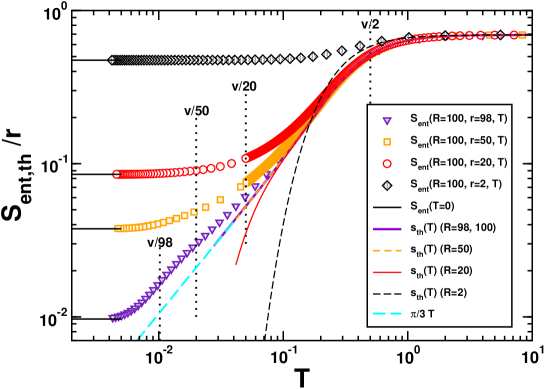
Figure 23: The finite temperature entanglement entropy per unit length of the subsystem for an $XX$ spin chain shown along with the thermal entropy for system sizes of $r=2,20,50,98$. For the entanglement entropy the total system size was $R=100$. All entropies are plotted per unit length.

As usual, let us consider a subsystem, $A$ of linear extent $r$ with the entire system, $A+B$, of size $R$. Let us also consider the subsystem $A$ decoupled from $B$. Following Gibbs, it is well known that the thermal entropy for subsystem $A$ (decoupled from $B$) can be expressed as $S_{th}=-\Tr[\rho\ln\rho]$ where $\rho=e^{-H_{A}/T}/Z$ is the thermal density matrix and $H_{A}$ is the hamiltonian describing $A$. This mixed state is expected to occur if we start with our system $A$ weakly coupled to an infinite reservoir, and then trace over the reservoir. Before performing the trace, we could regard the system as being in a pure state of system plus reservoir. On the other hand, the finite $T$ entanglement entropy, $S=-tr[\rho_{A}\ln\rho_{A}]$ is defined by beginning with the system $A+B$ in the mixed state corresponding to the thermal density matrix $e^{-(H_{A}+H_{B})/T}/Z$ and then tracing over region $B$ to obtain the reduced density matrix $\rho_{A}(T)$. Again, we could arrive at this thermal density matrix by beginning with sytem $A+B$ weakly coupled to an infinite reservoir and then tracing over the reservoir. While $S_{th}(T)$ is, by construction, independent of the coupling to $B$, the entanglement entropy $S(T)$ can clearly depend on it. We shall argue that for $T\gg v/r$ the coupling to $B$ can also be neglected when calculating $S(T)$ and the entanglement entropy $S$ will then approach $S_{th}$. Such a connection was previously noted in [26] and [113].

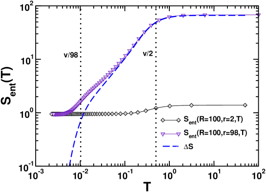
Figure 24: The finite temperature entanglement entropy for subsystems $r=2,98$ for a $R=100$ site $XX$ spin chain. At $T=0$ the two entanglement entropies are identical and the dashed line indicates the difference between the two entropies, quickly approaching 0 as $T\to 0$.

Essentially, we want to argue that we may regard region $B$ approximately as a kind of additional reservoir for region $A$ when $T$ is sufficiently large. Normally a reservoir should be sufficiently weakly coupled to the system so as not to disturb its energy eigenvalues or eigenstates. This is not true in the case of subsystem $B$ which is strongly coupled to subsystem $A$. However, this strong coupling only exists at the boundary (at the point $r$). For most eigenfunctions we can neglect the perturbation due to this coupling. The only important exception to this statement are the low energy states, with wave-lengths of order the system size and energies of O($v/r$). We can expect these to be strongly perturbed by the coupling to subsystem $B$ and consequently expect $S(T)$ to be strongly modified from the thermal entropy, $S_{th}(T)$ at low temperatures. However, when $T\gg v/r$, we expect these states to make a negligible contribution to $S(T)$ since the density of states is much larger at higher energies. Therefore we expect $S(T)$ to approach $S_{th}(T)$ when $T\gg v/r$. This argument suggests that this should occur regardless of $R$. We also expect this correspondance to hold regardless of boundary conditions. The thermal entropy for region $A$ becomes independent of whether it is calculated with pbc or obc when $T\gg v/r$. Similarly the entanglement entropy becomes independent of whether region $A$ is part of a system, $A+B$ which obeys pbc or obc at $T\gg v/r$.

In order to provide numerical evidence that $S(T)$ indeed does approach $S_{th}$, the thermal entropy, we have performed exact calculations for both quantities on an $XX$ spin chain of length $R=100$. The finite $T$ entanglement entropy is calculated for a subsystem, $A$, of size $r$ within a total system $A+B$ of size $R$ obeying periodic boundary conditions. We have also calculated the thermal entropy, $S_{th}(T)$, for a system of size $r$ also with periodic boundary conditions. We then compare $S(T)/r$ to $S_{th}(T)/r$. Our results are shown in Fig. 23 where both entropies are plotted per unit length of the subsystem. Four different sub-system sizes of $r=2,20,50,98$ are considered and in all cases do we observe excellent agreement with the thermal entropy at sufficiently high temperature. In Fig. 24 is shown the finite temperature entanglement entropy for a $R=100$ site $XX$ spin chain for two different subsystem sizes of $r=2,98$. At $T=0$ the two entanglement entropies are identical and the difference between the two is shown as the solid line, quickly approaching 0 as $T\to 0$.

Appendix F Solitons in the Majumdar-Ghosh Model

In this appendix we focus on various properties of the MG model that also can be calculated with very high precision using the TS-ansatz as described in section 6.1. We begin by a determination of $\psi^{sol}_{n}$.

F.1 Determination of $\psi^{sol}_{n}$

It is important to note that even though the thin soliton states $|n\rangle$ are linearly independent they are not orthogonal. The matrix of overlaps, $B$, is given by:

$$B_{n,m}=\langle n|m\rangle=2^{-|n-m|}.$$ (6.1)

If we now consider the action of the Hamiltonian Eq. (1.4) within the subspace spanned by the TS-states and define $H^{\prime}=H+3J{R}/8\ I$ ($I$ is the identity matrix) it can be shown that [103, 104]:

$$H^{\prime}|0\rangle \approx \frac{J}{4}\left[2|0\rangle-|1\rangle\right],\ \ n=0$$

$$H^{\prime}|n\rangle \approx \frac{J}{4}\left[\frac{5}{2}|n\rangle-|n-1\rangle-|n+1\rangle\right],\ \ n\neq 0,N_{d}$$

$$H^{\prime}|N_{d}\rangle \approx \frac{J}{4}\left[2|N_{d}\rangle-|N_{d}-1\rangle\right],\ \ n=N_{d}.$$ (6.2)

Note that $H^{\prime}$ applied to a TS-state will in general also generate a contribution that is not in the TS-subspace. Here we have dropped the part of such “fat soliton” states that is orthogonal to the TS-states since we have restricted $H^{\prime}$ to the TS-subspace. We rewrite, Eq. (6.2) in the following way:

$$H^{\prime}|n\rangle=\frac{J}{4}h^{\prime}_{nm}|m\rangle,$$ (6.3)

where $h^{\prime}_{nm}$ is a symmetric matrix with $h^{\prime}_{00}=h^{\prime}_{N_{d}N_{d}}=2$ and $h^{\prime}_{nn}=5/2$ for $n\neq 0,N_{d}$ and $h^{\prime}_{n,n+1}=h^{\prime}_{n+1,n}=-1$ for $n=1,\ldots,N_{d}-1$. Using the full hamiltonian $H$ in Eq (1.4) we can then write:

$$\frac{\langle\Psi_{TS}^{\Uparrow}|H|\Psi_{TS}^{\Uparrow}\rangle}{\langle\Psi_{TS}^{\Uparrow}|\Psi_{TS}^{\Uparrow}\rangle}=\frac{\sum_{m,n=0}^{N_{d}}\psi_{m}^{sol}A_{m,n}\psi^{sol}_{n}}{\sum_{m,n}\psi^{sol}_{m}B_{m,n}\psi^{sol}_{n}}-\frac{3}{8}J{R},$$ (6.4)

where, perhaps surprisingly, it turns out that the $A_{m,n}$ is simply given in matrix notation by $A\equiv h^{\prime}BJ/4=3JI/8$. We can now determine the $\psi_{n}^{sol}$ in a variational manner by minimizing the energy, Eq. (6.4). This is straightforward to do using the method of Lagrange multipliers and the constraint $\sum_{m,n}\psi^{sol}_{m}B_{m,n}\psi^{sol}_{n}=1$, coming from normalizing the wave-function. Due to the simple form of the matrix $A$ and the fact that the matrix $B$ has only positive definite eigenvalues, it is then seen that the optimal values for the $\psi^{sol}_{n}$ is given by the eigenvector of $B$ corresponding to the largest eigenvalue, $\lambda_{max}$. Furthermore, since $\langle H^{\prime}\rangle$ coincides with our definition of the soliton mass, we see that for open boundary conditions (obc) $\Delta_{sol}^{TS,obc}$ is given by:

$$\Delta_{sol}^{TS,obc}=\frac{3J}{8\lambda_{max}}.$$ (6.5)

For ${R}=201,401$ we find $\Delta_{sol}^{TS,obc}/J=0.12523,0.12506$, respectively, in excellent agreement with the result for periodic boundary conditions.

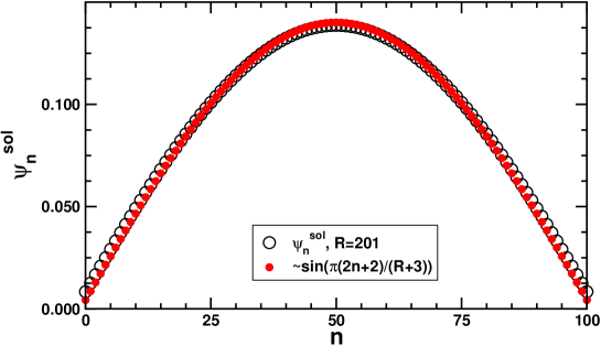
Figure 25: Variationally determined $\psi^{sol}_{n}$ (open circles) for ${R}=201$ shown with the the free particle form given by Eq. (6.5).

We note that the same $\psi^{sol}_{n}$ can be found by assuming that $\langle n|m\rangle=\delta_{n,m}$ and then solving the tight binding model resulting from Eq. (6.2). In matrix form this tight binding model will simply be given by the matrix $h^{\prime}$. However, since $h^{\prime}B$ is proportional to $I$ an eigenstate of $h^{\prime}$ is also an eigenstate of $B^{-1}$ ($B^{-1}$ exists since $B$ has positive definite eigenvalues) and then also of $B$. Hence, finding the eigenvector with lowest eigenvalue of $h^{\prime}$ will also find the eigenvector with the largest eigenvalue of $B$ and hence the optimal $\psi^{sol}_{n}$. This somewhat surprising observation, implies that at the MG-point the non-orthogonality of the thin soliton states cannot play an important role as we shall discuss in more detail later.

As an illustration we show in Fig. 25 the variationally determined $\psi^{sol}_{n}$ for ${R}=201$ along with the free particle form, Eq. (6.5). Clearly the agreement is relatively good even for this relatively small system size.

F.2 $S^{z}_{r}$ for ${R}$ odd ($J^{\prime}_{K}=1$)

We now turn to a discussion of $\langle S^{z}_{r}\rangle$ which also can be calculated employing the TS-ansatz, showing several surprising features.

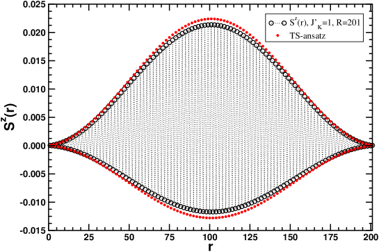
Figure 26: $\langle S^{z}_{r}\rangle$ at the MG point ($J_{2}=J/2)$ calculated using the TS-ansatz, Eq. (6.2) and variationally determined $\psi^{sol}_{n}$ for ${R}=201$ (solid circles). DMRG results for $\langle S^{z}_{r}\rangle$ at the MG point keeping $m=256$ states (open circles).

The TS-ansatz, Eq. (6.2), is constructed using the single soliton states which do not include states where the soliton is on an even site when ${R}$ is odd. It would then seem natural to assume that if we calculate $\langle S^{z}_{r}\rangle$ using the TS-ansatz it would then be zero for $r$ even. However, due to the non-orthogonality of the thin soliton states this turns out not to be the case. In fact we find that:

$$\langle\Psi_{TS}^{\Uparrow}|S^{z}_{r}|\Psi_{TS}^{\Uparrow}\rangle=\frac{\sum_{m,n=0}^{N_{d}}\psi_{m}^{sol}D_{m,n}\psi^{sol}_{n}}{\sum_{m,n}\psi^{sol}_{m}B_{m,n}\psi^{sol}_{n}},$$ (6.6)

with, for $r$ odd:

$$D_{n,m}=\left\{\begin{array}[]{cc}\frac{1}{2}2^{-|n-m|}&\ n\leq\frac{r-1}{2},m\geq\frac{r-1}{2}\\ \frac{1}{2}2^{-|n-m|}&\ m\leq\frac{r-1}{2},n\geq\frac{r-1}{2}\\ 0&\ {\rm otherwise}\end{array}\right.,$$ (6.7)

and for $r$ even

$$D_{n,m}=\left\{\begin{array}[]{cc}-\frac{1}{2}2^{-|n-m|}&\ n<\frac{r}{2},m\geq\frac{r}{2}\\ -\frac{1}{2}2^{-|n-m|}&\ m<\frac{r}{2},n\geq\frac{r}{2}\\ 0&\ {\rm otherwise}\end{array}\right..$$ (6.8)

In Fig. 26 we show results for $\langle S^{z}_{r}\rangle$ at the MG-point ($J_{2}=J/2)$ obtained using the TS-ansatz as well as numerically using DMRG methods. Fairly good agreement is observed. Notably, the TS-ansatz clearly yields a non-zero value for $\langle S^{z}_{r}\rangle$ when $r$ is even. However, longer valence bonds, not accounted for in the TS-ansatz, clearly contribute for this value of ${R}$.

We also stress that, if we use the OTS-ansatz to describe $\langle S^{z}_{r}\rangle$ we simply find $\langle S^{z}_{r}\rangle=|\psi^{sol}_{(r-1)/2}|^{2}$ for $r$ odd, 0 for $r$ even. The non-zero result for $\langle S^{z}_{r}\rangle$ for even $r$ obtained with the TS-ansatz (See Fig. 26) is then purely a result of the non-orthogonality of the TS-states.

F.3 Dimerization for ${R}$-odd from the TS-ansatz

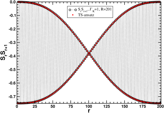
Figure 27: $\langle\vec{S}_{r}\cdot\vec{S}_{r+1}\rangle$ at the MG point ($J_{2}=J/2)$ calculated using the TS-ansatz, Eq. (6.2) and variationally determined $\psi^{sol}_{n}$ for ${R}=201$ (solid circles). DMRG results for $\langle\vec{S}_{r}\vec{S}_{r+1}\rangle$ at the MG point keeping $m=256$ states (open circles).

Finally, at the MG-point, $J_{2}=J/2$, it is also possible to obtain very precise results for the dimerization using the TS-ansatz. Most measures of the dimerization are based on the spin correlation function. We therefore consider calculations of $\langle\vec{S}_{r}\cdot\vec{S}_{r+1}\rangle$ using the TS-ansatz. With $r=2n+1$, $n=0\ldots N_{d}=({R}-1)/2$ and $B_{n,m}=2^{-|n-m|}$ we find that:

$$\langle\Psi_{TS}^{\Uparrow}|\vec{S}_{r}\cdot\vec{S}_{r+1}|\Psi_{TS}^{\Uparrow}\rangle=\frac{\sum_{m,n=0}^{N_{d}}\psi_{m}^{sol}F_{m,n}\psi^{sol}_{n}}{\sum_{m,n}\psi^{sol}_{m}B_{m,n}\psi^{sol}_{n}},$$ (6.9)

with, for $r$ odd:

$$F_{n,m}=\left\{\begin{array}[]{cc}-\frac{3}{4}2^{-|n-m|}&\ n>\frac{r-1}{2}\ {\rm or}\ m>\frac{r-1}{2}\\ 0&\ {\rm otherwise}\end{array}\right.,$$ (6.10)

and for $r$ even

$$F_{n,m}=\left\{\begin{array}[]{cc}-\frac{3}{4}2^{-|n-m|}&\ n<\frac{r}{2}\ {\rm or}\ m<\frac{r}{2}\\ 0&\ {\rm otherwise}\end{array}\right..$$ (6.11)

In Fig. 27 we show results for $\langle\vec{S}_{r}\cdot\vec{S}_{r+1}\rangle$ at the MG-point ($J_{2}=J/2)$ obtained using the TS-ansatz as well as numerically using the DMRG methods. Almost perfect agreement is observed.

References

- [1] C. H. Bennett and D. P. DiVincenzo. Nature, 404:247, 2000.
- [2] C. Holzhey, F. Larsen, and F. Wilczek. Nucl. Phys. B, 424:443, 1994.
- [3] T. J. Osborne and M. A. Nielsen. Phys. Rev. A, 66:032110, 2002.
- [4] A. Osterloh, L. Amico, G. Falci, , and R. Fazio. Nature, 416:608, 2002.
- [5] G. Vidal, J. I. Latorre, E. Rico, and A. Kitaev. Phys. Rev. Lett., 90:227902, 2003.
- [6] T.-C. Wei, D. Das amd S. Mukhopadyay, S. Vishveshwara, and P. M. Goldbart. Phys. Rev. A, 71:060305, 2005.
- [7] A. Kopp, X. Jia, and S. Chakravarty. Ann. Phys., 2006.
- [8] J. von Neumann. Gött. Nachr., 273, 1927.
- [9] A. Wehrl. Rev. Mod. Phys., 50:221, 1978.
- [10] S. Hill and W. K. Wooters. Phys. Rev. Lett., 78:5022, 1997.
- [11] W. K. Wooters. Phys. Rev. Lett., 80:2245, 1998.
- [12] C. H. Bennett, D. P. DiVincenzo, J. A. Smolin, and W. K. Wooters. Phys. Rev. A, 54:3824, 1996.
- [13] C. H. Bennett, G. Brassard, S. Popescu, B. Schumacher, J. A. Smolin, and W. K. Wooters. Phys. Rev. Lett., 76:722, 1996.
- [14] V. Vedral, M. B. Plenio, M. A. Rippin, and P. L. Knight. Phys. Rev. Lett., 78:2275, 1997.
- [15] V. Vedral and M. B. Plenio. Phys. Rev. A, 57:1619, 1998.
- [16] V. Vedral. Rev. Mod. Phys., 74:197, 2002.
- [17] M. Horodecki. Quant. Inf. Comp., 1:3, 2001.
- [18] T. J. Osborne and M. A. Nielsen. Quant. Inf. Proc., 1:45, 2002.
- [19] G. Vidal. Phys. Rev. Lett., 93:040502, 2004.
- [20] F. Verstraete and J. I. Cirac. cond-mat/0407066, 2004.
- [21] F. Verstaete and J. I. Cirac. Phys. Rev. B, 73:094423, 2006.
- [22] S. R. White. Phys. Rev. Lett., 69:2863, 1992.
- [23] U. Schollwöck. Rev. Mod. Phys., 77:259, 2005.
- [24] L. Bombelli, R. K. Koul, J. Lee, and R. D. Sorkin. Phys. Rev. D, 34:373, 1986.
- [25] M. Srednicki. Phys. Rev. Lett., 71:666, 1993.
- [26] P. Calabrese and J. Cardy. J. Stat. Mech., page 06002, 2004.
- [27] A. Kitaev and J. Preskill. Phys. Rev. Lett., 96:110404, 2006.
- [28] M. Levin and X. G. Wen. Phys. Rev. Lett., 96:110405, 2006.
- [29] P. Fendley, M. P. A. Fisher, and C. Nayak. cond-mat/0609072, 2006.
- [30] S. Furukawa and G. Misguich. cond-mat/0612227, 2006.
- [31] S. Ryu and T. Takayanagi. Phys. Rev. Lett., 96:181602, 2006.
- [32] S. Ryu and T. Takayanagi. hep-th/0605073, 2006.
- [33] S. Ghosh, T. F. Rosenbaum, G. Aeppli, and S. N. Coppersmith. Nature, 425:48, 2003.
- [34] V. Vedral. New J. Phys., 6:102, 2004.
- [35] C. Brukner, V. Vedral, and A. Zeilinger. Phys. Rev. A, 73:012110, 2006.
- [36] M. Horodecki, P. Horodecki, and R. Horodecki. Phys. Lett. A, 223:1, 1996.
- [37] B. M. Terhal. Phys. Lett. A, 271:319, 2000.
- [38] M. Lewenstein, B. Krauss, J. I. Cirac, and P. Horodecki. Phys. Rev. A, 62:052310, 2000.
- [39] A. N. Jordan and M. Büttiker. Phys. Rev. Lett., 92:247901, 2004.
- [40] G. Tóth. Phys. Rev. A, 72:010301, 2005.
- [41] L.-A. Wu, S. Bandyopadhyay, M. S. Sarandy, and D. A. Lidar. Phys. Rev. A, 72:032309, 2005.
- [42] M. Wieśniak, V. Vedral, and C. Brukner. New J. Phys., 8:258, 2005.
- [43] J. Anders, D. Kazlikowski, C. Lunkes, T. Ohshima, and V. Vedral. New J. Phys., 8:140, 2006.
- [44] T. G. Rappoport, L. Ghivelder, J. C. Fernandes, R. B. Guimarães, and M. A. Continentino. cond-mat/0608403, 2006.
- [45] T. Vértesi and E. Bene. Phys. Rev. B, 73:134404, 2006.
- [46] I. Bose and A. Tribedi. Phys. Rev. A, 72:022314, 2005.
- [47] H.-Q. Zhou, T. Barthel, J. Fjaerestad, and U. Schollwöck. cond-mat/0511732, 2005.
- [48] G. C. Levine. Phys. Rev. Lett., 93:226402, 2004.
- [49] X. Wang. Phys. Rev. E, 69:066118, 2004.
- [50] I. Peschel. J. Phys. A, 38:4327, 2005.
- [51] H. Fan, V. Korepin, V. Roychowdhury, and C. Hadley a S. Bose. cond-mat/0605133, 2006.
- [52] J. Zhao, I. Peschel I, and X.Q. Wang. Phys. Rev. B, 73:024417, 2006.
- [53] S. Y. Cho and R. H. McKenzie. Phys. Rev. A, 73:012109, 2006.
- [54] I. Affleck and A.W.W. Ludwig. Phys. Rev. Lett., 67:161, 1991.
- [55] N. Laflorencie, E. S. Sørensen, and I. Affleck. in preparation, 2007.
- [56] S. Eggert. Phys. Rev. B, 54:15590, 1996.
- [57] F. D. M. Haldane. Phys. Rev. Lett., 25:4925, 1982.
- [58] C. K. Majumdar and D. K. Ghosh. J. Phys. C, 3:911, 1969.
- [59] D. Loss and D. P. DiVincenzo. Phys. Rev. A, 57:120, 1998.
- [60] C. Simon, Y.-M. Niquet, X. Caillet, J. Eymery, J.-P. Poizat, and J.-M. Gerard. quant-phys/0609030, 2006.
- [61] M. A. Eriksson, M. Friesen, S. N. Coppersmith, R. Joynt, L. J. Klein, K. Slinker, C. Tahan, P. M. Mooney, J. O. Chu, and S. J. Koester. Quant. Inf. Proc., 3:133, 2004.
- [62] T. Costi and R. H. McKenzie. Phys. Rev. A, 68:034301, 2003.
- [63] A. O. Caldeira and A. J. Leggett. Ann. Phys., 149:374, 1983.
- [64] A. Kopp and K. Le Hur. cond-mat/0612095, 2004.
- [65] S. Lloyd. Phys. Rev. Lett., 90:167902, 2003.
- [66] S. Bose. Phys. Rev. Lett., 91:207901, 2003.
- [67] M. B. Plenio and F. L. Semião. New J. Phys., 7:73, 2005.
- [68] M. Christandl, N. Datta, A. Ekert, and A. J. Landahl. Phys. Rev. Lett., 92:187902, 2004.
- [69] D. Burgarth and S. Bose. New J. Phys., 7:135, 2005.
- [70] D. Burgarth, V. Giovannetti, and S. Bose. J. Phys. A, 38:6793, 2005.
- [71] A. Wójcik, T. Luczak, P. Kurzyński, A. Grudka, T. Gdala, and M. Bednarska. Phys. Rev. A, 72:034303, 2005.
- [72] J. Zhang, G. L. Long, W. Zhang, Z. Deng, W. Liu, and Z. Lu. Phys. Rev. A, 72:012331, 2004.
- [73] P. Karbach and J. Stolze. Phys. Rev. A, 72:030301, 2005.
- [74] J. Fitzsimons and J. Twamley. Phys. Rev. Lett., 97:090502, 2006.
- [75] E. S. Sørensen, M.-S. Chang, N. Laflorencie, and I. Affleck. J. Stat. Mech., page L01001, 2007.
- [76] P. Nozières. J. Low Temp. Phys., 17:31, 1974.
- [77] I. Affleck. Nucl. Phys. B, 336:517, 1990.
- [78] I. Affleck and A. W. W. Ludwig. Nucl. Phys. B, 352:849, 1991.
- [79] I. Affleck and A. W. W. Ludwig. Nucl. Phys. B, 360:641, 1991.
- [80] M. C. Arnesen, S. Bose, and V. Vedral. Phys. Rev. Lett., 87:017901, 2001.
- [81] D. Gunlycke, V. M. Kendon, V. Vedral, and S. Bose. Phys. Rev. A, 64:042302, 2001.
- [82] J. I. Latorre, E. Rico, and G. Vidal. Quant. Inf. Comp., 4:48, 2004.
- [83] F. Verstraete, M. A. Martin-Delgado, and J. I. Cirac. Phys. Rev. Lett., 92:087201, 2004.
- [84] H. Fan, V. Korepin, and V. Roychowdhury. Phys. Rev. Lett., 93:227203, 2004.
- [85] I. Peschel. J. Stat. Mech., page P12005, 2004.
- [86] V. Subrahmanyam. Phys. Rev. A, 69:022311, 2004.
- [87] N. Laflorencie, E. S. Sørensen, M.-S. Chang, and I. Affleck. Phys. Rev. Lett., 96:100603, 2006.
- [88] L. Amico, A. Osterloh, F. Plastina, R. Fazio, and G. M. Palma. Phys. Rev. A, 69:022304, 2004.
- [89] P. Calabrese and J. Cardy. J. Stat. Mech., page 04010, 2004.
- [90] G. De Chiara, S. Montangero, P. Calabrese, and R. Fazio. J. Stat. Mech., page P03001, 2006.
- [91] B. S. Shastry and B. Sutherland. Phys. Rev. Lett., 47:964, 1981.
- [92] B.-Q. Jin and V. E. Korepin. J. Stat. Phys., 116:79, 2004.
- [93] E. Sørensen. J. Phys. Cond. Matt., 10:10655, 1998.
- [94] G. Refael and J. E. Moore. Phys. Rev. Lett., 93:260602, 2004.
- [95] F. Alet, S. Capponi, N. Laflorencie, and M. Mambrini. cond-mat/0703027, 2007.
- [96] E. S. Sørensen and I. Affleck. Phys. Rev. B, 53:9153, 1996.
- [97] V. Barzykin and I. Affleck. Phys. Rev. B, 57:432, 1998.
- [98] V. Barzykin and I. Affleck. J. Phys. A, 32:867, 1999.
- [99] A. A. Abrikosov and A. A. Migdal. J. Low Temp. Phys., 3:519, 1970.
- [100] H. Frahm and A.A. Zvyagin. J. Cond. Matt., 9:9939, 1997.
- [101] I. S. Gradshteyn and I. M. Ryzhik. Table of Integrals, Series, and Products. Academic Press, 2000.
- [102] U. Schollwöck, Th. Jolicœur, and T. Garel. Phys. Rev. B, 53:3304, 1996.
- [103] W. J. Caspers and W. Magnus. Phys. Lett. A, 88A:103, 1982.
- [104] W. J. Caspers, K. M. Emmett, and W. Magnus. J. Phys. A, 17:2687, 1984.
- [105] E. S. Sørensen, I. Affleck, D. Augier, and D. Poilblanc. Phys. Rev. B, 58:14701, 1998.
- [106] S. W. Tsai and J. B. Marston. Phys. Rev. B, 62:5546, 2000.
- [107] S. Eggert and I. Affleck. Phys. Rev. B, 46:10866, 1992.
- [108] I. Affleck. J. Phys. A, 31:4573, 1998.
- [109] S. Rommer and S. Eggert. Phys. Rev. B, 62:4370, 2000.
- [110] M. M. Wolf. Phys. Rev. Lett., 96:010404, 2006.
- [111] D. Gioev and I. Klich. Phys. Rev. Lett., 96:100503, 2006.
- [112] T. Barthel and U. Schollwöck M.-C. Chung. cond-mat/0602077, 2006.
- [113] V. E. Korepin. Phys. Rev. Lett., 92:096402, 2004.