Entanglement entropy of the random spin-1 Heisenberg chain

Abstract

Random spin chains at quantum critical points exhibit an entanglement entropy between a segment of length $L$ and the rest of the chain that scales as $\log_{2}L$ with a universal coefficient. Since for pure quantum critical spin chains this coefficient is fixed by the central charge of the associated conformal field theory, the universal coefficient in the random case can be understood as an effective central charge. In this paper we calculate the entanglement entropy and effective central charge of the spin-1 random Heisenberg model in its random-singlet phase and also at the critical point at which the Haldane phase breaks down. The latter is the first entanglement calculation for an infinite-randomness fixed point that is not in the random-singlet universality class. Our results are consistent with a $c$-theorem for flow between infinite-randomness fixed points. The formalism we use can be generally applied to calculation of quantities that depend on the RG history in $s\geq 1$ random Heisenberg chains.

I Introduction

Understanding universal behavior near quantum critical points has been a major goal of condensed matter physics for at least thirty years. Quantum critical points describe continuous phase transitions at zero temperature, where quantum-mechanical phase coherence exists even for the long-wavelength fluctuations that control the transition. Some quantum critical points can be understood via mapping to standard classical critical points in one higher dimension, but many of the most experimentally relevant quantum critical points do not seem to fall into this category. Furthermore, even quantum critical points that can be studied using the quantum-to-classical mapping have important universal features such as frequency-temperature scaling that do not appear at finite-temperature critical points. Sachdev (1999)

One potentially universal feature of quantum critical points is the ground-state entanglement entropy, defined as the von Neumann entropy of the reduced density matrix created by a partition of the system into parts A and B:

$$S=-{\rm Tr}\ \rho_{A}\log_{2}\rho_{A}=-{\rm Tr}\ \rho_{B}\log_{2}\rho_{B}.$$ (1)

The entanglement entropy of the ground state at or near a quantum critical point can, in some cases, be understood via the quantum-to-classical mapping; an important example is that of quantum critical points in one dimension that become two-dimensional conformal field theories (CFTs), where the entanglement entropy in the quantum theory has a logarithmic divergence, whose coefficient is connected to the central charge of the classical CFT:  Holzhey et al. (1994); Vidal et al. (2003); Calabrese and Cardy (2004); Ryu and Takayanagi (2006a)

$$\lim_{N\rightarrow\infty}S\sim{c\over 3}\log_{2}N,$$ (2)

where we consider $A$ as a finite contiguous set of $N$ spins and $B$ is the complement of $A$ in the chain. Away from criticality, the entanglement $S$ is bounded above as $N\rightarrow\infty$ (the one-dimensional version of the “area law”.Srednicki (1993)) Surprisingly, the entanglement entropy, whose definition is closely tied to the lattice, is actually a universal property of the critical field theory, and hence independent of lattice details. At this time we lack a similarly complete understanding of critical points in higher dimensions; isolated solvable cases include free fermions Gioev and Klich (2006); Wolf (2006), higher dimensional conformal field theories Ryu and Takayanagi (2006a, b), and one class of $z=2$ quantum critical points.Fradkin and Moore (2006)

The connection between the central charge of CFT’s and their entanglement entropy implies that indeed for quantum critical points with classical analogs, the natural measure of universal critical entropy in the quantum system (the entanglement entropy) is determined by the standard measure of critical entropy in the classical system (the central charge). In addition, it translates important notions about the central charge to the realm of the universal quantum measure - the entanglement entropy. Zamolodchikov’s $c$-theorem Zamolodchikov (1986) states that the central charge $c$ decreases along unitary renormalization-group (RG) flows. Therefore we conclude that the entanglement entropy of CFT’s also decreases along RG flows. Stated this way, the strength of the $c$-theorem may apply to universal critical entropies in quantum systems that are not tractable by the quantum-to-classical mapping.

One such class of systems is the strongly random 1D chains with quantum critical points that can be studied by the real-space renormalization group (RSRG) technique (see Ref. Igloi and Monthus, 2005 for review). The archetype of such a system is the random Heisenberg $s=1/2$ antiferromagnet, which exhibits the “random-singlet” (RS) phase.Fisher (1994) In fact, disorder introduced to the pure Heisenberg model (which is a CFT with c=1) is a relevant perturbation, which makes it flow to the RS phase. In Ref. Refael and Moore, 2004 the disorder-averaged entanglement entropy is found to be logarithmically divergent as in the pure case, but with a different universal coefficient, which corresponds to an effective central charge ${\tilde{c}}=\ln 2$, compared to $c=1$ for the pure case. This result has been verified numerically for the random-singlet phase of the XX and XXZ chains, which are expected to have the same critical properties Laflorencie (2005); De Chiara et al. (2006).

The RS phase is but one example of an infinite randomness fixed point; special points which obey unique scaling laws. For instance, instead of energy-length scaling with $1/E\sim L^{z}$ for pure quantum-critical scaling, we have: Fisher (1994, 1995)

$$\ln 1/E\sim L^{\psi},$$ (3)

where in the RS phase, $\psi=1/2$. The infinite-randomness fixed points are, loosely speaking, the random analogs of pure CFT’s, and therefore it is important to understand all that we can about their special universal properties, such as their entanglement entropy. Generically such points can be reached as instabilities to disorder of well-known CFT’s (e.g. in the XX, Heisenberg, and transverse-field Ising model). Also, as we shall see, random gapless systems exhibit RG flow between different infinite randomness fixed points. Another motivation for the study of the entanglement entropy in these systems is to understand if they exhibit any correspondence with the pure CFT $c$-theorem. Namely, does the entanglement entropy, or a related measure, also decreases along flow lines of systems with randomness? This question can be broken into two: (a) does the entanglement entropy decrease along flows between pure CFT’s and infinite-randomness fixed points? (b) does the entanglement entropy decrease along flows between two different infinite randomness fixed points?

The first of these questions was taken up by Santachiara, Santachiara (2006) who showed that the random singlet phase of the parafermionic Potts model with $n\geq 42$ flavors has a higher entanglement entropy than the pure model. The second question, however, is still open. To answer it, and gain more insight into the entanglement entropy of random systems, we must consider systems which exhibit more complicated fixed points than the RS phase. In this paper we analyze entanglement entropy in the fixed points of the random Heisenberg spin-1 chain; particularly at its critical point where the Haldane phase breaks down (the phase diagram of the spin-1 Heisenberg chain is shown in Fig. 1), we refer to this critical point throughout as the Haldane-RS critical point. This extends our previous work by the authors and others on the entanglement entropy in a variety of “random-singlet” phases Refael and Moore (2004); Santachiara (2006); Bonesteel and Yang (2006); Igloi et al. (2007) and opens the way for a similar calculation in the more complicated $s>1$ Heisenberg chains.

The strongly random critical points of $s=1$, Hyman and Yang (1997); Monthus et al. (1998); Lin et al. (2003); Boechat et al. (1996); Saguia et al. (2002) $s=3/2$, Refael et al. (2002), and higher-spin Damle and Huse (2002) chains are random analogs of the integrable higher-spin Takhtajan-Babudjian chains.Takhtajan (1982); Babudjian (1982) Consider $s=1$ as an example: the Hamiltonian

$$H=\sum_{i}\left[\hat{\bf S}_{i}\cdot\hat{\bf S}_{i+1}-(\hat{\bf S}_{i}\cdot\hat{\bf S}_{i+1})^{2}\right]$$ (4)

is critical, while without the bi-quadratic term it would be gapped; its critical theory Affleck (1986) is referred to as the $SU(2)$ $k=2$ Wess-Zumino-Witten model, with central charge $c=3/2$. This critical theory has a relevant operator that corresponds to modifying the coefficient of the bi-quadratic term in the lattice model and thereby opening up a gap. There are similar unstable critical points in the phase diagram of higher-spin chains: although the generic higher-spin chain is either gapped (for integer spin) or gapless (for half-integer spin), there is an integrable Hamiltonian, given by a polynomial in $(\hat{\bf S}_{i}\cdot\hat{\bf S}_{i+1})$, that is gapless and critical with the central charge $c=3s/(s+1)$. These critical points have additional symmetry given by the $SU(2)$ Kac-Moody algebra at level $k=2s$.

Before plunging into the details of our calculation, let us summarize our results. We find that the leading contribution to the entanglement entropy of the spin-1 random Heisenberg model at the Haldane-RS critical point is:

$$S\sim\frac{1}{3}{c_{eff}}\log_{2}L=\frac{1}{3}\frac{4}{3}\cdot(1.3327-10^{-3})\cdot\ln 2\log_{2}L.$$ (5)

where the subtraction indicates the uncertainty in the results, which is an upper bound. The effective central-charge we find is thus:

$$c_{eff}^{(r_{c})}=1.232$$ (6)

Referring to question (a) above, $c_{eff}^{r_{c}}<3/2$, i.e., is smaller than the central charge of the corresponding pure critical point. With respect to question (b), this effective central-charge is indeed bigger than the corresponding central-charge of both the Haldane phase, which vanishes, and the spin-1 RS phase, which has:

$$c_{eff}^{s=1\,RS}=\ln 3=1.099.$$ (7)

In our work we find that the methods used for the previously studied random-singlet-like critical points are inadequate to study the spin $s>1/2$ more complicated critical points, where the history dependence of the renormalization group is more complicated. The method developed in this paper and applied to the spin-1 case provides a general approach to the entanglement entropy of random critical points in one dimension accessible by real-space renormalization group. It also presents a well developed framework for other history dependent quantities, such as correlation functions and transport properties.

The following section reviews some basic results from the physics of infinite randomness fixed points, including the higher-symmetry points that exist in random spin chains. We review the strategy of our calculation in Sec. III, and then proceed to derive the main results of this paper in sections IV-VII, where we obtain the renormalization-group history dependence for the $s=1$ chain and thereby its entanglement in a controlled approximation and estimate the accuracy of the approximation. The technique is compared to numerics for a related simplified quantity of “reduced entanglement” for which our technique provides exact results, with good agreement. In Sec. VIII we compare our results to the known value for a certain fine-tuned critical point of the pure spin-1 chain, which bears on question (a) above. We also compare the entanglement entropy at the two random fixed points of the spin-1 chain.

II Review of random-singlet and higher-spin infinite-randomness fixed points

II.1 Random-singlet phases - the simplest infinite randomness fixed points

The spin-1/2 Heisenberg chain is an antiferromagnetic chain at criticality, whose low-energy behavior is described by a conformal-field theory with central charge $c=1$. Upon introduction of disorder, the low-energy behavior of the chain flows to a different critical phase: the random-singlet phase. Fisher (1994)

The random-singlet phase has very peculiar properties. The Hamiltonian of the system is:

$$\mathcal{H}=\sum\limits_{i}J_{i}\hat{\bf S}_{i}\cdot\hat{\bf S}_{i+1}$$ (8)

Roughly speaking, the strongest bond in the chain, say, $J_{i}$, localizes a singlet between sites $i$ and $i+1$. Quantum fluctuations induce a new term in the Hamiltonian which couples sites $i-1$ and $i+2$:Ma et al. (1979); Dasgupta and Ma (1980)

$$\mathcal{H}^{\prime}_{i-1,\,i+2}=\frac{J_{i-1}J_{i+1}}{2J_{i}}\hat{\bf S}_{i-1}\cdot\hat{\bf S}_{i+2}.$$ (9)

Eq. (9) is the Ma-Dasgupta rule for the renormalization of strong bonds. Repeating this process produces singlets at all length scales, as bonds renormalize into large objects.

A useful parametrization of the couplings in the analysis of the random spin-1/2 Heisenberg chain is:

$$\beta_{i}=\ln\frac{\Omega}{J_{i}}$$ (10)

where $\Omega$ is the highest energy in the Hamiltonian:

$$\Omega={\rm max}_{i}\{J_{i}\},$$ (11)

and plays the role of a UV cutoff. It is beneficial to also define a logarithmic RG flow parameter:

$$\Gamma=\ln\frac{\Omega_{0}}{\Omega}$$ (12)

where $\Omega_{0}$ is an energy scale of the order of the maximum $J_{i}$ in the bare Hamiltonian. In terms of these variables, and using the Ma-Dasgupta rule, Eq. (9), we can construct a flow equation for the distribution of couplings $\beta_{i}$:

$$\begin{array}[]{c}\frac{dP(\beta)}{d\Gamma}={\partial P(\beta)\over\partial\beta\vspace{2mm}}\\ +P(0)\int\limits_{0}^{\infty}d\beta_{1}\int\limits_{0}^{\infty}d\beta_{2}\delta_{\left(\beta-\beta_{1}-\beta_{2}\right)}P(\beta_{1})P(\beta_{2}).\end{array}$$ (13)

Where the first term describes the reduction of $\Omega$, and the second term is the application the Ma-Dasgupta rule. For the sake of readability of equations, we denote the convolution with the cross sign:

$$P(\beta_{1})\stackrel{{\scriptstyle\beta}}{{\times}}R(\beta_{2})=\int\limits_{0}^{\infty}d\beta_{1}\int\limits_{0}^{\infty}d\beta_{2}\delta_{\left(\beta-\beta_{1}-\beta_{2}\right)}P(\beta_{1})R(\beta_{2}).$$ (14)

Eq. (13) has a simple solution, found by Fisher, which is an attractor to essentially all initial conditions and distributions: Fisher (1994)

$$P(\beta)=\frac{\chi}{\Gamma}e^{-\chi\beta/\Gamma}.$$ (15)

with $\chi=1$.

Many remarkable features of the random-singlet phase are direct results of the distribution in Eq. (15). In particular, its energy-length scaling, or, alternatively, the energy scale of a singlet with length $L$, is:

$$L^{\psi}\sim\Gamma=\ln 1/E$$ (16)

with $\psi$ being a universal critical exponent:

$$\psi=1/2.$$ (17)

II.2 Entanglement entropy in the random-singlet phase

As mentioned above, in the random singlet phase of the spin-1/2 Heisenberg chain, the entanglement entropy of a segment of length L with the rest of the chain is: Refael and Moore (2004)

$$S\sim\frac{\ln 2}{3}\log_{2}L.$$ (18)

The origin of this entanglement in the random singlet phase is simple to understand. Consider the borders of the segment $L$; the entanglement of Eq. (18) is due to singlets connecting the segment $L$ to the rest of the chain. Each singlet contributes entanglement 1, and to calculate the total entanglement we need to count the number of singlets going over one of the borders of the segment $L$. Alternatively, the entanglement is twice the number of singlets shorter than $L$ crossing a single partition (i.e., one of the barriers).

In Ref. Refael and Moore, 2004 we developed a method that allows to count this number of singlets as the RG progresses from high energy scales, in which short singlets form, up to the energy scales $\Gamma\sim L^{1/2}$, where the singlets are of the same length as the segment length. Our method strongly resembles the calculation in Ref. Fisher et al., 1999.

In this paper we will generalize this method in order to calculate the entanglement entropy of more complicated infinite-randomness fixed points in $s>1/2$ spin-chains.

The random-singlet phase can occur in the random Heisenberg model of any spin $s$, but when $s>1/2$, the randomness needs to be sufficiently strong, such that strong bonds restrict the two sites they connect to be in the complete singlet subspace. This implies that instead of entanglement 1, each singlet contributes:

$$\log_{2}(2s+1)$$

to the total entanglement. Therefore the entanglement of the spin-s random singlet phase is:

$$S\sim\frac{\ln 2\cdot\log_{2}(2s+1)}{3}\log_{2}L.$$ (19)

II.3 Higher spins infinite-randomness fixed points

The random-singlet phase, with universal distribution (15) and length-energy scaling, Eq. (16), is but one example of an infinite randomness fixed point. In general, disordered systems may have a similar type of logarithmic length-energy scaling relations, Eq. (16) with different $\psi$. This replaces the notion of the dynamical scaling exponent $z$ in $L^{z}\sim 1/E$ of pure critical points. Similarly, other infinite-randomness fixed points may exist with a different value of $\chi$ in Eq. (15), but with the same functional form of the distribution. The numbers $\psi$ and $\chi$ are the critical exponents which parametrize different infinite-randomness universality classes.

A prime example of different infinite-randomness critical fixed points comes from Heisenberg models with spin $s>1/2$. Following Refs. Monthus et al., 1998; Hyman and Yang, 1997 and Refael et al., 2002 which dealt with the spin-1 and spin-3/2 cases respectively, Damle and Huse have shown that a spin-s chain may exhibit infinite-randomness fixed points with:

$$\begin{array}[]{cc}1/\psi=2s+1,&\chi=2s.\end{array}$$ (20)

These fixed points were dubbed domain-wall symmetric fixed points for reasons that will become clear shortly.

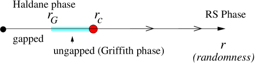
Figure 1: Phase diagram of the spin-1 random Heisenberg model. At $r=0$ the chain is in the gapped Haldane phase and its ground state resembles a valence-bond solid (VBS). As randomness is increased, the gap is destroyed at $r_{G}$, but the VBS structure survives up to the critical point, $r=r_{c}$. At $r>r_{c}$ the chain is in the spin-1 random-singlet phase. At the critical point, a different infinite randomness fixed point obtains, which has $\psi=1/2$, and $\chi=2$. We concentrate on the entanglement entropy of this point.

Figure 2: (a) At very low disorder, the ground state of the spin-1 Heisenberg chain is well described as a valence-bond solid. Each spin-1 site is described by two spin-1/2 parts (black dots) that are symmetrized. Each site forms a spin-1/2 singlet to its right and to its left. (b) As disorder grows, defects appear in the VBS structure, and the gap is suppressed. (c) At very high disorder, a phase transition occurs to the spin-1 random singlet (RS) phase.

II.4 The spin-1 Heisenberg model

This paper concentrates on the entanglement entropy of the random spin-1 Heisenberg chain at its critical point. The phase diagram of this system is shown in Fig. 1. Without disorder, the spin-1 chain has a gap (the “Haldane gap”).Haldane (1983) The ground state of the chain is adiabatically connected to the valence bond solid (VBS) of the AKLT chain, Affleck et al. (1987) in which each site forms a spin-1 singlet with both of its neighbors: (see Fig. 2a)

$$\left|\psi\right\rangle=\prod\limits_{i}\frac{1}{\sqrt{2}}\left(\hat{a}^{\dagger}_{i}\hat{b}^{\dagger}_{i+1}-\hat{b}^{\dagger}_{i}\hat{a}^{\dagger}_{i+1}\right)\left|0\right\rangle$$ (21)

where $\hat{a}^{\dagger}$ and $\hat{b}^{\dagger}$ are the creation operators for the spin-up and spin-down Schwinger bosons. Each spin-1 site can be thought of consisting of two spin-1/2 parts, symmetrized. In the VBS state it is those spin-1/2 parts that form the spin-1/2 singlet links over all bonds. These links are represented by the spin-1/2 singlet creation operator in terms of the Schwinger bosons:

$$\frac{1}{\sqrt{2}}\left(\hat{a}^{\dagger}_{i}\hat{b}^{\dagger}_{i+1}-\hat{b}^{\dagger}_{i}\hat{a}^{\dagger}_{i+1}\right).$$ (22)

As disorder increases, defects start occurring in the perfect chain of singlet links (see Fig. 2b); these defects suppress the gap, until at a certain disorder $r_{G}$ the gap vanishes, and the chain enters into a Griffiths phase.Damle (2002); Motrunich et al. (2001) In this region there is still a line of singlets connecting side to side, but no gap. When a critical disorder $r_{c}>r_{G}$ is reached, the connection between the two sides also disappears, and the Haldane phase terminates. At disorders $r>r_{c}$ the chain’s ground state is the spin-1 random-singlet state. Our goal is to calculate the entanglement entropy at $r=r_{c}$.

II.5 Entanglement entropy in the spin-1 Heisenberg model at the Haldane-RS critical point

In order to calculate the entanglement entropy in the spin-1 Heisenberg model at its intermediate-randomness critical point, we employ the real-space RG technique. This technique generalizes simply to the spin-$s>1/2$ case. As in the spin-1/2 case, the first step is to find the strongest bond in the chain. But instead of putting the strongly interacting sites in a complete singlet, we just insert one Schwinger-boson singlet (SBS) (Eq. 22) to the bonds’ wave-function. Monthus et al. (1998) Effectively, this reduces the spin of each site by 1/2, and reduces the energy of the most excited state of the bond. If disorder is very weak, the SBS’s form uniformly, and the AKLT state results. On the other hand, if the disorder is very strong, SBS’s form in pairs between strongly interacting sites, and the spin-1 random singlet phase results.

Once more, the origin of the entanglement entropy is clear; each SBS going over a partition contribute entropy of the order 1 to the entanglement between the two sides of the partition. We need to count the entanglement of these SBS’s until their length equals the size of the segment under consideration. The challenge of this calculation, however, is that each singlet going over the partition contributes an amount of entropy that depends on the singlet configuration forming both at higher and lower energies. This is due to the fact that each site can support two singlets connecting it to other sites, and therefore the ground state of the system is no longer a product state of site-pairs wave function.

Another complication in the $s=1$ case is the possibility of forming ferromagnetic bonds. This happens, for instance, if an even number of bonds localize one SBS each. The edges of this singlet chain have spin-1/2 each, which interact with each other ferromagnetically. At low energies in the RG process, this strong FM bond can be decimated, in which case the two spin-1/2 coalesce to a single spin-1. If the partition we are concerned with is between these two spin-1/2, then after the FM decimation, the partition is lodged inside a spin-1 site.

Thus to be able to calculate the entanglement entropy in $s>1/2$ spin chains, we need not only a count of the SBS going over a partition, but a full knowledge of disconnected singlet configurations: their probabilities, the energy scale at which they form, and their exact von-Neumann entanglement entropy. To carry out this calculation, we will use the domain-wall description Damle (2002); Damle and Huse (2002) of the Haldane-RS critical point.

II.6 Domain-wall picture

Our current understanding of the spin-1 critical point between the Haldane phase and the random-singlet phase relies on the Damle-Huse domain-wall picture. Let us first demonstrate this picture in terms of the spin-1/2 random singlet phase. One can think of the random-singlet phase as forming through a competition between two possible singlet domains: Domain (1,0) with singlets appearing on odd bonds only, and domain (0,1) with singlets appearing on even bonds. The notation $(a,2s-a)$ with $0\leq a\leq 2s$ signifies a domain with $a$ spin-1/2 singlet links on odd bonds, and $2s-a$ spin-1/2 singlet links on even bonds. This notation makes it easy to think about randomness as competition between different dimerizations. For each domain, there is a probability $\rho_{a}$ to be of type $(a,2s-a)$, and also, for each domain, there is a transfer matrix, which tells the probability of domain $a$ to be followed by domain $a^{\prime}$, which is $W_{aa^{\prime}}$. Note that:

$$\sum\limits_{a^{\prime}=0}^{2s}W_{aa^{\prime}}=1.$$

In the domain picture, at any finite temperature or energy scale, the non-frozen degrees of freedom (i.e., spins that were not yet decimated) lie on domain walls. Thus in the domain wall between the (1,0) and (0,1) domains, there is one free spin-1/2 site (see Fig. 3a). This free spin interacts with similar spin-1/2’s in neighboring domain walls through an interaction mediated by quantum fluctuations of the domain in between. Thus each domain of type $a$ is associated with a bond between neighboring free spins, and has a distribution of coupling $P_{a}(\beta)$, with $\beta$ defined in Eq. (10).

The renormalization of strong bonds is now described as the decimation of a domain. In the spin-1/2 chain, whenever a domain is decimated its two neighboring domains, being identical, unite to form a single large domain - a singlet appears over the domain, and connect the spins on the two domain walls. This is the Ma-Dasgupta decimation step. The random-singlet phase appears when the (1,0) and (0,1) domains have the same frequency. It is a critical point between the two possible dimerized phases associated with the two domains.

Figure 3: (a) Two domains are possible in the spin-1/2 Heisenberg model - (1,0) and (0,1). A domain wall between them gives rise to a spin 1/2 effective site. (b) In the case of a spin-1 chain, there are three possible domains: (1,1), (2,0), and (0,2), domain walls between them are effectively a spin-1/2 and spin-1 sites respectively.

In $s>1/2$ spin chains, the domain picture is richer. In the spin-1 Heisenberg chain there are three possible domains: (0,2), (1,1), and (2,0). The VBS is associated with the (1,1) phase, which has a uniform covering of the chain with spin-1/2 singlet links. On the other hand, the strong randomness random-singlet phase in this system occurs when the competing domains are (2,0) and (0,2). This is completely analogous to the spin-1/2 random singlet phase, except that the domain walls consist of free spin-1 sites (see Fig. 3b).

A general domain wall between domains $a$ and $a^{\prime}$ can be easily shown to have an effective spin:

$$S_{e}=\frac{1}{2}|a-a^{\prime}|$$ (23)

as each singlet link leaving the domain wall removes a spin-1/2 from it.

Typically, the decimation of a domain involves forming as many singlet links as possible between the two domain walls. If the two neighboring domain are identical, $a^{\prime}=a^{\prime\prime}$, then so are the domain walls, and a full singlet is formed; this is the Ma-Dasgupta decimation rule in Eq. (9). If the two domain-walls are not-identical, and interact with each other anti-ferromagnetically, singlet links forming between the two domain walls will exhaust one of the domain-wall spins, and the domain $D_{a}$ will be swallowed by the domain containing the exhausted spin.

If the two domains neighboring a strong bond are different, $a^{\prime}\neq a^{\prime\prime}$, and the interaction between the two domain-wall spins is ferromagnetic, the two spins unite into the domain wall between $D_{a^{\prime}}$ and $D_{a^{\prime\prime}}$. For example, consider a (1,1) domain with an even number of links. it has to connect between a (2,0) domain and a (0,2) domain; both domain walls will have spin-1/2. Upon decimation of the (1,1) domain, we are left with a domain wall between (2,0) and (0,2), which has a spin-1.

Indeed at the critical point between the Haldane and random-singlet phases all three domains appear with equal probability - hence the designation - permutation symmetric critical point. Since each domain appears with the same frequency at the critical point, each possible domain wall appears with the same frequency as well. Two domain walls: $(0,2)-(1,1)$ and $(2,0)-(1,1)$ are effective spin-1/2’s, whereas the third possible domain wall, $(2,0)-(0,2)$ is a spin-1. Thus, at any finite but low temperature or energy scale, 2/3 of the unfrozen degrees of freedom are effectively spin-1/2, and 1/3 are spin-1. These fractions are universal and a direct consequence of the bare spin of the model.

The analysis of the domain-theory of the spin-1 critical point is explained in Ref. Damle and Huse, 2002. The important aspects for the purpose of our calculations are the following: (1) All domains have the same bond strength distribution:

$$P_{a}(\beta)=\frac{2}{\Gamma}e^{-2\beta/\Gamma},$$ (24)

(2) each domain has an equal probability to be of any type:

$$\rho_{a}=\frac{1}{2s+1}=\frac{1}{3}$$ (25)

(this value indicates the probability after averaging over all possible neighboring domains), and (3) the transfer matrix $W_{aa^{\prime}}$ is also the same for all $a\neq a^{\prime}$:

$$W_{aa^{\prime}}=\frac{1}{2s}(1-\delta_{aa^{\prime}})=\frac{1}{2}(1-\delta_{aa^{\prime}}).$$ (26)

Eqs. (24-26) give a complete description of the spin-1 VBS-to-RS critical point. From it we can deduce the energy-length scaling properties, Eq. (16):

$$L\sim\frac{1}{\Gamma^{3}},$$ (27)

i.e.,

$$L^{1/3}\sim\ln\Omega_{0}/\Omega.$$ (28)

III Overview of the entropy calculation

Combining the above results on this permutation symmetric fixed point, in the next sections we calculate the entanglement entropy of the VBS-RS critical point. Unlike the spin-1/2 RS case, where each singlet contributes exactly entanglement 1, the spin-1 Heisenberg model can exhibit complicated singlet configuration consisting of overlapping singlet links, and even of ferromagnetic decimations.

Nevertheless, the basic principle in our calculation remains similar to the spin-1/2 calculation outlined in Ref. Refael and Moore, 2004. We can quite generally write the entanglement entropy of a segment of length $L$ as:

$$S_{L}\sim\frac{1}{3}c_{eff}\log_{2}L=2\frac{\ln\Gamma_{L}}{\overline{\ell}}\overline{S}_{total},$$ (29)

where, following Eq. (27), $\Gamma_{L}\sim L^{1/3}$ is the RG flow parameter at the length scale $L$. Literally, this expression describes the accumulation of entropy due to configurations with average entropy $\overline{S}_{total}$, which form on average when $\ln\Gamma$ changes by $\overline{\ell}$. This configurations connect the interior and of the segment to its exterior, on one of its two sides, hence the factor of $2$. The average entropy $\overline{S}_{total}$ is:

$$\overline{S}_{total}=\sum\limits_{c}p_{c}S_{c}.$$ (30)

From Eq. (29) we can infer the effective central charge:

$$c_{eff}=\frac{2\overline{S}_{total}}{\overline{\ell}}\ln 2$$ (31)

From Eqs. (29) and (30) the challenge in the calculation becomes clear. We need to find $\overline{\ell}$, the probabilities $p_{c}$ for each configuration, and the entanglement exhibited in each such configuration, $S_{c}$.

In Sec. IV we develop a scheme that calculates the possible configurational histories in the RG process, and obtains $\overline{\ell}$ as well as $p_{c}$ for all configurations. In Sec.V we define and calculate exactly a ’reduced entanglement’. This is a simple and rough measure of entanglement that is determined just by singlet counting. In Sec. V.6 we calculate this measure numerically, thus verifying the analytical calculation in Sec. IV. In Sec. VI we calculate $S_{c}$ of the various configurations. In Sec. VII we combine the pieces into the final answer.

IV Calculation of the entropy accumulation history dependence

IV.1 Approach to the history dependence

As pointed out in the introduction, one of the complications in the spin-1 entropy calculation is the fact that the entanglement of SBS’s depends on the previous and also subsequent RG steps. This arises because SBS create correlations between partially decimated spins. For this reason, to find the entanglement entropy we need to calculate the rate of formation of various finite-size correlated structures. In the following we develop a system that follows the probability and energy scale of the these structures.

Consider a partition across which we calculate the entanglement. Let us assume that we are at an intermediate stage of the RG, in which domains are long, and correlations between domain-wall spins can be neglected (these correlations decay exponentially with the domain’s length). Also, we assume that the partition-bond (the bond in which the partition is situated) was created by a Ma-Dasgupta decimation (see Eq. 9). As we shall see, the last assumption assures that entanglement from singlets that form in the ensuing RG steps is independent of the steps preceding the Ma-Dasgupta decimation.

At this point, when the partition-bond is decimated, there are three scenarios:

(1) If the partition-bond is anti-ferromagnetic (AFM), and the two domains neighboring the bond are different, then one of these domains must be the (1,1) domain (otherwise we have a (2,0) and (0,2) domains surrounding a (1,1) domain which must be ferromagnetic as discussed below). A single SBS forms over the bond and the partition, and the bond is absorbed to the (1,1) domain. Only one domain-wall spin is decimated this way, and the other survives. The entanglement of the singlet just created depends on what happens next to the undecimated spin.

(2) If the bond is ferromagnetic (FM), i.e., it corresponds to a (1,1) domain of even length between a (2,0) and (0,2) domains, the two spin-1/2 domain-wall spins coalesce to form a spin-1 effective site (a domain wall between the (2,0) and (0,2) domains) which contains the partition. Needless to say the entanglement depends on what happens to the partition-site in later stages of the RG.

(3) If the bond is AFM, but situated between two identical domains, the two domain-wall spins connected by the bond are completely decimated. The entanglement entropy of this event can only depend on the previous decimation history of these domain walls. This is the case of the Ma-Dasgupta decimation. Indeed this decimation directly follows a Ma-Dasgupta decimation as assumed above, it contributes $S_{E}=1$ between two spin-1/2’s or $S_{E}=\log_{2}3$ between two spin-1’s.

Whereas the third scenario returns the partition-bond to the starting point of the discussion, the entropy of cases (1) and (2) above will be determined by the ensuing decimation of the sites near or at the partition until a Ma-Dasgupta decimation occurs. This is a general principle for all spin-S models; once the partition-bond is freshly determined by a Ma-Dasgupta decimation, it means that all spin-excitations within the domain are gapped out, and quantum fluctuations above the gap give the suppressed Ma-Dasgupta coupling. To count the entanglement entropy we need to follow the decimation history of the partition-bond starting right after a Ma-Dasgupta decimation, until the next one.

Our calculation will follow the above lines; we will count how long it takes, in terms of the RG progression, to form various configurations between two Ma-Dasgupta decimations. Since there are three possible domains in the spin-1 Heisenberg chain, we need to consider each possible domain separately. In Ref. Damle and Huse, 2002, Damle and Huse show that at the spin-1 critical point, each of the three possible domains, $(2,0),\,(0,2),\,(1,1)$, appear with the same probability. Thus, right after a Ma-Dasgupta decimation step, the bond over our partition, has probability $1/3$ of being each of the domains. Due to right-left reflection symmetry, the contributions due to the bond being domains (2,0) and (0,2) are the same. Therefore we only need to consider two possibilities.

The main complication in our calculation is the possibility of ferromagnetic decimation steps. A FM decimation renders our partition lodged inside a spin-1 site, which is also a domain wall. Our calculation is simplified by splitting the history analysis of the partition-bond to events from a Ma-Dasgupta decimation up to the formation of a FM partition-site, and events following the partition-site formation until a Ma-Dasgupta decimation. We start by analyzing the latter.

IV.2 Note on additivity and independence of RG times

One of our goals is the calculation of the energy scales it takes uncorrelated configuration to form. As shown in Ref. Refael and Moore, 2004, probability functions of configurations should be calculated as a function of

$$\ell=\ln\Gamma/\Gamma_{0}.$$ (32)

In the next sections we will use the fact that this time $\ell$ is additive in the following sense: the RG time between the formation of a partition-site (i.e., a spin-1 site containing the partition) to a Ma-Dasgupta decimation into a partition-bond is independent of the RG history before the formation of the spin-1 partition-site. This is clear since all the information about the coupling strengths of the bonds that led to the formation of the partition-site is swallowed within the composite spin-1 site, and the ensuing decimations are only determined by bonds coupling the partition-site to the rest of the chain. Thus the RG-time it takes to go between Ma-Dasgupta decimations is the sum of the time for a partition-site to form, and for the partition-site to be decimated:

$$\ell_{MD-MD}=\ell_{MD-PS}+\ell_{PS-MD}$$ (33)

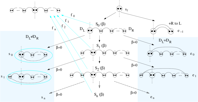
Figure 4: The possible outcomes of a spin-1 site when our partition is located inside the site. When the bond to the right (left) of the site gets decimated, it either forms a complete singlet - in case the domain to the left of the bond is the same as that to its right - or makes the spin join a (1,1) domain, in which case the bond strength has probability distribution $S_{0}(\beta)$. These two possibilities occur with the same probability, 1/2, due to the domain-wall permutation symmetry. The (1,1) domain can be decimated by forming another singlet (eventuality $e_{0}$), by forming a triplet (eventuality $s_{0}$) or by joining on its left (right) another (1,1) domain through a Ma-Dasgupta decimation (eventuality $f_{0}$). It could also form another bond to its left, giving rise to the next line of diagrams, and the eventualities $S_{1}(\beta),\,e_{1},\,s_{1},\,f_{1}$. The subscript indicates the number of bonds to the left of the partition that are involved in the (1,1) domain. Note that the $e_{n}$ and $s_{n}$ eventualities occur on a partition-bond decimation ($\beta=0$), when $D_{L}=D_{R}$ and $D_{L}\neq D_{R}$ respectively, and thus with the same probability due to domain-wall permutation symmetry ($D_{R/L}$ are the domains to right/left of the bond).

IV.3 Starting with a spin-1 site

Let us now follow the decimation process from the point that the partition is lodged inside a spin-1. We denote $s(\ell)$ as the probability of the partition to be inside an untouched spin-1 site. Due to the additivity principal, Eq. (33), we can use the boundary condition:

$$s(\ell=0)=1$$ (34)

and follow how this probability decays as the partition-site becomes correlated through SBS’s to its environment.

The possible RG histories of a spin-1 cluster with distinct entropy formation are shown in Fig. 4. Each of the eventualities in the figure has a probability distribution $S_{n}(\beta),\,e_{n},\,s_{n},\,f_{n}$, as a function of $\ell=\ln\Gamma$. Note that in the $e_{n}$ and $f_{n}$ eventualities the Ma-Dasgupta rule is applied and we get a new bond which contains the partition; at this point the spins we followed are singlet-ed out, and the entanglement of the configuration is unaffected by the subsequent RG stages. The $s_{n}$ eventualities return us to the original state of this part of the calculation, i.e., a partition contained within a site. The need to separate these eventualities by the subscript $n$, of the number of effective sites to the left (right) of the partition is necessary since configurations with different $n$’s produce different entanglement entropies.

Given the scaling form of the bond-strength distribution,

$$P(\beta)=\frac{2}{\Gamma}\exp(-2\beta/\Gamma),$$ (35)

we can now calculate exactly the probability evolution of all eventualities. First, the probability $s_{\ell}$ will diminish due to decimations of bonds on either of its sides:

$$\frac{ds(\ell)}{d\Gamma}=-2P(0)s(\ell).$$ (36)

and recall that $\ell$ and $\Gamma$ are related by Eq. (32).

Starting with $e_{-1}$, the immediate-singlet eventuality:

$$\frac{de_{-1}(\ell)}{d\Gamma}=\frac{1}{2}s_{\ell}P(0).$$ (37)

The interpretation of this equation is that the change in probability of the $e_{-1}$ eventuality, is $P(0)d\Gamma$ - the probability that the bond to the right (left) is decimated, times the probability that the domains to the left and right of the bond are the same, which is $1/2$, times the probability of the initial configuration, $s_{\ell}$. Upon substituting $P(0)$ we obtain:

$$\frac{de_{-1}(\ell)}{d\ell}=s_{\ell}.$$ (38)

If the bond to the right (left) of the partition connects to a (1,1) domain, then the spin joins a long (1,1) domain to its right (left). This domain has coupling strength $\beta$ between its walls, and hence this eventuality is characterized by the distribution: $S_{0}(\beta)$. This distribution can evolve under the RG due to decimations of other bonds to the right (left) of the partition, where the (1,1) domain is. But any decimation of its neighboring bonds will remove probability from $S_{0}(\beta)$, as will a Ma-Dasgupta decimation of the bond on which the partition sits, in the case of $\beta=0$. Thus the flow equation for $S_{0}(\beta)$ is:

$$\frac{dS_{0}(\beta)}{d\Gamma}={\partial S_{0}(\beta)\over\partial\beta}+\frac{1}{2}P(0)(S_{0}(\beta)+P(\beta_{1})\stackrel{{\scriptstyle\beta}}{{\times}}S_{0}(\beta_{2}))-2P(0)S_{0}(\beta)+\frac{1}{2}s_{\ell}P(0)P(\beta).$$ (39)

The last term represents what happens when the bond to the right (left) of the partition site is decimated, and the second-nearest domain is (1,1), which happens with probability $1/2$, hence the factor of $1/2$. The second-to-last term describes the removal of probability due to decimations on either side of the partition-bond after it was formed. The brackets describe what happens when the bond to the right (left) of the partition-bond is decimated. The two factors of $1/2$ in the brackets are the probability of the second-nearest domain on the right (left) being different than (1,1) in the first term, and (1,1) in the second term. The first term on the RHS describes the reduction of the energy scale $\Omega$. The cross denotes convolution, as defined in Eq. (14).

But a decimation to the left (right) of the partition can have two outcomes - if the bond to the left (right) is connecting the (1,1) domain of the partition with another (1,1) domain to its left (right), then a decimation of this bond means applying the Ma-Dasgupta decimation, and we can stop following the RG; this is $f_{0}$ outcome, and its evolution is:

$$\frac{df_{0}(\ell)}{d\Gamma}=\frac{1}{2}P(0)\int\limits_{0}^{\infty}d\beta S_{0}(\beta).$$ (40)

Alternatively, if the second-nearest domain to the left (right) is not (1,1), then a decimation of the bond to the left will create another spin-1/2 singlet over it, and will lead to the distribution $S_{1}(\beta)$. $S_{1}(\beta)$ has the same structure of the flow equation, except for the source term, which is now fed from $S_{0}$, rather than $s_{\ell}$:

$$\frac{dS_{1}(\beta)}{d\Gamma}={\partial S_{1}(\beta)\over\partial\beta}+\frac{1}{2}P(0)(S_{1}(\beta)+P(\beta_{1})\stackrel{{\scriptstyle\beta}}{{\times}}S_{1}(\beta_{2}))-2P(0)S_{1}(\beta)+\frac{1}{2}P(0)S_{0}(\beta).$$ (41)

again the factor of $1/2$ in the source term is due to the probability of the second-nearest domain on the left not being (1,1).

Going back to $S_{0}(\beta)$, when the bond on the partition is strong, it gets decimated. If the two neighboring domains are the same, then we apply the Ma-Dasgupta rule once $\beta=0$, in which case we obtain the singlet-ed cluster $e_{0}$. The evolution of this probability is:

$$\frac{de_{0}(\ell)}{d\Gamma}=\frac{1}{2}S_{0}(0).$$ (42)

where the factor of $1/2$ is the probability that the two neighboring domains are the same. If they are different, a new spin-1 site is born, which is eventuality $s_{0}$. It is easy to see that:

$$\frac{ds_{0}}{d\Gamma}=\frac{de_{0}}{d\Gamma}.$$ (43)

Note that we ignore what happens to the resulting new spin-1 configurations; subsequent RG of this configurations are the same as those considered in this section, and can be analyzed self-consistently.

Eq. (43) completes the consideration of all first-level eventualities. It is easy to see that Eqs. (40) - (43) generalize to the case of starting with $S_{n}(\beta)$, which is the distribution of a bond with $n$ singlets to its left (right), and a long (1,1) domain to its right (left). Thus the equations for $f_{n},\,e_{n},\,s_{n}$ become:

$$\begin{array}[]{c}\frac{df_{n}(\ell)}{d\Gamma}=\frac{1}{2}P(0)\int\limits_{0}^{\infty}d\beta S_{n}(\beta),\vspace{2mm}\\ \frac{dS_{n}(\beta)}{d\Gamma}={\partial S_{n}(\beta)\over\partial\beta}+\frac{1}{2}P(0)(S_{n}(\beta)+P(\beta_{1})\stackrel{{\scriptstyle\beta}}{{\times}}S_{n}(\beta_{2}))-2P(0)S_{n}(\beta)+\frac{1}{2}P(0)S_{n-1}(\beta),\vspace{2mm}\\ \frac{de_{n}(\ell)}{d\Gamma}=\frac{1}{2}S_{n}(0),\vspace{2mm}\\ \frac{ds_{n}}{d\Gamma}=\frac{de_{n}}{d\Gamma}.\end{array}$$ (44)

Before solving all equations, we note that the hardest part of solving Eqs. (40)-(44) is finding the distributions $S_{n}(\beta)$. Here, an important simplification occurs: Eqs. (39) and (44) for $S_{n}$ always admit a solution of the form:

$$S_{n}(\beta)=\alpha_{n}P(\beta).$$ (45)

Substituting Eq. (45) in the equation for $S_{n}$ gives:

$$\begin{array}[]{c}\frac{d\alpha_{0}}{d\Gamma}=-4\frac{\alpha_{0}}{\Gamma}+\frac{1}{2}P(0)s_{\ell},\vspace{2mm}\\ \frac{d\alpha_{n}}{d\Gamma}=-4\frac{\alpha_{n}}{\Gamma}+\frac{1}{2}P(0).\alpha_{n-1}\end{array}$$ (46)

Note that $\int\limits_{0}^{\infty}d\beta S_{n}(\beta)=\alpha_{n}$.

Starting with Eq. (36) it is easy to see that:

$$\Gamma\frac{ds_{\ell}}{d\Gamma}=\frac{ds_{\ell}}{d\ell}=-4s_{\ell}$$ (47)

and:

$$s_{\ell}=e^{-4\ell}.$$ (48)

$e_{-1}$ is immediately obtained as:

$$e_{-1}=\frac{1}{4}\left(1-e^{-4\ell}\right)$$ (49)

Note that this is the probability for a double singlet forming to the left, and the same probability applies to singlet-formation to the right. Hence the total probability of a double singlet forming is $1/2$.

Next is $\alpha_{0}$:

$$e^{4\ell}\alpha_{0}=\int\limits_{0}^{\ell}e^{4\ell}s_{\ell}$$ (50)

In fact, Eq. (46) is:

$$e^{4\ell}\alpha_{n}=\int\limits_{0}^{\ell}d\ell e^{4\ell}\alpha_{n-1}$$ (51)

It is thus helpful to define:

$$\tilde{\alpha}_{n}=e^{4\ell}\alpha_{n}.$$ (52)

In terms of the $\tilde{\alpha}$ we have:

$$\begin{array}[]{c}\tilde{\alpha}_{0}=\int\limits_{0}^{\ell}d\ell 1=\ell\vspace{2mm}\\ \tilde{\alpha}_{n}=\int\limits_{0}^{\ell}d\ell\tilde{\alpha}_{n-1}=\frac{1}{(n+1)!}\ell^{n+1}\end{array}$$ (53)

From here we can find all other eventualities. The right-leaning singlet clusters $e_{n}$ probabilities are:

$$s_{n}=f_{n}=e_{n}=\int_{0}^{\ell}d\ell e^{-4\ell}\frac{l^{n+1}}{(n+1)!},$$ (54)

for $n\geq 0$, which is extremely simple considering the tortuous way to here. The final bin probability to end up in, say, bin $e_{n}$ is:

$$e_{n}|_{\ell\rightarrow\infty}=\int_{0}^{\infty}d\ell e^{-4\ell}\frac{l^{n+1}}{(n+1)!}=\frac{1}{4^{n+2}}.$$ (55)

The sum of all $e_{n}$ eventualities is:

$$\sum\limits_{n=0}^{\infty}e_{n}=\sum\limits_{n=0}^{\infty}\frac{1}{4^{n+2}}=\frac{1}{12}$$ (56)

This is the probability to end up as a right-leaning singlet cluster. The same calculation applies to the s-bins and f-bins. Indeed - $6\times\frac{1}{12}=1/2$, which completes the probability of $2e_{-1}$ to 1. Note that the total probability of the spin-1 surviving and becoming a new spin-1 is the total $s_{n}$ sum, which is also $1/6$.

The $RG$ time of the process follows directly from the above discussion. Let us calculate the total time it takes for a spin-1 to be completely eliminated. This we do in a self consistent way: The time it takes to get completely decimated from the $s_{n}$ outcomes, is the same as the total RG time we are seeking. Thus:

$$\overline{\ell}_{1}=2\int de_{-1}\cdot\ell+2\sum\limits_{n=0}^{\infty}\int(df_{n}+de_{n})\cdot\ell+2\sum\limits_{n=0}^{\infty}\int ds_{n}\cdot(\ell+\overline{\ell}_{1})$$ (57)

where the factor of 2 is due to the reflection symmetry of the configuration enumeration. Upon use of the definitions of $e_{n},\,f_{n},\,s_{n}$ we have:

$$\frac{5}{6}\overline{\ell}_{1}=2\int_{0}^{\infty}e^{-4\ell}\ell d\ell+6\int_{0}^{\infty}e^{-4\ell}\sum\limits_{n=0}^{\infty}\frac{\ell^{n+2}}{(n+1)!}\vspace{2mm}\\ =\frac{1}{8}+6\int_{0}^{\infty}e^{-4\ell}\ell\left(e^{\ell}-1\right)=\frac{1}{8}+\frac{6}{9}-\frac{6}{16}=\frac{5}{12}$$ (58)

Hence:

$$\overline{\ell}_{1}=\frac{1}{2}$$ (59)

This is the RG time for a spin-1 partition-site to be decimated completely, and form an uncorrelated partition-bond.

IV.4 Getting from a (2,0) domain to a spin-1 site

A more complicated analysis is required for the calculation of the history of a partition-bond between a Ma-Dasgupta decimation and the formation of a spin-1 partition-site. We must consider two possibilities: first, the bond being a (2,0) or (0,2) domain, or second, being a (1,1) domain. The latter is simpler, hence we start with the former.

Right after a Ma-Dasgupta decimation, the bond distribution $R(\beta)$ is quite different from $P(\beta)$. It is actually the convolution of $P(\beta)$ with itself:

$$\begin{array}[]{c}Q(\beta)=P(\beta_{1})\stackrel{{\scriptstyle\beta}}{{\times}}P(\beta_{2})\vspace{2mm}\\ =\int\limits_{0}^{\infty}d\beta_{1}\int\limits_{0}^{\infty}d\beta_{2}P(\beta_{1})P(\beta_{2})\delta_{(\beta_{1}+\beta_{2}-\beta)}=\frac{4}{\Gamma^{2}}\beta e^{-2\beta/\Gamma}\end{array}$$ (60)

As the RG progresses, this distribution may rebound to be closer to $P(\beta)$. The flow equation it obeys is:

$$\frac{dR(\beta)}{d\Gamma}={\partial R(\beta)\over\partial\beta}+2\cdot P(0)\frac{1}{2}P(\beta_{1})\stackrel{{\scriptstyle\beta}}{{\times}}R(\beta_{2})-P(0)R(\beta).$$ (61)

The second term represents the probability that a bond on either of the two sides (hence the factor 2) gets decimated (hence $P(0)$). If the two bonds right next to the decimated bond are different (probability half), then nothing happens to the bond on the partition - the decimated bond either forms a new spin-1, or connects a (1,1) domain to a spin on the side of the partition. But if the domains near the decimated-side bonds are the same (probability $1/2$ as well), we get a Ma-Dasgupta decimation that involves the partition bond, hence the convolution. In this case, we also need to remove the original probability from the distribution $R(\beta)$, which is the origin of the last term.

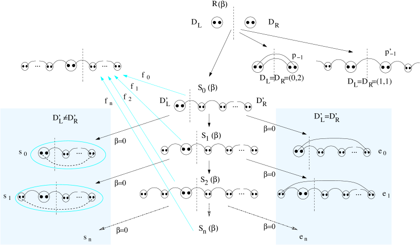
Figure 5: The possible outcomes of a partition bond of domain (2,0). When the partition-bond gets decimated, and it is between two identical domains, $D_{L}=D_{R}$, then the Ma-Dasgupta rule is applied, Depending on whether $D_{L}=D_{R}=(1,1)$ or not, eventualities $p_{-1},\,p^{\prime}_{-1}$ are obtained. If $D_{L}\neq D_{R}$, when the partition-bond gets decimated it joins a (1,1) domain, in which case the bond strength has probability distribution $S_{0}(\beta)$. The (1,1) domain can be decimated by forming another singlet (eventuality $e_{0}$), by forming a triplet (eventuality $s_{0}$) or by joining on its left (right) another (1,1) domain through a Ma-Dasgupta decimation (eventuality $f_{0}$). It could also form another bond to its left, giving rise to the next line of diagrams, and the eventualities $S_{1}(\beta),\,e_{1},\,s_{1},\,f_{1}$. The subscript indicates the number of bonds to the left of the partition that are involved in the (1,1) domain. Note that the $e_{n}$ and $s_{n}$ eventualities occur when $D_{L}=D_{R}$ and $D_{L}\neq D_{R}$ respectively, and thus with the same probability due to domain-wall permutation symmetry ($D_{R/L}$ are the domains to right/left of the bond).

The solution of Eq. (61) is straightforward, since $R(\beta)$ lives in the functional space spanned by $P(\beta)$ and $Q(\beta)$. If we write:

$$R(\beta)=a_{\ell}P(\beta)+b_{\ell}Q(\beta),$$ (62)

we obtain:

$$\frac{d}{d\ell}\left(\begin{array}[]{c}a_{\ell}\vspace{2mm}\\ b_{\ell}\end{array}\right)=\left(\begin{array}[]{cc}-3&2\vspace{2mm}\\ 1&-2\end{array}\right)\left(\begin{array}[]{c}a_{\ell}\vspace{2mm}\\ b_{\ell}\end{array}\right)$$ (63)

The eigenvalues and eigenvectors of the matrix on the RHS are:

$$\begin{array}[]{cc}-1&(1,1)\vspace{2mm}\\ -4&(2,-1)\end{array}$$ (64)

Given that the initial conditions are $a_{\ell=0}=0,\,b_{\ell=0}=1$, we obtain:

$$\begin{array}[]{c}a_{\ell}=\frac{2}{3}\left(e^{-\ell}-e^{-4\ell}\right)\vspace{2mm}\\ b_{\ell}=\frac{1}{3}\left(2e^{-\ell}+e^{-4\ell}\right)\end{array}$$ (65)

From here on, we can follow the same procedure as Sec. IV.3. The first thing to consider is having the partition-bond be decimated, with the same domains on its sides. This invokes the Ma-Dasgupta rule, terminates this step, and begins a new cycle. The differential probability of this happening is $\frac{1}{2}R(0)d\Gamma$. But there are two sub-possibilities: the neighboring domains could be either (1,1), or (2,0)/(0,2), each with probability $1/2$. The first feeds into $p^{\prime}_{-1}$, and the second to $p_{-1}$. So we obtain:

$$\begin{array}[]{c}\frac{dp_{-1}}{d\Gamma}=\frac{dp^{\prime}_{-1}}{d\Gamma}\vspace{2mm}\\ =\frac{1}{4}R(0)=\frac{1}{4}\frac{2}{\Gamma}\frac{2}{3}\left(e^{-\ell}-e^{-4\ell}\right)\end{array}$$ (66)

Thus:

$$\frac{dp_{-1}}{d\ell}=\frac{dp^{\prime}_{-1}}{d\ell}=\frac{1}{3}\left(e^{-\ell}-e^{-4\ell}\right)$$ (67)

and:

$$p_{-1}=p^{\prime}_{-1}=\frac{1}{3}\left(1-e^{-\ell}-\frac{1}{4}(1-e^{-4\ell})\right)$$ (68)

and as $\ell\rightarrow\infty$, we have:

$$p_{-1}|_{\ell\rightarrow\infty}=p^{\prime}_{-1}|_{\ell\rightarrow\infty}=\frac{1}{4}$$ (69)

So with probability $1/2$, our bond gets decimated via a Ma-Dasgupta rule right away.

The alternative possibilities arise from the case of the partition bond being decimated while its neighboring domains are different from each other - which happens with probability $1/2$. In this case the partition bond joins a (1,1) domain to its right or to its left, each with another probability factor of $1/2$. When this happens, we need to follow a distribution, $S_{0}(\beta)$, which has the same meaning and flow equation as $S_{0}(\beta)$ from Sec. IV.3, except for the source term, which is now $\frac{1}{4}R(0)P(\beta)$ (the $P(\beta)$ arises since it is the distribution of the (1,1) domain to which the partition-bond annexes):

$$\frac{dS_{0}(\beta)}{d\Gamma}={\partial S_{0}(\beta)\over\partial\beta}+\frac{1}{2}P(0)(S_{0}(\beta)+P(\beta_{1})\stackrel{{\scriptstyle\beta}}{{\times}}S_{0}(\beta_{2}))-2P(0)S_{0}(\beta)+\frac{1}{4}R(0)P(\beta)$$ (70)

As in Sec. IV.3, once the partition enters the distribution $S_{0}(\beta)$ three possibilities for termination of this stage exist: (1) form a singlet configuration via the $e_{n}$ route, (2) be involved in a Ma-Dasgupta decimation with the bond to the opposite side of the (1,1) domain - $f_{n}$ route, and (3) the partition-bond can be decimated while its neighboring domains are different, giving rise to a spin-1 containing the partition - the $s_{n}$ route. Also, $S_{0}(\beta)$ can flow into the additional $S_{n}(\beta)$ just as before.

It is easy to see that the flow equations for $e_{n},\,f_{n},\,s_{n}$ and $S_{n}(\beta)$ are the same as Eqs. (44). The only difference is $S_{0}(\beta)$, due to its different source term. Let us solve $S_{0}(\beta)$ for this case. Here too, we can write $S_{0}(\beta)=\alpha_{0}(\ell)P(\beta)$. Once we substitute this into Eq. (70), we obtain:

$$\frac{d\alpha_{0}}{d\ell}=-4\alpha_{0}+\frac{1}{2}\frac{2}{3}(e^{-\ell}-e^{-4\ell})$$ (71)

As before, it is beneficial to follow $\tilde{\alpha}_{0}=e^{4\ell}\alpha_{0}$. This obeys:

$$\frac{d\tilde{\alpha}_{0}}{d\ell}=\frac{1}{3}(e^{3\ell}-1).$$ (72)

The next step is to find $\tilde{\alpha}_{n}$, which are the probability ’amplitudes’ of $S_{n}(\beta)$, as in Eq. (45). They obey Eq. (52). As it turns out, it is helpful to expand the exponent in Eq. (72) into a power-law. Upon integration we obtain:

$$\tilde{\alpha}_{0}=\frac{1}{3}\sum\limits_{j=1}^{\infty}\frac{1}{3}\frac{(3\ell)^{j+1}}{(j+1)!}.$$ (73)

from which we can immediately find:

$$\tilde{\alpha}_{n}=\frac{1}{3}\sum\limits_{j=1}^{\infty}\frac{1}{3^{n+1}}\frac{(3\ell)^{j+n+1}}{(j+n+1)!}=\frac{1}{3^{n+2}}(e^{3\ell}-\sum\limits_{j=0}^{n+1}\frac{(3\ell)^{j}}{j!})$$ (74)

From this result we can find $e_{n}=f_{n}=s_{n}$ as a function of $\ell$:

$$\frac{de_{n}}{d\ell}=\tilde{\alpha}_{n}e^{-4\ell}$$ (75)

and hence:

$$e_{n}(\ell)=\int\limits_{0}^{\ell}d\ell\frac{1}{3^{n+2}}\left(e^{-\ell}-e^{-4\ell}\sum\limits_{j=0}^{n+1}\frac{(3\ell)^{j}}{j!}\right)$$ (76)

If we carry the integration to $\ell\rightarrow\infty$ we obtain:

$$\begin{array}[]{c}e_{n}(\infty)=\frac{1}{3^{n+2}}\left(1-\frac{1}{4}\sum\limits_{j=0}^{n+1}\left(\frac{3}{4}\right)^{j}\right)\vspace{2mm}\\ =\frac{1}{3^{n+2}}\left(1-\frac{1}{4}\frac{1-(3/4)^{n+2}}{1-3/4}\right)\vspace{2mm}\\ =\frac{1}{4^{n+2}}\end{array}$$ (77)

The sum over all $e_{n}$ is just:

$$\sum\limits_{n=0}^{\infty}e_{n}=\frac{1}{16}\frac{1}{1-1/4}=\frac{1}{12}$$ (78)

just as before.

We are now ready to calculate RG times. The total RG time for this stage, between a Ma-Dasgupta decimation and the formation of a partition-site is:

$$\overline{\ell}_{0}=2\int dp_{-1}\cdot\ell+6\sum\limits_{n=0}^{\infty}\int de_{n}\cdot\ell=\frac{2}{3}(1-\frac{1}{16})+6\sum\limits_{n=0}^{\infty}\int\limits_{0}^{\infty}d\ell\cdot\ell e^{-4\ell}\tilde{\alpha}_{n}$$ (79)

As it turns out, we can carry out the sum over $\tilde{\alpha}_{n}$ directly:

$$\begin{array}[]{c}\sum\limits_{n=0}^{\infty}\tilde{\alpha}_{n}=\sum\limits_{n=0}^{\infty}\left(\frac{e^{3\ell}}{3^{n+2}}-\sum\limits_{j=0}^{n+1}\frac{(3\ell)^{j}}{j!}\right)\vspace{2mm}\\ =\frac{1}{6}e^{3\ell}-\frac{1}{3}\sum\limits_{j=0}^{\infty}\sum\limits_{n=j-1}^{\infty}\frac{1}{3^{n+1}}\frac{(3\ell)^{j}}{j!}+1/3\vspace{2mm}\\ =\frac{1}{6}e^{3\ell}-\frac{1}{2}e^{\ell}+\frac{1}{3}.\end{array}$$ (80)

And thus:

$$\overline{\ell}_{0}=\frac{2}{3}(1-\frac{1}{16})+6\int\limits_{0}^{\infty}d\ell\ell\left(\frac{1}{6}e^{3\ell}-\frac{1}{2}e^{\ell}+\frac{1}{3}\right)=\frac{5}{8}+1-\frac{1}{3}+\frac{1}{8}=\frac{17}{12}.$$ (81)

This is the average time it takes to become either a Ma-Dasgupta decimated bond, or a spin-1 containing the partition (probability $1/6$).

IV.5 Getting from a (1,1) domain to a spin-1 site

A fresh partition-bond of a (1,1) domain can terminate either through the formation of a full singlet, or by the formation of a spin-1 partition-site (Fig. 6).

Figure 6: The possible outcomes of a partition bond of domain (1,1). When the partition-bond gets decimated, if it is between two identical domains, $D_{L}=D_{R}$, then the Ma-Dasgupta rule is applied, otherwise, it forms a partition-spin-1.

As in Sec. IV.4, we first find the flow equation for the distribution $R(\beta)$ of the partition-bond right after decimation:

$$\frac{dR(\beta)}{d\Gamma}={\partial R(\beta)\over\partial\beta}+2\cdot P(0)\left(\frac{1}{2}P(\beta_{1})\stackrel{{\scriptstyle\beta}}{{\times}}R(\beta_{2})+\frac{1}{2}R(\beta)\right)-2P(0)R(\beta).$$ (82)

Note that there are two differences with respect to the analog Eq. (61) in Sec. IV.4. The brackets contain another term $\frac{1}{2}R(\beta)$, which arises from the possibility of a bond to either side of the partition-bond being decimated, but with a different domain on its other side. This will extend the (1,1) domain of the partition-bond, but will maintain its strength. The other difference is the factor of 2 in the last term - this change is due to the fact that now any decimation of a bond neighboring the partition bond leads to its renormalization. In spite of these differences, the two additions cancel, and we obtain exactly the same result for $R(\beta)$ as in Eqs. (62) and (65).

All that remains is to find the dependencies of the two probabilities $e$ and $s$ on $\ell$, where $e$ is the probability of the partition-bond being decimated with its domains being the same on both sides, and $s$ is the probability of being decimated with different domains surrounding the partition bond, and hence forming a spin-1 (see Fig. 6). It easy to see that these probabilities are equal, and that:

$$\frac{de}{d\Gamma}=\frac{1}{2}R(0)=\frac{1}{\Gamma}\frac{2}{3}(e^{-\ell}-e^{-4\ell})$$ (83)

and hence:

$$s(\ell)=e(\ell)=\frac{2}{3}(1-e^{-\ell}-\frac{1}{4}(1-e^{-4\ell}))$$ (84)

as $\ell\rightarrow\infty$ we indeed obtain $s(\infty)=e(\infty)=1/2$.

The RG-time for this stage, i.e., between a Ma-Dasgupta decimation and the decimation of the partition bond (either FM or AFM), is:

$$\overline{\ell}_{11}=2\int de\cdot\ell=2\int\limits_{0}^{\infty}d\ell\cdot\ell\cdot\frac{2}{3}(e^{-\ell}-e^{-4\ell})=\frac{4}{3}\left(1-\frac{1}{16}\right)=\frac{5}{4}.$$ (85)

Note that now the probability of becoming a spin-1 (s eventuality) is 1/2.

IV.6 Total average time

The average total RG time between two Ma-Dasgupta decimation is given as the sum of all the time of the limited histories times their probabilities. For instance, the total time it takes for a partition-bond which is a (1,1) domain to be completely eliminated is:

$$\ell_{(1,1)}=\overline{\ell}_{11}+\frac{1}{2}\overline{\ell}_{1}=\frac{5}{4}+\frac{1}{4}=\frac{3}{2}$$ (86)

The last term is the product of the probability of forming a partition-site, and the time for this spin-1 to be completely decimated. We use the results from Eqs. (59) and (85).

A similar result applies to the (2,0) or (0,2) initial domains:

$$\ell_{(2,0)}=\ell_{(0,2)}=\overline{\ell}_{0}+\frac{1}{6}\overline{\ell}_{1}=\frac{17}{12}+\frac{1}{6}\cdot\frac{1}{2}=\frac{3}{2}$$ (87)

where we also use Eq. (81). Since this result is the same as for the (1,1) domain, the total average RG-time is:

$$\ell_{total}=\frac{3}{2}.$$ (88)

This number should be compared to the RG time between Ma-Dasgupta decimations in the random-singlet phase, which is:

$$\ell_{total}^{RS}=3.$$ (89)

Note also that this calculation is a generalized return-to-the-origin probability.

V Reduced entropy of the spin-1 chain

After analyzing the history dependence and probabilities of the various singlet configurations, what remains is the analysis of the amount of quantum entanglement in them. Because of the complexity of the quantum entanglement of SBS configurations due to the correlations they produce, it is helpful to define a measure of entanglement which neglects these short range correlations. Such a measure would be a direct count of the number of singlets that connect the two parts of our chain, and can be calculated exactly. In this section we define this reduced entanglement entropy, $E$, analyze its properties, and calculate it both analytically, and in Sec. V.6 numerically, thus verifying our analytical calculation.

V.1 Definition of the reduced entropy

The ground state of the random spin-1 Heisenberg model is constructed through iterative decimations of strong AFM and FM bonds. The reduced entanglement with respect to a partition is defined as follows: An SBS connecting between one side of the partition to the other contributes reduced-entropy of 1. Some spin-1 sites are clusters that are the result of the decimation of a FM bond. If the partition is contained within such a cluster, a SBS that connects the partition site with the sites to its right contributes a fraction $\sigma$ to the reduced entropy, and an SBS to its left contributes a fraction $1-\sigma$.

$\sigma$ is supposed to capture the internal structure of the spin-1 partition-site, and in principle may vary from cluster to cluster. When two clusters combine, their weight $\sigma$ should be the average of their weights, $\sigma_{12}=\frac{1}{2}(\sigma_{1}+\sigma_{2})$. But using reflection symmetry of the problem, we now show that we can set

$$\sigma=1/2$$ (90)

without loss of generality. Every time that an SBS forms between a partition-spin-1 to a site on the right, we would have $E=\sigma$ per singlet. But because of the reflection symmetry of the problem we also need to consider the reflected configuration, which would have $E=(1-\sigma)$ per singlet. The average of these contributions is $1/2$, independent of $\sigma$. Thus, for simplicity, we set $\sigma=1/2$.

Since the reduced entropy $E$ neglects correlations between the spin-1/2’s degrees of freedom connected by the SBS’s, it is a purely additive quantity: the reduced entanglement of a configuration is the sum of the reduced entanglement of the individual singlets.

V.2 Reduced entropy of a partition-site-1

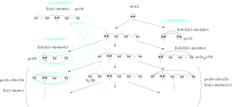
Figure 7: Starting with a partition-spin-1, the various possibilities are illustrated on the same chart as Fig. 4. $\sigma$ is the effective weight of the partition spin-1 that we begin with. Note that we omit here the future reduced entanglement in the case of the resulting partition-spin-1.

We start our analysis with a calculation of the average reduced entanglement of configurations that result from a partition site. Once we obtain our result for this intermediate stage we will consider the average reduced entanglement of the beginning stages from a Ma-Dasgupta decimation up to the formation of the spin-1 partition site.

The entropy contribution and probabilities of a partition-spin-1 are illustrated in Fig. 7. The average contributions for this stage, and its futures are (going from right to left in the figure):

$$\begin{array}[]{c}E_{1}=\vspace{2mm}\\ \frac{1}{2}\cdot 1+\frac{1}{8}\cdot 1+\left(\frac{1}{6}-\frac{1}{8}\right)\cdot 2+\frac{1}{6}\cdot 1+\frac{1}{8}\cdot\frac{1}{2}\vspace{2mm}\\ +\left(\frac{1}{6}-\frac{1}{8}\right)\cdot 1+\frac{1}{6}E_{1}\end{array}$$ (91)

where the last term self consistently adds the probability of forming a partition-spin-1, which is $1/6$, and it having the same entropy $E_{1}$. We get:

$$E_{1}=\frac{47}{40}.$$ (92)

V.3 Reduced entropy of a proton-bond of domain (2,0)

The entropy contribution and probabilities of a partition-bond of a (2,0) domain are illustrated in Fig. 8. The average contributions for this stage, together with the partition-spin-1 stage are:

$$\begin{array}[]{c}E_{(2,0)}=\vspace{2mm}\\ \frac{1}{4}\cdot 1+\frac{1}{4}\cdot 2+\frac{1}{6}\cdot 2+\frac{1}{6}\cdot 1+\frac{1}{6}\cdot 1+\frac{1}{6}E_{1}\vspace{2mm}\\ =\frac{17}{12}+\frac{47}{6\cdot 40}.\end{array}$$ (93)

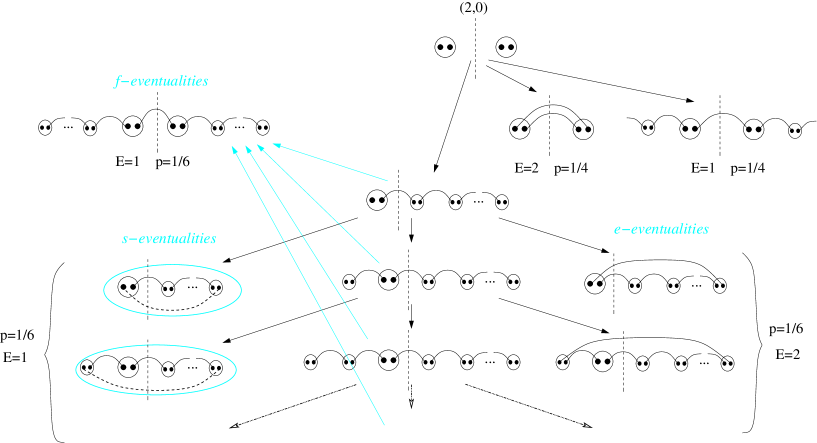
Figure 8: Reduced entanglement starting with a (2,0) partition bond. The various possibilities are illustrated on the same chart as Fig. 5. Note that we omit here the future reduced entanglement in the case of the resulting partition-spin-1.

V.4 Reduced entropy of a partition-bond of domain (1,1)

The entropy contribution and probabilities of a partition-bond of domain(1,1) are illustrated in Fig. 9. Note that the original singlet of the (1,1) domain does not contribute, since we considered it when it formed. The average contributions for this stage, together with the partition-spin-1 stage are:

$$E_{(1,1)}=\frac{1}{2}\cdot 1+\frac{1}{2}E_{1}=\frac{1}{2}+\frac{47}{2\cdot 40}$$ (94)

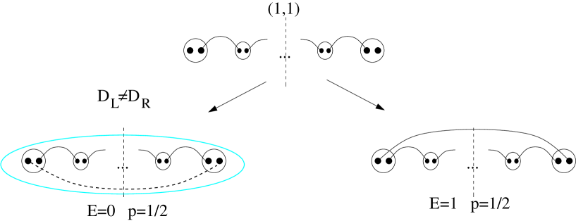
Figure 9: Reduced entanglement starting with a (1,1) partition bond. The various possibilities are illustrated on the same chart as Fig. 6. Note that we omit here the future reduced entanglement in the case of the resulting partition-spin-1.

V.5 Average total reduced entropy, and reduced central charge

The average total reduced entropy is:

$$\begin{array}[]{c}E_{total}=\frac{1}{3}E_{(1,1)}+\frac{2}{3}E_{(2,0)}\vspace{2mm}\\ =\frac{1}{6}+\frac{47}{6\cdot 40}+\frac{17}{3\cdot 6}+\frac{47}{9\cdot 40}\vspace{2mm}\\ =\frac{26}{18}-\frac{1}{8\cdot 18}\end{array}$$ (95)

We are now in a position to calculate the reduced central charge of the spin-1 critical point. The entanglement of a segment $L$ with the rest of the chain consists of:

$$\begin{array}[]{c}E=2\cdot\frac{E_{total}}{\ell_{total}}\ell_{L}\vspace{2mm}\\ =2\frac{\frac{26}{18}-\frac{1}{8\cdot 18}}{3/2}\ln L^{1/3}\vspace{2mm}\\ =\frac{1}{3}\frac{4}{3}\left(\frac{26}{18}-\frac{1}{8\cdot 18}\right)\ln L\vspace{2mm}\\ =\frac{1}{3}\left(2-\frac{1}{12}\right)\ln L\end{array}$$ (96)

Thus the reduced entropy central charge is:

$$c_{r}=\left(2-\frac{1}{12}\right)\ln 2\approx 1.917\ln 2$$ (97)

which should be compared to $c_{r}\approx 1.923\ln 2$ found numerically in the following section.

V.6 Numerical evaluation of the reduced entropy

The previous sections have described a method for tracking history dependence in the RSRG in order to extract the universal part of the entanglement entropy. Since this method is fairly intricate, a direct numerical check on the results is worthwhile. Although the full entanglement entropy cannot be calculated in closed form but only in a controlled approximation, the “reduced entropy” above can be calculated exactly. As a check, we now compute the reduced entropy by a numerical Monte Carlo simulation of the RSRG equations on a finite spin-1 chain.

For each subsystem size $N$, we average over 100 different intervals within each of 100 realizations. The initial distribution of Heisenberg couplings is tuned to lie at the critical point of an infinite chain. Fig. 10 shows the result: the reduced entropy of an interval of size $N$ is approximately

$$S(N)=1.9837+\left({1.923\ln 2\over 3}\right)\log_{2}N.$$ (98)

An overall statistical error in the numerical central charge of approximately $2\%$ is expected. The agreement of the numerical value $1.923\ln 2$ with the analytic result $(23/12)\ln 2$ can be taken to verify the history dependence obtained above. It appears that systematic errors in the numerics resulting from finite interval size and finite chain size ($10^{4}$ sites) are small. The remaining step is to use the same analysis of history dependence to obtain the true entanglement.

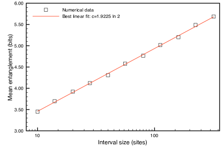
Figure 10: Numerical calculation of the reduced entropy $S_{\rm red}$ in the $s=1$ chain for intervals of various sizes $N$ within a chain of length $10^{4}$ sites. The fit is to $S_{\rm red}=S_{0}+(c/3)\log_{2}N$. The statistical standard deviation for each point shown is less than $5\%$.

VI Calculation of configurational entanglement in the spin-1 critical point

The last step on our way to the entanglement entropy of the spin-1 chain at its critical point is to understand the quantum entanglement of each closed singlet configuration. Many such configurations arise in the decimation process, but fortunately, for a high accuracy evaluation of the entanglement entropy, only few classes of these configurations are necessary. In this section we will discuss the entanglement in these configuration classes, both analytically and numerically.

VI.1 Simple configurations

Let us first consider the configurations arising from a (2,0) domain, Fig. 5. The simplest eventualities involve a decimation of the (2,0) domain while its two neighboring domains are identical. There are two possibilities. In eventuality $p_{-1}$ the neighboring domains are (0,2), and the decimation of the partition-bond involves forming a complete singlet between the spin-1 sites to the left and right of the partition:

$$\left|\psi_{\ell~{}r}\right\rangle=\frac{1}{2}\left(\hat{a}^{\dagger}_{\ell}\hat{b}^{\dagger}_{r}-\hat{b}^{\dagger}_{\ell}\hat{a}^{\dagger}_{r}\right)^{2}\left|0_{\ell~{}r}\right\rangle.$$ (99)

Since this is a Ma-Dasgupta decimation, the entanglement due to this step is independent of future steps. The entanglement between the left and the right sites is simply:

$$S_{p_{-1}}=\log_{2}3$$ (100)

since a trace of the left (or right) sites lead to an SO(3) symmetric density matrix for the right (left) site, and the spin-1 is completely undetermined, hence all three states contribute equally to the entropy.

The second possibility is that the (2,0) partition-bond is near (1,1) domains, which is a $p^{\prime}_{-1}$ eventuality. In this case, the domain walls surrounding the partition-bond are spin-1/2, and the decimation gives rise to one SBS, which gives:

$$S_{p^{\prime}_{-1}}=1.$$ (101)

A spin-1/2 degree of freedom is determined by the SBS on either side of the partition.

If the partition bond gets decimated while it is surrounded by two different domains, then the bond joins the (1,1) domain by the formation of an SBS. Since the (1,1) domain is assumed to be very large in the scaling limit, the domain walls on both its sides are uncorrelated. Nevertheless, we know that the partition is at a small finite distance to one of the (1,1) domain edges. In the next stages of the RG, the (1,1) domain expands, until it gets decimated in one of three ways. $f$ eventualities will result in the (1,1) domain of the bond joining another (1,1) domain through a Ma-Dasgupta decimation on its short side. This results in a closed cluster, with the entanglement entropy:

$$S_{f}=1.$$ (102)

A more difficult configuration occurs if the (1,1) domain containing the partition bond is decimated between two identical neighboring domains, while the partition bond is a distance $n$ from the edge of the (1,1) domain - $e_{n}$ eventuality of Fig. 5. In the absence of any ferromagnetic decimations, the entanglement of such a cluster can be calculated exactly, using the $SO(3)$ symmetry, and an important simplification. This simplification serves as a key ingredient of the numerical calculation of the entanglement entropy of more complicated configurations, that do involve ferromagnetic decimations. This is described in the next section.

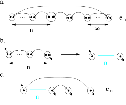
Figure 11: (a) A typical e-eventuality configuration. (b) Using the chain-rule singlet row reduction, we can reduce a chain of $n+1$ spin-1 sites with two dangling spin-1/2’s, to just two exact spin-1/2’s, which are related to the dangling edge spin-1/2’s as in Eq. (105). (c) Application of the chain-rule to the configuration in (a).

VI.2 Singlet-row reduction

To simplify the understanding of configurations such as in Fig. 11a, we will derive a rule that will replace the Schwinger-boson singlet chains which are completely contained in one side of the partition. Consider a chain of $n+1$ spin-1 sites, whose state consists of a singlet-row, i.e., a single connects sites $m$ and $m+1$ for all $m=0,\ldots,n-1$. Sites $0$ and $n$ have a dangling spin-1/2, thus there are four singlet-row states, which we write as:

$$\begin{array}[]{c}\left|\uparrow~{}(1,1)~{}\uparrow\right\rangle=\hat{a}^{\dagger}_{0}\hat{a}^{\dagger}_{n}\prod\limits_{i=0}^{n-1}\left(\hat{a}^{\dagger}_{i}\hat{b}^{\dagger}_{i+1}-\hat{b}^{\dagger}_{i}\hat{a}^{\dagger}_{i+1}\right)\left|0\right\rangle\vspace{2mm}\\ \left|\uparrow~{}(1,1)~{}\downarrow\right\rangle=\hat{a}^{\dagger}_{0}\hat{b}^{\dagger}_{n}\prod\limits_{i=0}^{n-1}\left(\hat{a}^{\dagger}_{i}\hat{b}^{\dagger}_{i+1}-\hat{b}^{\dagger}_{i}\hat{a}^{\dagger}_{i+1}\right)\left|0\right\rangle\vspace{2mm}\\ \left|\downarrow~{}(1,1)~{}\uparrow\right\rangle=\hat{b}^{\dagger}_{0}\hat{a}^{\dagger}_{n}\prod\limits_{i=0}^{n-1}\left(\hat{a}^{\dagger}_{i}\hat{b}^{\dagger}_{i+1}-\hat{b}^{\dagger}_{i}\hat{a}^{\dagger}_{i+1}\right)\left|0\right\rangle\vspace{2mm}\\ \left|\downarrow~{}(1,1)~{}\downarrow\right\rangle=\hat{b}^{\dagger}_{0}\hat{b}^{\dagger}_{n}\prod\limits_{i=0}^{n-1}\left(\hat{a}^{\dagger}_{i}\hat{b}^{\dagger}_{i+1}-\hat{b}^{\dagger}_{i}\hat{a}^{\dagger}_{i+1}\right)\left|0\right\rangle.\end{array}$$ (103)

The dangling spin-1/2’s at the edge are eventually locked into singlets, or ferromagnetic bonds which stretch past the partition. The sites $i=1,\,\ldots,\,n-1$ in the singlet row are inert, and do not contribute to entanglement, therefore calculation of the entanglement with them included is going to be quite difficult since they increase the Hilbert space involved by a factor of $3^{n-1}$. They do have an important role, however, which is to facilitate the correlations along the singlet chain.

But the correlations of the singlet-row can be taken into account while removing the interior inert sites. The correlations carried in the states in Eq. (103) are exhibited by the fact that the four states are not orthogonal. In particular:

$$\langle\uparrow~{}(1,1)~{}\downarrow\left|\downarrow~{}(1,1)~{}\uparrow\right\rangle=(-1)^{n}$$ (104)

This overlap is easily found, since it is the product of the amplitude of the state $m^{z}_{i}=0$ for all sites $0\leq i\leq n$. Note that the states in Eq. (103) are not normalized:

$$\begin{array}[]{c}\langle\uparrow~{}(1,1)~{}\uparrow\left|\uparrow~{}(1,1)~{}\uparrow\right\rangle=\langle\downarrow~{}(1,1)~{}\downarrow\left|\downarrow~{}(1,1)~{}\downarrow\right\rangle=N_{\uparrow\uparrow}\vspace{2mm}\\ \langle\uparrow~{}(1,1)~{}\downarrow\left|\uparrow~{}(1,1)~{}\downarrow\right\rangle=\langle\downarrow~{}(1,1)~{}\uparrow\left|\downarrow~{}(1,1)~{}\uparrow\right\rangle=N_{\uparrow\downarrow}\end{array}$$ (105)

Let us now define four new states that will be mutually orthogonal: $\left|\uparrow\uparrow\right\rangle,\,\left|\uparrow\downarrow\right\rangle,\left|\downarrow\uparrow\right\rangle,\,\left|\downarrow\downarrow\right\rangle$. We can capture the correlations in the singlet-row by writing:

$$\begin{array}[]{c}\left|\uparrow~{}(1,1)~{}\uparrow\right\rangle=\sqrt{N_{\uparrow\uparrow}}\left|\uparrow\uparrow\right\rangle\vspace{2mm}\\ \left|\downarrow~{}(1,1)~{}\downarrow\right\rangle=\sqrt{N_{\uparrow\uparrow}}\left|\downarrow\downarrow\right\rangle\vspace{2mm}\\ \left|\downarrow~{}(1,1)~{}\uparrow\right\rangle=a\left|\downarrow\uparrow\right\rangle+b\left|\uparrow\downarrow\right\rangle\vspace{2mm}\\ \left|\uparrow~{}(1,1)~{}\downarrow\right\rangle=a\left|\uparrow\downarrow\right\rangle+b\left|\downarrow\uparrow\right\rangle\end{array}$$ (106)

where $a$ and $b$ are real numbers which obey:

$$\begin{array}[]{c}a^{2}+b^{2}=N_{\uparrow\downarrow},\vspace{2mm}\\ 2ab=(-1)^{n},\end{array}$$ (107)

which is solved by:

$$\begin{array}[]{c}a=\frac{1}{2}\left(\sqrt{N_{\uparrow\downarrow}+(-1)^{n}}+\sqrt{N_{\uparrow\downarrow}-(-1)^{n}}\right),\vspace{2mm}\\ b=\frac{1}{2}\left(\sqrt{N_{\uparrow\downarrow}+(-1)^{n}}-\sqrt{N_{\uparrow\downarrow}-(-1)^{n}}\right).\end{array}$$ (108)

The norms $N_{\downarrow\downarrow},\,N_{\uparrow\downarrow}$ are found in App. A to be:

$$\begin{array}[]{c}N_{\uparrow\uparrow}=\frac{1}{2}\left(3^{n+1}+(-1)^{n}\right),\vspace{2mm}\\ N_{\uparrow\downarrow}=\frac{1}{2}\left(3^{n+1}-(-1)^{n}\right).\end{array}$$ (109)

The eigenvalues of the reduced density matrix of states that consist of singlet-rows written just using the dangling spins, as in Eq. (106), will be the same as those for the reduced density matrix involving all inert spin-1 sites, since the inner product of the states in Eq. (103) and (106) are the same. This presents an extreme simplification in terms of numerical evaluation of these eigenvalues.

VI.3 Entanglement of the level-0 (no FM clusters) e-eventualities and f-eventualities

Using the reduction of singlet-rows as in Eq. (106) we can reduce the configuration in Fig. 11a to that of Fig. 11c. The entanglement entropy of the $e_{n}$ eventuality is then easily calculated.

The first step is to write the state in Fig. 11a while ignoring the correlations along the singlet-row:

$$\begin{array}[]{c}\left|\psi\right\rangle=\left(\left|\uparrow_{1}\right\rangle\left|\downarrow_{4}\right\rangle-\left|\downarrow_{1}\right\rangle\left|\uparrow_{4}\right\rangle\right)\left(\left|\uparrow_{2}\right\rangle\left|\downarrow_{3}\right\rangle-\left|\downarrow_{2}\right\rangle\left|\uparrow_{3}\right\rangle\right)\vspace{2mm}\\ =\left|\uparrow_{1}\right\rangle\left|\downarrow_{4}\right\rangle\left|\uparrow_{2}\right\rangle\left|\downarrow_{3}\right\rangle-\left|\uparrow_{1}\right\rangle\left|\downarrow_{4}\right\rangle\left|\downarrow_{2}\right\rangle\left|\uparrow_{3}\right\rangle\vspace{2mm}\\ -\left|\downarrow_{1}\right\rangle\left|\uparrow_{4}\right\rangle\left|\uparrow_{2}\right\rangle\left|\downarrow_{3}\right\rangle+\left|\downarrow_{1}\right\rangle\left|\uparrow_{4}\right\rangle\left|\downarrow_{2}\right\rangle\left|\uparrow_{3}\right\rangle.\end{array}$$ (110)

Sites 1 and 2 are actually representatives of the dangling spin-1/2’s in the singlet-row, and therefore we apply to them the assignment of Eq. (106):

$$\begin{array}[]{c}\left|\psi\right\rangle\rightarrow\sqrt{N_{\uparrow\uparrow}}\left|\uparrow_{1}\right\rangle\left|\downarrow_{4}\right\rangle\left|\uparrow_{2}\right\rangle\left|\downarrow_{3}\right\rangle\vspace{2mm}\\ -a\left|\uparrow_{1}\right\rangle\left|\downarrow_{4}\right\rangle\left|\downarrow_{2}\right\rangle\left|\uparrow_{3}\right\rangle-b\left|\downarrow_{1}\right\rangle\left|\uparrow_{4}\right\rangle\left|\downarrow_{2}\right\rangle\left|\uparrow_{3}\right\rangle\vspace{2mm}\\ -a\left|\downarrow_{1}\right\rangle\left|\uparrow_{4}\right\rangle\left|\uparrow_{2}\right\rangle\left|\downarrow_{3}\right\rangle-b\left|\uparrow_{1}\right\rangle\left|\downarrow_{4}\right\rangle\left|\uparrow_{2}\right\rangle\left|\downarrow_{3}\right\rangle\vspace{2mm}\\ +\sqrt{N_{\uparrow\uparrow}}\left|\downarrow_{1}\right\rangle\left|\uparrow_{4}\right\rangle\left|\downarrow_{2}\right\rangle\left|\uparrow_{3}\right\rangle\end{array}$$ (111)

with $a$ and $b$ defined as in Eq. (108). The entanglement entropy follows from the eigenvalues of the reduced density matrix of the state $\left|\psi\right\rangle$ over sites 3 and 4. From SO(3) symmetry we can argue that the form of the reduced density matrix is:

$$\begin{array}[]{c}\hat{\rho}_{12}={\rm tr_{34}}\hat{\rho}=\vspace{2mm}\\ \frac{1}{3}\alpha\left(\left|\uparrow\uparrow\right\rangle\left\langle\uparrow\uparrow\right|+\left|\downarrow\downarrow\right\rangle\left\langle\downarrow\downarrow\right|+\frac{1}{2}\left|\uparrow\downarrow+\downarrow\uparrow\right\rangle\left\langle\uparrow\downarrow+\downarrow\uparrow\right|\right)\vspace{2mm}\\ +\beta\frac{1}{2}\left|\uparrow\downarrow-\downarrow\uparrow\right\rangle\left\langle\uparrow\downarrow-\downarrow\uparrow\right|\end{array}$$ (112)

where this representation breaks the reduced density matrix into the triplet and singlet sectors respectively, where it is already diagonal. We also have $\alpha=1-\beta$. To find $\alpha$ and $\beta$ all we need is to know the matrix element of one of the triplet states in $\hat{\rho}_{12}$. This is easily found:

$$\frac{1}{3}\alpha=\frac{N_{\uparrow\uparrow}}{2N_{\uparrow\uparrow}+2a^{2}+2b^{2}}=\frac{1}{2}\frac{N_{\uparrow\uparrow}}{N_{\uparrow\uparrow}+N_{\uparrow\downarrow}}$$ (113)

where the denominator is due to the normalization of the wave function in Eq. (111), and we used Eq. (107). This is then:

$$\alpha=\frac{3}{4}+\frac{(-1)^{n}}{4\cdot 3^{n}}$$ (114)

The entanglement entropy of this configuration is then:

$$S_{e_{n}}^{(0)}=-\alpha\log_{2}\frac{\alpha}{3}-(1-\alpha)\log_{2}(1-\alpha)=-\left(\frac{3}{4}+\frac{(-1)^{n}}{4\cdot 3^{n}}\right)\log_{2}\left(\frac{1}{4}+\frac{(-1)^{n}}{4\cdot 3^{n+1}}\right)-\left(\frac{1}{4}-\frac{(-1)^{n}}{4\cdot 3^{n}}\right)\log_{2}\left(\frac{1}{4}-\frac{(-1)^{n}}{4\cdot 3^{n}}\right)$$ (115)

The entanglement for the f-eventualities is remarkably simple, since in this case there is a spin-1/2 singlet crossing the partition, but this singlet is uncorrelated with the domain walls on the left and right of the partition bond. The configurational entanglement of an f-eventuality is:

$$S_{f_{n}}^{(0)}=1.$$ (116)

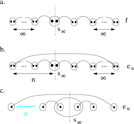
Figure 12: (a) A typical f-eventuality following a FM decimation. The entanglement entropy across the partition-site can be calculated exactly if we neglect correlations between the two spin-1/2 components of the partition site, a state which is denoted by $s_{\infty}$ (b) A typical e-eventuality configuration after a FM decimation. (c) Using the row-reduction rule we reduce the configuration from a to one of only six spin-1/2’s. Neglecting internal correlations in the partition site, we can calculate this entanglement entropy exactly.

VI.4 Entropy of level-1 eventualities neglecting history dependence of cluster

An approximate analytical answer for the entanglement can be obtained using the self-consistency method already at level-1, i.e., considering configurations with at most one FM decimations, by assuming that whenever a spin-1 cluster forms, its structure corresponds to $s_{\infty}$ of Figs. 4 and 5. This implies that the two spin-1/2’s participating in the ferromagnetic cluster are uncorrelated with the partition bond, and are infinitely removed from it. In this case the entropy contribution from level-n and level-n+1 become independent, and the entropy can be summed self-consistently, as described in Sec. VII.1.

For this purpose we need to derive the configurational entanglement of $e_{n}$ and f eventualities of spin-1 sites, as in Fig. 4, assuming the initial FM spin-1 cluster consists of two uncorrelated spin-1/2 sites. Let us begin with the simpler f-eventuality. This case is depicted in Fig. 12a. The entanglement of this configuration, with the spin-1 partition-site containing two spin-1/2’s which are uncorrelated before they form the FM cluster, is easily computed to be:

$$S_{f}^{(1)}=2-\frac{1}{2}\log_{2}3.$$ (117)

Next we find the entanglement of the $e_{n}$ eventualities of this setup, depicted in Fig. 12b. This setup is simplified to a six-site configuration, with the partition situated in the middle (Fig. 12c). Once the three spins to the right of the partition are traced out, we are left with a 3-spin-1/2 density matrix, which for brevity we do not quote here, of a complicated mixed state. Due to rotational SO(3) symmetry, however, this density matrix breaks down to invariant sectors corresponding to the decomposition:

$$1/2\times 1/2\times 1/2=3/2+1/2+1/2.$$ (118)

One sector is the spin-3/2 subspace, and two other invariant subspaces will correspond to the total spin of the three sites being 1/2. Furthermore the restriction of the reduced density matrix on each of the invariant subspaces, should be of diagonal form. In the basis $\left|3/2,m\right\rangle(m=3/2,\ldots,-3/2),\,\left|1/2,m\right\rangle(m=1/2,-1/2),\,\left|1/2^{\prime},m\right\rangle(m=1/2,-1/2)$ the reduced density matrix is:

$$\hat{\rho}_{1,2,3}={\rm diag}\{\alpha_{n},\,\alpha_{n},\,\alpha_{n},\,\alpha_{n},\,\beta_{n},\,\beta_{n},\,\gamma_{n},\,\gamma_{n}\}$$ (119)

Finding $\alpha,\,\beta$, and $\gamma$ can be done analytically. $\alpha$ is the easiest to obtain, since we know from rotational symmetry that the state $\left|\uparrow_{1}\uparrow_{2}\uparrow_{3}\right\rangle$ is an eigenstate. We readily obtain:

$$\alpha_{n}=\frac{1}{24}\left(1-(-1/3)^{n}\right)$$ (120)

Obtaining $\beta_{n}$ is more involved, but can be done by looking at the restriction of the reduced density matrix to the invariant subspace of $m_{z}=1/2$ ($\left|\downarrow_{1}\uparrow_{2}\uparrow_{2}\right\rangle,\,\left|\uparrow_{1}\downarrow_{2}\uparrow_{3}\right\rangle,\,\left|\uparrow_{1}\uparrow_{2}\downarrow_{3}\right\rangle$), and removing from it the subspace of $\left|3/2,m_{z}=1/2\right\rangle=\frac{1}{\sqrt{3}}\left(\left|\downarrow_{1}\uparrow_{2}\uparrow_{2}\right\rangle+\left|\uparrow_{1}\downarrow_{2}\uparrow_{3}\right\rangle+\left|\uparrow_{1}\uparrow_{2}\downarrow_{3}\right\rangle\right)$. This leaves us with an easily diagnosable $2\times 2$ matrix with eigenvalues:

$$\begin{array}[]{c}\beta_{n}=\frac{1}{24}\left(5+(-1/3)^{n}+\sqrt{\left(4+2\cdot(-1/3)^{n}\right)^{2}-24\cdot(-1/3)^{n}+24/3^{2n}}\right)\vspace{2mm}\\ \gamma_{n}=\frac{1}{24}\left(5+(-1/3)^{n}-\sqrt{\left(4+2\cdot(-1/3)^{n}\right)^{2}-24\cdot(-1/3)^{n}+24/3^{2n}}\right)\end{array}$$ (121)

The above formulas, Eqs. (120) and (121) obtain for $n>1$. The cases of $n=-1$, $n=0$, and $n=1$ need to be calculated separately, but their contribution to the entanglement entropy is very simple. The cases of $e_{-1}$ and $e_{0}$ implies the spin-1 partition site is decimated via two singlets that link it to two uncorrelated spin-1/2’s to one of its sides. Upon tracing out of that side of the partition, we obtain a reduced matrix that describes a spin-1/2 with equal probability of pointing up or down, hence, $e_{0}^{(1)}=e_{-1}^{(1)}=1$.

An analysis of the $e_{1}$ case can proceed along similar lines to the one above and to the analysis of the $e_{n}$ eventualities as in Eq. (114), to obtain:

$$e_{0}^{(1)}=4\cdot\frac{1}{18}\log_{2}18+2\cdot\frac{7}{18}\log_{2}\frac{18}{7}$$ (122)

Thus the entanglement of an $e_{n}$ cluster containing a spin-1 partition-site is:

$$S_{e_{n}}^{(1)}=\left\{\begin{array}[]{cr}1&n=-1,1\vspace{2mm}\\ 4\cdot\frac{1}{18}\log_{2}18+2\cdot\frac{7}{18}\log_{2}\frac{18}{7}&n=1\vspace{2mm}\\ -4\alpha_{n}\log_{2}\alpha_{n}-2\beta_{n}\log_{2}\beta_{n}-2\gamma_{n}\log_{2}\gamma_{n}&n>1.\end{array}\right.$$ (123)

VII Entanglement entropy of the spin-1 chain

We are now at a position to combine the above results into the entanglement entropy, as given in Eqs. (29) and (30), to obtain:

$$c_{eff}=\frac{2\overline{S}_{total}}{\overline{\ell}}\ln 2.$$ (124)

In Sec. IV we found that:

$$\overline{\ell}=\frac{3}{2}.$$ (125)

In the remains of this section, we will extract the value of

$$\overline{S}_{total}=\sum\limits_{c}p_{c}S_{c},$$ (126)

where $p_{c}$ is the probability for a configuration $c$ to occur, and $S_{c}$ is the entanglement entropy associated with it.

One major obstacle is presented by the ferromagnetic decimations, which give rise to complex quantum states. A decimated configuration can involve any number, $n$, of spin-1 ferromagnetic decimation steps, but with a rapidly decaying probability of $1/6^{n}$ (see Eq. 56). The configurational entropy $\overline{S}_{total}$ can be obtained to arbitrary accuracy by calculating exactly the configurational-entropy of all configurations with $n-1$ ferromagnetic decimations, and applying the approximation that the $n$-th level Ferromagnetic decimation is between two spin-1/2’s that are infinitely far from the partition, and thus correspond to the $s_{\infty}$ eventuality. This provides a result for $\overline{S}_{total}$ which has accuracy of:

$$\Delta S_{total}\approx\frac{1}{6\cdot 6^{n}}.$$ (127)

In what follows we obtain the computer-free $n=1$ result, and using Mathematica to calculate and sum the configurational entropy, we go up to level $n=3$, with accuracy of $\sim 10^{-3}$.

VII.1 Entanglement entropy from level 0 and 1

The entropy of the configurations computed exactly in Sec. VI.3 and VI.4 can be summed up to give the $n=1$ approximation for $\overline{S}_{total}$. In this approximation we have:

$$\overline{S}_{total}=\frac{2}{3}\overline{S}_{(2,0)}+\frac{1}{3}\overline{S}_{(1,1)},$$ (128)

where $\overline{S}_{(2,0)}$ and $\overline{S}_{(1,1)}$ are the average entanglement entropies across partition-bonds that are initially (2,0) and (1,1) domains respectively.

Let us first find the average entanglement with the partition bond being a (2,0) domain initially. Looking at Fig. 5 we have:

$$\overline{S}_{(2,0)}=\overline{S}_{(2,0)~{}e}^{(0)}+\overline{S}_{(2,0)~{}f}^{(0)}+\overline{S}_{(2,0)~{}s}^{(0)},$$ (129)

where $S_{c}^{(0)}$ is the average entanglement entropy due to configuration $c$ with $c=e,\,f,\,s$. The entanglement due to the level-0 e-eventualities starting with a (2,0) or (0,2) domain is given by:

$$\overline{S}_{(2,0)~{}e}^{(0)}=p_{p^{\prime}_{-1}}\cdot 1+p_{p^{\prime}_{-1}}\cdot\log_{2}3+\sum\limits_{n=0}^{\infty}S_{e_{n}}^{(0)}\cdot\frac{1}{8\cdot 4^{n}},$$ (130)

where $p_{p^{\prime}_{-1}}=p_{p_{-1}}=1/4$.

The entanglement due to level-0 f-entanglement starting with a (2,0) domain is:

$$\overline{S}_{(2,0)~{}f}^{(0)}=\sum\limits_{n=0}^{\infty}S_{f_{n}}^{(0)}\cdot\frac{1}{8\cdot 4^{n}}=\frac{1}{6}.$$ (131)

To complete the calculation we need to add to these the entanglement of the spin-1 cluster that forms due to the s-eventualities, $\overline{S}_{(2,0)~{}s}^{(0)}$. In this section we approximate the spin-1 cluster as consisting of uncorrelated spins. This produces average configurational entropy we denote as $\overline{S}_{s}^{\infty}$, and thus:

$$\overline{S}_{(2,0)~{}s}^{(0)}\approx p_{s}(1+\overline{S}_{s}^{\infty})=\frac{1}{6}(1+\overline{S}_{s}^{\infty}),$$ (132)

where the one in the brackets is due to the SBS formed on the partition-bond in the process.

The equivalent contributions to level-0 when the partition-bond is a (1,1) domain initially is quite simple. With probability $1/2$ the partition bond undergoes a Ma-Dasgupta decimation which has configurational entropy 1, which implies:

$$\overline{S}_{(1,1)~{}e}^{(0)}=1/2\cdot 1=1/2.$$ (133)

The remaining probability is that the partition-bond is decimated ferromagnetically. Thus:

$$\overline{S}_{(1,1)}=\overline{S}_{(1,1)~{}e}+\overline{S}_{(1,1)~{}s}^{(0)}\approx\frac{1}{2}+\frac{1}{2}\overline{S}_{s}^{\infty}.$$ (134)

We now calculate $\overline{S}_{s}^{\infty}$. Looking at Fig. 4, we see that:

$$\overline{S}_{s}^{\infty}=\overline{S}_{e}^{(1)}+\overline{S}_{f}^{(1)}+\overline{S}_{s}^{(1)}.$$ (135)

The entanglement of an $e_{n}$ cluster containing a spin-1 partition-site is:

$$\overline{S}_{e~{}\infty}^{(1)}=\frac{5}{8}\cdot 1+\frac{1}{32}e_{0}^{(1)}+\sum\limits_{n=2}^{\infty}\frac{1}{8\cdot 4^{n}}\left(-4\alpha_{n}\log_{2}\alpha_{n}-2\beta_{n}\log_{2}\beta_{n}-2\gamma_{n}\log_{2}\gamma_{n}\right).$$ (136)

where we make use of the configurational entanglement we find in Sec. VI.4, and where the $\alpha_{n},\,\beta_{n},\,\gamma_{n}$ are defined in Eqs. (120) and (121).

$\overline{S}_{f}^{(1)}$ is much simpler, and from Eq. (117), which gives the configurational entropy, we get:

$$\overline{S}_{f~{}\infty}^{(1)}=\frac{1}{6}(2-\log_{2}3).$$ (137)

After considering all e- and f- eventualities, only one more possibility remains, which is the formation of a new spin-1 cluster via a ferromagnetic decimation. If we once more pursue the approximation of assuming that the spin-1 partition-site forms out of two spin-1/2’s that are infinitely far from the partition, then we can self consistently connect the entanglement of this eventuality with the one calculated in this section. Thus we write:

$$\overline{S}_{s}^{\infty}=\overline{S}_{f~{}\infty}^{(1)}+\overline{S}_{e~{}\infty}^{(1)}+\frac{1}{6}\overline{S}_{s}^{\infty}.$$ (138)

Isolating $\overline{S}_{s}^{\infty}$, and plugging in all numbers from Eqs. (117) - (136) we obtain the approximate cluster entropy due to a spin-1 partition site:

$$\overline{S}_{s}^{\infty}=1.33495.$$ (139)

Note that this is an overestimate since we neglect correlations within the spin-1 effective site. These correlations reduce the entanglement entropy.

Combining the results above, and substituting into Eq. (128) we obtain that the average configurational entanglement is:

$$\overline{S}_{total}=\frac{1}{3}\cdot 1.16748+\frac{2}{3}\cdot 1.48271=1.3776.$$ (140)

VII.2 Entanglement entropy from level 3 self consistent approximation

In principle, we could obtain an exact result for the configurational entanglement by summing up the entanglement of each configuration times its probabilities. The probabilities of each and every configuration are well known, but at levels higher than one FM decimation, we can only obtain the configurational entropy using a computer. Nevertheless, this part of the calculation can be automated.

The exact solution can be expressed using the following pattern. We can encode the eventualities of decimated configurations as:

$$\pi_{0}\circ\pi_{1}\circ\pi_{2}\circ\ldots\circ\pi_{p},$$ (141)

where the $\pi_{i}$ describe what happens to the cluster at each level of FM decimation. A series can terminate at $\pi_{0}=p_{-1},\,p^{\prime}_{-1},\,e_{n}^{R/L},\,f_{n}^{R/L}$, or begin by forming a FM spin-1 partition site with $\pi_{0}=s_{n}^{R/L}$. The following p-1 steps can also be any sequence of FM spin-1 site formation, $\pi_{i}=s_{n_{i}}^{R/L}$. The last step, $\pi_{p}$, can be any of $\pi_{p}=e_{n_{p}}^{R/L},\,f_{n_{p}}^{R/L}$, which renders the cluster decimated. Note that at levels $p>0$, $e_{n_{p}}$ has $n_{p}=-1,\,0,\,1,\ldots$.

Hence, an exact calculation can be written as:

$$\overline{S}_{total}=\sum\limits_{p=0}^{\infty}\sum\limits_{\{\pi_{i}|i=0,\,\ldots,\,p\}}\left(\prod\limits_{i=0}^{p}P_{\pi_{i}}\right)S_{\left(\pi_{0}\circ\pi_{1}\circ\pi_{2}\circ\ldots\circ\pi_{p}\right)}.$$ (142)

We know the probability of each eventuality exactly, as explained in Sec. (IV). The remaining part is the configurational entropy. As explained above, we can calculate this entropy analytically for simple configurations. But to obtain a conclusive answer, we carry out a higher level calculation using the computer program Mathematica. Using the reduction trick of Sec. VI.2, we can simplify any configuration of level-n to a density matrix involving at most $4+3n$ spins. This allows an exact numerical computation.

We carried out this computation up to level-3 configurations. The result for the average configurational entropy was:

$$\overline{S}_{total}=1.3327-0.001.$$ (143)

Note that this answer is an overestimate (hence the subtraction sign for error indication), and thus can not be taken to be exactly 4/3. The closeness of the answer to 4/3, however, is quite mysterious.

VII.3 Effective central charge results

The effective central charge of the critical spin-1 chain is thus:

$$c_{eff}^{(r_{c})}=\frac{4}{3}\cdot 1.3327\cdot\ln 2=1.232$$ (144)

and the entanglement entropy between a segment of length L and the rest of the chain is:

$$\frac{1}{3}1.232\log_{2}L.$$ (145)

where we use the level-3 result above. Note that $c_{eff}^{(r_{c})}=16/9-\epsilon$ where $\epsilon\approx 10^{-4}$. In the next section we discuss the significance of our results in the context of infinite-randomness fixed points.

VIII Discussion

Several random quantum critical points in 1D are now known to have logarithmic divergences of entanglement entropy with universal coefficients, as in the pure case. So far, all analyzed systems were infinite randomness critical points in the Random-singlet universality class. Refael and Moore (2004); Santachiara (2006); Laflorencie (2005); Bonesteel and Yang (2006) Summarizing the results for these systems is possible with the formula:

$$S\sim\frac{1}{3}\ln D\log_{2}L,$$ (146)

where $D$ is the dimension of the gapless sector of the Hilbert-space on each site, which generalizes to the quantum dimension in the case of the golden-chain. Bonesteel and Yang (2006) Hence the ’effective central charge’ for these critical points is simply:

$$c_{eff}=\ln D.$$ (147)

The present work investigates the disorder-averaged entanglement entropy of a different universality class within the infinite-randomness framework: the spin-1 Haldane-RS critical point. We indeed find a different result than Eq. (147), which arises from a more complex structure of the spin-1 Haldane-RS point. We find the entanglement entropy for this fixed point to be:

$$S\sim\frac{1}{3}{c_{eff}}\log_{2}L=\frac{1}{3}\frac{4}{3}\cdot 1.3327\cdot\ln 2\log_{2}L.$$ (148)

Our calculation required both the exact probabilistic description of the low-energy structure given by RSRG, and the individual determination of the quantum entanglement of each spin configuration in the low-energy structure.

An open question is whether other physical properties are related to the universal coefficient. In pure 1D quantum critical systems described by 2D classical theories with conformal invariance, the central charge $c$ controls several important physical properties beyond the entanglement entropy. An example is the specific heat at low temperatures: because the central charge determines the change in free energy when the 2D classical system is compactified in one direction (i.e., put on a cylinder), the quantum system at finite temperature has a contribution to the specific heat that is proportional to $c$.

The central charge also gives some information about the renormalization-group flows connecting different critical points because of Zamolodchikov’s $c$-theorem: Zamolodchikov (1986) RG flows are from high central charge to low central charge, compatible with the heuristic view of the RG as “integrating out” degrees of freedom. Ref. Castro Neto and Fradkin, 1993 goes as far as defining a c-function for a finite-temperature quantum system, which decreases with decreasing temperatures, as it flows to a stable conformally-invariant fixed point. It is logical to ask Vidal et al. (2003); Refael and Moore (2004) whether entanglement entropy can similarly be used to predict the direction of real-space RG flows. As pointed out in the introduction, Sec. I, this question separates in two:

1. flows from pure conformally-invariant points to infinite randomness points,

2. flow between two different infinite-randomness fixed points.

Recently, a counterexample for question (1) was found by Santachiara:Santachiara (2006) for the random quantum parafermionic Potts model with $N>41$, the random critical point was found to have larger entanglement than the pure critical point, even though randomness is relevant at the pure critical point. This point too obeys Eq. (147) with $D\rightarrow N$. Until now, there were no models in which we could ask the second question; the spin-1 random Heisenberg model provides the first test of case (2).

The critical point of the spin-1 Heisenberg model we found the effective central charge

$$c^{(r_{c})}_{eff}=1.232\approx\frac{16}{9}\ln 2.$$ (149)

As shown in Fig. 1, this point is unstable towards the spin-1 RS point with entanglement entropy:

$$c^{RS}_{eff}=\ln 3=1.099<c^{(r_{c})}_{eff}.$$ (150)

On the weak randomness side, the critical point is unstable towards the Haldane phase (with topological order, but with a suppressed gap due to Griffiths effects. Damle (2002); Motrunich et al. (2001) The Haldane phase does not have a $\ln L$ term at all. Hence, within the critical points of the random Heisenberg model, effective $c$ does decrease along flows, which agrees with case 2 above.

The Haldane-RS critical point of the random spin-1 chain is thought to be the terminus of a flow beginning with the pure spin-1 chain in Eq. (4), which is a $k=2$ WZW theory with central charge $c=3/2$. Since $c^{(r_{c})}_{eff}=1.232<3/2$, the effective Central charge indeed also decreases along the flow line from the pure to the random critical fixed point, as posited in case 1 above.

In order to make clear the similarity between the random-singlet phase of the spin-1 chain and the random-singlet phase of the spin-1/2 chain, it seems worthwhile to introduce a modified central charge that is the coefficient of the $1/3\log_{2}L$ divided by the measure of the local ungapped Hilbert space in each site, $\ln D$. This clearly puts all random singlet phases on the same footing even when arising in different microscopic systems. In addition, one may ask whether such a redefined measure may always reduce along RG flows, even those connecting pure fixed points to random ones.

An interesting difference between the spin-1 case we study and previous work, is that for RS phases the exact logarithmic divergence of entanglement entropy can be found in closed form using the RG history approach, while for spin-1, the true entanglement entropy seems to depend on the entanglement values of an infinite number of nonequivalent, irreducible sub-chains. This turn of events motivated us to define the ’reduced entropy’ in Sec. V. This simplified measure of the entanglement counts directly how many SBS’s connect the segment $L$ with the rest of the chain, and neglects the correlation induced by the SBS’s. Our analysis allowed an exact calculation of the reduced entanglement, which yielded:

$$c^{reduced}_{eff}=\frac{23}{12}\ln 2\approx 1.329.$$ (151)

A numerical test using a computerized application of the RSRG confirmed this exact analytical result (see Sec. V.6), thus affirming the history-dependence segment of our approach.

In light of the simplicity of the definition of the reduced entanglement, it is interesting to ask how is relates to the real quantum entanglement. Since it neglects correlations between singlets, the reduced entanglement is most likely an overestimate of the quantum entanglement. This remains to be proved generally. In the spin-1/2 case, the reduced entanglement and the real entanglement coincide. For the spin-1 RS-Haldane critical point, we have:

$$c^{reduced}_{eff}\approx 1.329>1.232\approx c^{(r_{c})}_{eff}$$ (152)

Hence the reduced entropy is bigger by about 10$\%$. If there were some simplifying relation in the entanglement of these irreducible units, as there is for the reduced entanglement, then our method would give a closed form, but barring that it seems that entanglement entropy is a less natural object in the real-space renormalization group for higher spin than the (unphysical) reduced entropy.

Future directions include, needless to say, the calculation of the universal entanglement entropy in other infinite-randomness non RS fixed points. Our method can be straightforwardly applied to $s>1$ chains. But an exciting possibility is the consideration of the infinite-randomness fixed points arising in non-abelian spin chains.Bonesteel et al. The random-singlet subset of this class of fixed points were recently studied in Ref. Bonesteel and Yang, 2006.

Appendix A Calculation of $N_{\downarrow\downarrow},\,N_{\uparrow\downarrow}$

In Sec. VI.2 we defined the states:

$$\begin{array}[]{c}\left|\uparrow~{}(1,1)~{}\uparrow\right\rangle=\hat{a}^{\dagger}_{0}\hat{a}^{\dagger}_{n}\prod\limits_{i=0}^{n-1}\left(\hat{a}^{\dagger}_{i}\hat{b}^{\dagger}_{i+1}-\hat{b}^{\dagger}_{i}\hat{a}^{\dagger}_{i+1}\right)\left|0\right\rangle\vspace{2mm}\\ \left|\uparrow~{}(1,1)~{}\downarrow\right\rangle=\hat{a}^{\dagger}_{0}\hat{b}^{\dagger}_{n}\prod\limits_{i=0}^{n-1}\left(\hat{a}^{\dagger}_{i}\hat{b}^{\dagger}_{i+1}-\hat{b}^{\dagger}_{i}\hat{a}^{\dagger}_{i+1}\right)\left|0\right\rangle\vspace{2mm}\\ \left|\downarrow~{}(1,1)~{}\uparrow\right\rangle=\hat{b}^{\dagger}_{0}\hat{a}^{\dagger}_{n}\prod\limits_{i=0}^{n-1}\left(\hat{a}^{\dagger}_{i}\hat{b}^{\dagger}_{i+1}-\hat{b}^{\dagger}_{i}\hat{a}^{\dagger}_{i+1}\right)\left|0\right\rangle\vspace{2mm}\\ \left|\downarrow~{}(1,1)~{}\downarrow\right\rangle=\hat{b}^{\dagger}_{0}\hat{b}^{\dagger}_{n}\prod\limits_{i=0}^{n-1}\left(\hat{a}^{\dagger}_{i}\hat{b}^{\dagger}_{i+1}-\hat{b}^{\dagger}_{i}\hat{a}^{\dagger}_{i+1}\right)\left|0\right\rangle.\end{array}$$ (153)

We found that these states do not constitute a orthogonal set since:

$$\langle\uparrow~{}(1,1)~{}\downarrow\left|\downarrow~{}(1,1)~{}\uparrow\right\rangle=(-1)^{n}.$$ (154)

To be able to carry out the procedure outlined in Sec. VI.2 we need to calculate the norms of these states, which will than allow a transformation into an orthonormal combination.

From standard transfer matrix techniques, and Wick contractions, we find for $N_{\uparrow\uparrow}$:

$$\begin{array}[]{c}N_{\uparrow\uparrow}=\left\langle 0\right|\left(\hat{a}_{0}\hat{a}_{n}\prod\limits_{i=0}^{n-1}\left(\hat{a}_{i}\hat{b}_{i+1}-\hat{b}_{i}\hat{a}_{i+1}\right)\right)\hat{a}^{\dagger}_{0}\hat{a}^{\dagger}_{n}\prod\limits_{i=0}^{n-1}\left(\hat{a}^{\dagger}_{i}\hat{b}^{\dagger}_{i+1}-\hat{b}^{\dagger}_{i}\hat{a}^{\dagger}_{i+1}\right)\left|0\right\rangle\vspace{2mm}\\ =\left(\begin{array}[]{c}2\vspace{2mm}\\ 1\end{array}\right)^{T}\left(\begin{array}[]{cc}1&2\vspace{2mm}\\ 2&1\end{array}\right)^{n-1}\left(\begin{array}[]{c}1\vspace{2mm}\\ 2\end{array}\right)\vspace{2mm}\\ =\left(\begin{array}[]{c}2\vspace{2mm}\\ 1\end{array}\right)^{T}\frac{1}{\sqrt{2}}\left(\begin{array}[]{cc}1&1\vspace{2mm}\\ 1&-1\end{array}\right)\left(\begin{array}[]{cc}3&0\vspace{2mm}\\ 0&-1\end{array}\right)^{n-1}\frac{1}{\sqrt{2}}\left(\begin{array}[]{cc}1&1\vspace{2mm}\\ 1&-1\end{array}\right)\left(\begin{array}[]{c}1\vspace{2mm}\\ 2\end{array}\right)\vspace{2mm}\\ =\frac{1}{2}\left(\begin{array}[]{c}3\vspace{2mm}\\ 1\end{array}\right)^{T}\left(\begin{array}[]{cc}3&0\vspace{2mm}\\ 0&-1\end{array}\right)^{n-1}\left(\begin{array}[]{c}3\vspace{2mm}\\ -1\end{array}\right)=\frac{1}{2}\left(3^{n+1}+(-1)^{n}\right).\end{array}$$ (155)

Very similarly, for $N_{\uparrow\downarrow}$:

$$\begin{array}[]{c}N_{\uparrow\downarrow}=\left\langle 0\right|\left(\hat{a}_{0}\hat{b}_{n}\prod\limits_{i=0}^{n-1}\left(\hat{a}_{i}\hat{b}_{i+1}-\hat{b}_{i}\hat{a}_{i+1}\right)\right)\hat{a}^{\dagger}_{0}\hat{b}^{\dagger}_{n}\prod\limits_{i=0}^{n-1}\left(\hat{a}^{\dagger}_{i}\hat{b}^{\dagger}_{i+1}-\hat{b}^{\dagger}_{i}\hat{a}^{\dagger}_{i+1}\right)\left|0\right\rangle\vspace{2mm}\\ =\left(\begin{array}[]{c}2\vspace{2mm}\\ 1\end{array}\right)^{T}\left(\begin{array}[]{cc}1&2\vspace{2mm}\\ 2&1\end{array}\right)^{n-1}\left(\begin{array}[]{c}2\vspace{2mm}\\ 1\end{array}\right)\vspace{2mm}\\ =\left(\begin{array}[]{c}2\vspace{2mm}\\ 1\end{array}\right)^{T}\frac{1}{\sqrt{2}}\left(\begin{array}[]{cc}1&1\vspace{2mm}\\ 1&-1\end{array}\right)\left(\begin{array}[]{cc}3&0\vspace{2mm}\\ 0&-1\end{array}\right)^{n-1}\frac{1}{\sqrt{2}}\left(\begin{array}[]{cc}1&1\vspace{2mm}\\ 1&-1\end{array}\right)\left(\begin{array}[]{c}2\vspace{2mm}\\ 1\end{array}\right)\vspace{2mm}\\ =\frac{1}{2}\left(\begin{array}[]{c}3\vspace{2mm}\\ 1\end{array}\right)^{T}\left(\begin{array}[]{cc}3&0\vspace{2mm}\\ 0&-1\end{array}\right)^{n-1}\left(\begin{array}[]{c}3\vspace{2mm}\\ 1\end{array}\right)=\frac{1}{2}\left(3^{n+1}-(-1)^{n}\right).\end{array}$$ (156)

References

- Sachdev (1999) S. Sachdev, Quantum phase transitions (Cambridge University Press, London, 1999).
- Holzhey et al. (1994) C. Holzhey, F. Larsen, and F. Wilczek, Nucl. Phys. B 424, 44 (1994).
- Vidal et al. (2003) G. Vidal, J. I. Latorre, E. Rico, and A. Kitaev, Phys. Rev. Lett. 90, 227902 (2003).
- Calabrese and Cardy (2004) P. Calabrese and J. Cardy, J. Stat. Mech. 06, P06002 (2004).
- Ryu and Takayanagi (2006a) S. Ryu and T. Takayanagi, Phys. Rev. Lett. 96, 181602 (2006a).
- Srednicki (1993) M. Srednicki, Phys. Rev. Lett. 71, 666 (1993).
- Gioev and Klich (2006) D. Gioev and I. Klich, Phys. Rev. Lett. 96, 100503 (2006).
- Wolf (2006) M. M. Wolf, Phys. Rev. Lett. 96, 010404 (2006).
- Ryu and Takayanagi (2006b) S. Ryu and T. Takayanagi, JHEP 0608, 045 (2006b).
- Fradkin and Moore (2006) E. Fradkin and J. E. Moore, Phys. Rev. Lett. 97, 050404 (2006).
- Zamolodchikov (1986) A. B. Zamolodchikov, JETP Lett. 43, 730 (1986).
- Igloi and Monthus (2005) F. Igloi and C. Monthus, Phys. Rep. 412, 277 (2005).
- Fisher (1994) D. S. Fisher, Phys. Rev. B 50, 3799 (1994).
- Refael and Moore (2004) G. Refael and J. E. Moore, Phys. Rev. Lett. 93, 260602 (2004).
- Laflorencie (2005) N. Laflorencie, Phys. Rev. B 72, 140408 (2005).
- De Chiara et al. (2006) G. De Chiara, S. Montangero, P. Calabrese, and R. Fazio, J. of Stat. Mech. 0603, 001 (2006).
- Fisher (1995) D. S. Fisher, Phys. Rev. B 51, 6411 (1995).
- Santachiara (2006) R. Santachiara, J.Stat. Mech. p. L06002 (2006).
- Bonesteel and Yang (2006) N. E. Bonesteel and K. Yang, Infinite randomness fixed points for chains of non-abelian quasiparticles, cond-mat/0612503 (2006).
- Igloi et al. (2007) F. Igloi, R. Juhasz, and Z. Zimboras, Entanglement entropy of aperiodic quantum spin chains, cond-mat/0701527 (2007).
- Hyman and Yang (1997) R. A. Hyman and K. Yang, Phys. Rev. Lett. 78, 1783 (1997).
- Monthus et al. (1998) C. Monthus, O. Golinnelli, and T. Jolicoeur, Phys. Rev. B 58, 805 (1998).
- Lin et al. (2003) Y. C. Lin, R. Melin, H. Rieger, and F. Igloi, Physical Review B 68, 024424 (2003).
- Boechat et al. (1996) B. Boechat, A. Saguia, and M. Continentino, Solid State Communications 98, 411 (1996).
- Saguia et al. (2002) A. Saguia, B. Boechat, and M. A. Continentino, Phys. Rev. Lett. 89, 117202 (2002).
- Refael et al. (2002) G. Refael, S. Kehrein, and D. S. Fisher, Phys. Rev. B 66, 060402 (2002).
- Damle and Huse (2002) K. Damle and D. A. Huse, Phys. Rev. Lett. 89, 277203 (2002).
- Takhtajan (1982) L. Takhtajan, Phys. Lett. A 87, 479 (1982).
- Babudjian (1982) J. Babudjian, Phys. Lett. A 90, 479 (1982).
- Affleck (1986) I. Affleck, Phys. Rev. Lett. 56, 746 (1986).
- Ma et al. (1979) S. K. Ma, C. Dasgupta, and C. K. Hu, Phys. Rev. Lett. 43, 1434 (1979).
- Dasgupta and Ma (1980) C. Dasgupta and S. K. Ma, Phys. Rev. B 22, 1305 (1980).
- Fisher et al. (1999) D. S. Fisher, P. L. Doussal, and C. Monthus, Phys. Rev. E 59, 4795 (1999).
- Haldane (1983) F. D. M. Haldane, Phys. Rev. Lett. 50, 1153 (1983).
- Affleck et al. (1987) I. Affleck, T. Kennedy, E. H. Lieb, and H. Tasaki, Phys. Rev. Lett. 59, 799 (1987).
- Motrunich et al. (2001) O. Motrunich, K. Damle, and D. A. Huse, Phys. Rev. B 63, 224204 (2001).
- Damle (2002) K. Damle, Phys. Rev. B 66, 104425 (2002).
- Castro Neto and Fradkin (1993) A. H. Castro Neto and E. Fradkin, Nuc. Phys. B 400, 525 (1993).
- (39) N. Bonesteel, J. Moore, G. Refael, and K. Yang, In preparation.