Switchable coupling between charge and flux qubits

Xiao-Ling He Department of Physics and Surface Physics Laboratory (National Key Laboratory), Fudan University, Shanghai 200433, China Frontier Research System, The Institute of Physical and Chemical Research (RIKEN), Wako-shi 351-0198, Japan    J. Q. You Department of Physics and Surface Physics Laboratory (National Key Laboratory), Fudan University, Shanghai 200433, China Frontier Research System, The Institute of Physical and Chemical Research (RIKEN), Wako-shi 351-0198, Japan    Yu-xi Liu Frontier Research System, The Institute of Physical and Chemical Research (RIKEN), Wako-shi 351-0198, Japan    L. F. Wei Frontier Research System, The Institute of Physical and Chemical Research (RIKEN), Wako-shi 351-0198, Japan    Franco Nori Frontier Research System, The Institute of Physical and Chemical Research (RIKEN), Wako-shi 351-0198, Japan Center for Theoretical Physics, Physics Department, Center for the Study of Complex Systems, The University of Michigan, Ann Arbor, MI 48109-1040, USA
Abstract

We propose a hybrid quantum circuit with both charge and flux qubits connected to a large Josephson junction that gives rise to an effective inter-qubit coupling controlled by the external magnetic flux. This switchable inter-qubit coupling can be used to transfer back and forth an arbitrary superposition state between the charge qubit and the flux qubit working at the optimal point. The proposed hybrid circuit provides a promising quantum memory because the flux qubit at the optimal point can store the tranferred quantum state for a relatively long time.

pacs:
74.50.+r, 85.25.-j, 03.67.Lx

I Introduction

Charge and flux qubits are two different types of superconducting Josephson-junction (JJ) qubits for quantum computing (see, e.g., Ref. YN, ). The charge qubit NEC has the advantage of more flexible controllability via external parameters; it can be conveniently controlled by the gate voltage and the applied magnetic flux. Namely, these parameters control the longitudinal ($\sigma_{z}$) and transverse ($\sigma_{x}$) terms in the reduced Hamiltonian of the charge qubit. As for the flux qubit, Orlando the longitudinal term can be controlled by the applied magnetic flux, but it is hard to control the transverse term via an external parameter. In spite of this limitation, experiments Bert demonstrate that the flux qubit has a longer decoherence time than the charge qubit. Indeed, this is one of the major advantages for the flux qubit.

Here we propose a hybrid quantum circuit by connecting a large JJ to both charge and flux qubits. This large JJ serves as a bosonic data bus. By virtually exchanging bosons between the data bus and the qubits, a $\sigma_{x}\sigma_{z}$-type interaction is produced between the charge and flux qubits. Equivalently, this inter-qubit coupling is achieved as if the large JJ acts as an effective inductance. Indeed, charge qubits can be coupled by an inductance and the inductive coupling is switchable via either the applied magnetic flux JTNPRL ; MAK ; JTNPRB or the current biasing the large JJ that acts as an effective nonlinear inductance. JTNPRB ; LAN The advantage of this switchable inter-qubit coupling has been taken for proposing an efficient quantum computing. JTNPRL Also, flux qubits can be coupled by an inductance, JNN ; JENA ; MAJER but the inter-qubit coupling is not switchable. To achieve controllable coupling between flux qubits, it was proposed to use variable-frequency magnetic fields applied to the qubits. Devoret ; LIU

The hybrid quantum circuit proposed here has the advantages of both charge and flux qubits. For instance, taking an advantage of the charge qubit, the coupling between the charge and flux qubits becomes switchable by varying the magnetic flux applied to the charge qubit. Also, it is easy to prepare an arbitrary superposition state for the charge qubit. Moreover, as we will show below, this arbitrary state can be conveniently transferred to the flux qubit using the controllable coupling between the charge and flux qubits. More importantly, in this case the flux qubit works at the optimal point and it has a relatively long decoherence time. This remarkable advantage of the flux qubit assures that the state transferred to the flux qubit can be stored for a longer time. Also, when needed, this stored state can be easily transferred back to the charge qubit. These features indicate that this hybrid circuit is suitable for a quantum memory.

II The Model

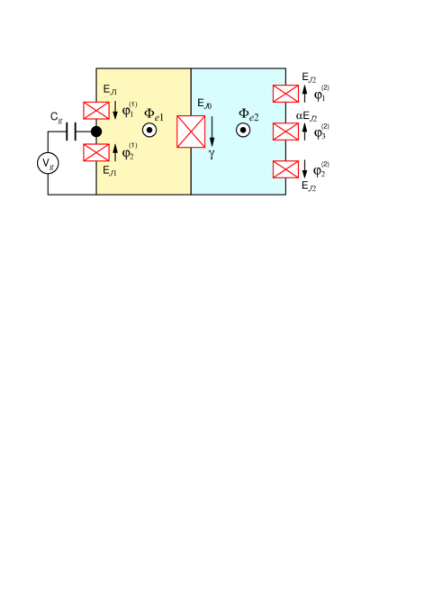
The hybrid quantum circuit we consider is shown in Fig. 1, where a charge qubit and a flux qubit is coupled by a large JJ. The phase drops across the JJs in the two qubits are coupled to the phase drop $\gamma$ across the large JJ:

$\displaystyle\varphi_{1}^{(1)}-\varphi_{2}^{(1)}-\gamma+2\pi f_{1}=0,$
$\displaystyle\varphi_{1}^{(2)}-\varphi_{2}^{(2)}+\varphi_{3}^{(2)}+\gamma+2\pi f_{2}=0,$ (1)

where the reduced magnetic fluxes are given by $f_{i}=\Phi_{ei}/\Phi_{0}$, with $i=1,2$. Here $\Phi_{0}$ is the magnetic flux quantum and $\Phi_{ei}$, $i=1,2$, are the magnetic fluxes applied to the charge and flux qubits, respectively. The Hamiltonian of the system is

$$H=H_{1}+H_{2}+H_{m}.$$ (2)

Here $H_{1}$ is the Hamiltonian of the charge qubit in the presence of the (middle) large JJ: JTNPRB

$$H_{1}=E_{c1}(n-n_{g})^{2}-2E_{J1}\cos\left(\pi f_{1}-\frac{1}{2}\gamma\right)\cos\varphi,$$ (3)

where $E_{c1}=e^{2}/C_{J}$ is the charging energy of the superconducting island in the charge qubit, $n=-i\partial/\partial\varphi$, $n_{g}=C_{g}V_{g}/2e$, and $\varphi=\frac{1}{2}(\varphi_{1}^{(1)}+\varphi_{2}^{(1)})$.

Refer to caption
Figure 1: (Color online) Schematic diagram of a hybrid quantum circuit with the charge (left) and flux (right) qubits connected to a large (middle) Josephson junction (JJ). In the charge qubit, the two JJs have the same Josephson coupling energy $E_{J1}$ and capacitance $C_{J}$. In the flux qubits, two JJs have the same Josephson coupling energy $E_{J2}$ and capacitance $C_{f}$; the third JJ has a smaller Josephson coupling energy $\alpha E_{J2}$ and capacitance $\alpha C_{f}$, where $0.5<\alpha<1$. The large JJ in the middle has the Josephson coupling energy $E_{J0}$ and capacitance $C_{0}$. For the ideal hybrid circuit, $E_{J0}\gg E_{J2}\gg E_{J1}$. Here the arrow near each JJ denotes the chosen direction for the positive phase drop across the corresponding junction.

The Hamiltonian of the flux qubit in the presence of the large JJ is given by Orlando

$\displaystyle H_{2}\!$ $\displaystyle\!=\!$ $\displaystyle\!\frac{P_{p}^{2}}{2M_{p}}+\frac{P_{q}^{2}}{2M_{q}}+2E_{J2}(1-\cos\varphi_{p}\cos\varphi_{q})$ (4)
$\displaystyle+\alpha E_{J2}\left[1-\cos\left(2\varphi_{q}+\gamma+2\pi f_{2}\right)\right],$

where

$\displaystyle P_{k}\!$ $\displaystyle\!=\!$ $\displaystyle\!-i\hbar{\partial}/{\partial\varphi_{k}},\,\,\,\,k=p,q,$
$\displaystyle M_{p}\!$ $\displaystyle\!=\!$ $\displaystyle\!2C_{f}\left({\Phi_{0}}/{2\pi}\right)^{2},$ (5)
$\displaystyle M_{q}\!$ $\displaystyle\!=\!$ $\displaystyle\!M_{p}(1+2\alpha).$

The redefined phases $\varphi_{p}$ and $\varphi_{q}$ are $\varphi_{p}=\frac{1}{2}(\varphi_{1}^{(2)}+\varphi_{2}^{(2)})$ and $\varphi_{q}=\frac{1}{2}(\varphi_{1}^{(2)}-\varphi_{2}^{(2)})$. The Hamiltonian of the middle large JJ reads

$$H_{m}=E_{c0}\left(N+\frac{1}{2}n_{g}\right)^{2}-E_{J0}\cos\gamma,$$ (6)

where $E_{c0}=(2e)^{2}/2C_{0}$ is the charging energy of the large JJ and $N=-i\partial/\partial\gamma$.

We expand the potential in each qubit Hamiltonian into a series. When the middle JJ that couples the charge and flux qubits is large enough, one can retain the terms up to the first order of $\gamma$ (cf. Ref. JTNPRB, ). The total Hamiltonian is then reduced to

$$H=H_{c}+H_{f}+H_{m}+H_{\rm int},$$ (7)

where $H_{c}\equiv H_{1}(\gamma=0)$ is the Hamiltonian of the charge qubit without coupling to the large JJ and $H_{f}\equiv H_{2}(\gamma=0)$ is the Hamiltonian of the flux qubit without coupling to the large JJ. The interaction Hamiltonian $H_{\rm int}$ bewteen the two qubits and the large JJ is

$$H_{\rm int}=-\frac{\Phi_{0}}{2\pi}(I_{1}+I_{2})\gamma,$$ (8)

where the circulating supercurrents in the (left) charge and (right) flux qubits are given, respectively, by

$\displaystyle I_{1}\!$ $\displaystyle\!=\!$ $\displaystyle\!I_{c1}\sin(\pi f_{1})\cos\varphi,$
$\displaystyle I_{2}\!$ $\displaystyle\!=\!$ $\displaystyle\!-\alpha I_{c2}\sin(2\varphi_{q}+2\pi f_{2}),$ (9)

with $I_{ci}=2\pi E_{Ji}/\Phi_{0}$, $i=1,2$.

When the charge states $|0\rangle$ and $|1\rangle$ are used as the basis states, the Hamiltonian $H_{c}$ can be reduced to (see, e.g., Refs. JTNPRL, and MAK, )

$$H_{c}=\varepsilon_{1}(V_{g})\sigma_{z}^{(1)}-\Delta_{1}\sigma_{x}^{(1)},$$ (10)

where

$\displaystyle\varepsilon_{1}(V_{g})\!$ $\displaystyle\!=\!$ $\displaystyle\!\frac{1}{2}E_{c1}(C_{g}V_{g}/e-1),$
$\displaystyle\Delta_{1}\!$ $\displaystyle\!=\!$ $\displaystyle\!E_{J1}\cos(\pi f_{1}).$ (11)

The two charge states $|0\rangle$ and $|1\rangle$ correspond to zero and one extra Cooper pairs in the superconducting island, respectively. The circulating supercurrent $I_{1}$ is reduced to

$$I_{1}=\frac{1}{2}I_{c1}\sin(\pi f_{1})\sigma_{x}^{(1)}.$$ (12)

Using the basis states $|\!\uparrow\rangle$ and $|\!\downarrow\rangle$ corresponding to the states with maximal clockwise and counter-clockwise persistent supercurrents in the flux qubit, one can reduce the Hamiltonian $H_{f}$ to (see, e.g., Ref. MAJER, )

$$H_{f}=\varepsilon_{2}(\Phi_{2})\sigma_{z}^{(2)}-\Delta_{2}\sigma_{x}^{(2)},$$ (13)

where

$$\varepsilon_{2}(\Phi_{2})=I_{p}\left(\Phi_{2}-\frac{1}{2}\Phi_{0}\right),$$ (14)

and $\Delta_{2}$ is the tunneling amplitude of the barrier in the double-well potential. The circulating supercurrent $I_{2}$ is reduced to

$$I_{2}=I_{p}\sigma_{z}^{(2)},$$ (15)

where $I_{p}$ is the maximal persistent supercurrent of the flux qubit.

The middle JJ connecting the charge and flux qubits behaves like a particle with mass $M_{0}=2(\Phi_{0}/2\pi)^{2}C_{0}$, trapped in a cosinoidal potential $-E_{J0}\cos\gamma$. Because this JJ is large, it can be approximately regarded as a harmonic oscillator:

$$H_{m}=\hbar\omega_{p}a^{\dagger}a,$$ (16)

with the plasma frequency

$$\omega_{p}=\frac{\sqrt{8E_{J0}E_{c0}}}{\hbar}.$$ (17)

The boson operator is defined as

$$a=(\xi/2)\gamma+i(1/2\xi)N,$$ (18)

with

$$\xi=\left(\frac{E_{J0}}{2E_{c0}}\right)^{1/4}.$$ (19)

Thus, the phase drop $\gamma$ can be written as

$$\gamma=\frac{1}{\xi}\,(a^{\dagger}+a).$$ (20)

Substituting Eq. (20) into the interaction Hamiltonian (8), one can write the total Hamiltonian of the hybrid circuit as

$$H=H_{0}+H_{\rm int},$$ (21)

where

$\displaystyle H_{0}\!$ $\displaystyle\!=\!$ $\displaystyle\!\varepsilon_{1}(V_{g})\,\sigma_{z}^{(1)}-\Delta_{1}\sigma_{x}^{(1)}$ (22)
$\displaystyle\!+\varepsilon_{2}(\Phi_{2})\,\sigma_{z}^{(2)}-\Delta_{2}\,\sigma_{x}^{(2)}+\hbar\omega_{p}\,a^{\dagger}a,$

and

$$H_{\rm int}=-\left(g_{10}\,\sigma_{x}^{(1)}+g_{20}\,\sigma_{z}^{(2)}\right)(a^{\dagger}+a),$$ (23)

with

$\displaystyle g_{10}\!$ $\displaystyle\!=\!$ $\displaystyle\!\left({\Phi_{0}}/{2\pi}\right)\left({I_{c1}}/{2\xi}\right)\sin(\pi f_{1}),$
$\displaystyle g_{20}\!$ $\displaystyle\!=\!$ $\displaystyle\!\left({\Phi_{0}}/{2\pi}\right)\left({I_{p}}/{\xi}\right).$ (24)

This total Hamiltonian is analogous to two qubits separately coupled to an optical mode in a quantum cavity.

III Effective inter-qubit coupling

Here we consider the case with the plasmon energy splitting $\hbar\omega_{p}$ much larger than the qubit energy splitting $\hbar\omega_{q}$. Now the rotation-wave approximation cannot be used since the condition $\omega_{p}+\omega_{q}\gg\omega_{p}-\omega_{q}$, required for the rotation-wave approximation, is not satisfied here. Below we show that an effective interaction between the two qubits can be generated. Actually, because the plasmon energy splitting is much larger than the energy splittings of the qubits, the harmonic oscillator can be assumed to remain in the ground state, irrespective of the coupling of the large JJ to the qubits. Therefore, an effective inter-qubit interaction is achieved by exchanging virtual bosons between the large JJ and the qubits.

In the interaction picture, the system evolves as

$$|\Psi(t)\rangle=U(t,0)|\Psi(0)\rangle,$$ (25)

where the evolution operator, up to second order, reads quantum

$\displaystyle U(t,0)\!$ $\displaystyle\!=\!$ $\displaystyle\!1+\frac{1}{i\hbar}\int_{0}^{t}V_{I}(t_{1})dt_{1}$ (26)
$\displaystyle\!+\left(\frac{1}{i\hbar}\right)^{2}\int_{0}^{t}dt_{1}\int_{0}^{t_{1}}V_{I}(t_{1})V_{I}(t_{2})dt_{2}\,.$

The interaction operator $V_{I}(t)$ is

$$V_{I}(t)=U_{0}^{{\dagger}}(t)H_{\rm int}U_{0}(t)$$ (27)

with $U_{0}(t)=\exp(-iH_{0}t)$.

Here we use the basis states:

$\displaystyle|\Psi_{1n}\rangle\equiv|g^{(1)},g^{(2)}\rangle\otimes|n\rangle,$
$\displaystyle|\Psi_{2n}\rangle\equiv|g^{(1)},e^{(2)}\rangle\otimes|n\rangle,$
$\displaystyle|\Psi_{3n}\rangle\equiv|e^{(1)},g^{(2)}\rangle\otimes|n\rangle,$
$\displaystyle|\Psi_{4n}\rangle\equiv|e^{(1)},e^{(2)}\rangle\otimes|n\rangle,$

where $|g^{(i)}\rangle$ and $|e^{(i)}\rangle$ are the ground and excited states of the qubit $i$ ($i=1,2$), and $|n\rangle$ corresponds to the state of the harmonic oscillator with $n$ bosons. Equation (26) can be written as

$\displaystyle U(t,0)\!$ $\displaystyle\!=\!$ $\displaystyle\!1+\frac{1}{i\hbar}\int_{0}^{t}F(t_{1})dt_{1}$ (28)
$\displaystyle\!+\left(\frac{1}{i\hbar}\right)^{2}\int_{0}^{t}dt_{1}\int_{0}^{t_{1}}G(t_{1},t_{2})dt_{2}\,,$

where

$$F(t_{1})=\sum_{i,m}|\Psi_{im}\rangle\langle\Psi_{im}|V_{I}(t_{1})\sum_{j,n}|\Psi_{jn}\rangle\langle\Psi_{jn}|\,,$$ (29)

and

$\displaystyle G(t_{1},t_{2})\!$ $\displaystyle\!=\!$ $\displaystyle\!\sum_{i,m}|\Psi_{im}\rangle\langle\Psi_{im}|V_{I}(t_{1})\sum_{j,n}|\Psi_{jn}\rangle\langle\Psi_{jn}|$ (30)
$\displaystyle\times V_{I}(t_{2})\sum_{k,p}|\Psi_{kp}\rangle\langle\Psi_{kp}|\,,$

with $i,j,k=1,2,3$ and 4, and $m,n,p=0,1,2,\dots$. After tedious calculations and neglecting the fast oscillatory terms, we have

$$U(t,0)\approx 1+\frac{1}{i\hbar}\int_{0}^{t}V_{\rm eff}\,dt_{1}\,,$$ (31)

where

$$V_{\rm eff}=\chi\,\sigma_{x}^{(1)}\sigma_{z}^{(2)},$$ (32)

with

$$\chi=\frac{2g_{10}g_{20}}{\hbar\omega_{p}}=\left(\frac{\Phi_{0}}{2\pi}\right)^{2}\frac{I_{c1}I_{p}\sin(\pi f_{1})}{2E_{J0}}.$$ (33)

The reduced interaction Hamiltonian $V_{\rm eff}$ corresponds to an effective coupling between the two qubits after eliminating the degree of freedom of the large JJ.

Converted to the Schödinger picture and neglecting the fast oscillatory terms, the total Hamiltonian is then reduced to

$\displaystyle H\!$ $\displaystyle\!=\!$ $\displaystyle\!\varepsilon_{1}(V_{g})\,\sigma_{z}^{(1)}-\Delta_{1}\sigma_{x}^{(1)}$ (34)
$\displaystyle\!+\varepsilon_{2}(\Phi_{2})\,\sigma_{z}^{(2)}-\Delta_{2}\,\sigma_{x}^{(2)}+\chi\,\sigma_{x}^{(1)}\sigma_{z}^{(2)}.$

It is interesting to note that the resulting inter-qubit coupling $\chi\,\sigma_{x}^{(1)}\sigma_{z}^{(2)}$ implies that the large JJ can behave like an inductance of value

$$L_{J}=\frac{\Phi_{0}}{2\pi I_{c0}},$$ (35)

where $I_{c0}=2\pi E_{J0}/\Phi_{0}$. To see this, one can directly use the expressions, Eqs. (12) and (15), of the circulating supercurrents $I_{i}$, $i=1,2$, for charge and flux qubits and calculate the inductive inter-qubit coupling using the inductance $L_{J}$:

$\displaystyle L_{J}I_{1}I_{2}\!$ $\displaystyle\!=\!$ $\displaystyle\!\frac{1}{2}L_{J}I_{c1}I_{p}\sin(\pi f_{1})\sigma_{x}^{(1)}\sigma_{z}^{(2)}$ (36)
$\displaystyle\equiv\!$ $\displaystyle\!\chi\sigma_{x}^{(1)}\sigma_{z}^{(2)}.$

This is just the inter-qubit coupling given in Eqs. (32)-(34). In particular, when $\Phi_{e1}=0$, the charge qubit has no loop current and the coupling between the charge and flux qubits is switched off.

IV Quantum memory

Below we show a typical two-qubit gate achieved using Hamiltonian (34). This gate is called iSWAP and can be conveniently used to transfer an arbitrary unknown state of the charge qubit to the flux qubit working at the optimal point.

Let $\Phi_{ei}=\frac{1}{2}\Phi_{0}$, with $i=1,2$, so that $\Delta_{1}(\Phi_{e1})=\varepsilon_{2}(\Phi_{e2})=0$. Moreover, we choose a suitable gate voltage $V_{g}$ to have $\varepsilon_{1}(V_{g})=-\Delta_{2}\equiv-\Delta$, The Hamiltonian (34) is reduced to

$$H=-\Delta\sigma_{z}^{(1)}-\Delta\sigma_{x}^{(2)}+\chi\sigma_{x}^{(1)}\sigma_{z}^{(2)}.$$ (37)

With the basis states $|0g\rangle$, $|1g\rangle$, $|0e\rangle$ and $|1e\rangle$, the two-qubit evolution operator $U=\exp(-iHt/\hbar)$ can be written as

$$U=\left(\begin{array}[]{cccc}a&0&0&d\\ 0&b&c&0\\ 0&c&b&0\\ d&0&0&a^{*}\end{array}\right),$$ (38)

where

$\displaystyle a\!$ $\displaystyle\!=\!$ $\displaystyle\!\cos(\Omega t)-i\frac{2\Delta\sin(\Omega t)}{\Omega},$
$\displaystyle b\!$ $\displaystyle\!=\!$ $\displaystyle\!\cos(\chi t),$
$\displaystyle c\!$ $\displaystyle\!=\!$ $\displaystyle\!-i\sin(\chi t),$
$\displaystyle d\!$ $\displaystyle\!=\!$ $\displaystyle\!-i\frac{2\chi\sin(\Omega t)}{\Omega},$ (39)

with $\Omega=(4\Delta^{2}+\chi^{2})^{1/2}$.

When $\cos(\Omega\tau)=1$ and $\sin(\chi\tau)=-1$, the two-qubit operation is an iSWAP gate:

$$U_{\rm iSWAP}=\left(\begin{array}[]{cccc}1&0&0&0\\ 0&0&i&0\\ 0&i&0&0\\ 0&0&0&1\end{array}\right).$$ (40)

This gate can be achieved by choosing $\Omega\tau=2n\pi$ and $\chi\tau=(2m-\frac{1}{2})\pi$, which requires that

$$\frac{\chi}{\Omega}=\frac{4m-1}{4n},$$ (41)

where $m,n=1,2,3,\dots$. For instance, $\chi/\Omega=1/8$ when $m=1$ and $n=6$, which gives $\chi/\Delta\approx 0.25$.

In order to transfer an arbitrary superposition state of the charge qubit to the flux qubit, we first prepare the flux qubit at the ground state $|g\rangle$ and then apply the iSWAP gate to the two-qubit system. This gives rise to

$$(\alpha|0\rangle+\beta|1\rangle)|g\rangle\Longrightarrow|0\rangle(\alpha|g\rangle+i\beta|e\rangle).$$ (42)

Furthermore, to convert $i\beta|e\rangle$ to $\beta|e\rangle$, one can just freely evolve the flux qubit for a time $t=\pi\hbar/4\Delta_{2}$ after the interaction with the charge qubit is switched off (by choosing $\Phi_{e1}=0$). This corresponds to applying a one-qubit rotation $\exp\left(i\Delta_{2}\sigma_{x}^{(2)}t/\hbar\right)$ on the flux qubit for the time $t=\pi\hbar/4\Delta_{2}$. After this free evolution of the flux qubit, one has

$$\alpha|g\rangle+i\beta|e\rangle\Longrightarrow(\alpha|g\rangle+\beta|e\rangle),$$ (43)

up to a global phase factor that produces no effect on the quantum state. Therefore, an arbitrary unknown state $\alpha|0\rangle+\beta|1\rangle$ of the charge qubit is finally transferred to the flux qubit as $\alpha|g\rangle+\beta|e\rangle$. Because the flux qubit works at the optimal point and it has a relatively long decoherence time, the above operations provide a promising way to achieve a quantum memory that stores the quantum information for a longer time in the flux qubit. Also, when needed, the quantum information stored in the flux qubit can be converted back to the charge qubit by just successively applying the above operations in the reverse manner.

Finally, we estimate the coupling strength between the charge and flux qubits. For instance, one can choose $E_{J0}=5E_{J2}$. Typically, the flux qubit has an energy splitting $\Delta_{2}\approx 0.02E_{J2}$ when $\alpha\approx 0.75$ and the maximal persistent supercurrent is $I_{p}\sim 0.5I_{c2}=\pi E_{J2}/\Phi_{0}$. If the Josephson coupling energies are chosen as $E_{J1}=0.04E_{J2}$ for both charge and flux qubits, the inter-qubit coupling strength is $\chi\sim 0.002E_{J2}$; when $E_{J1}=0.1E_{J2}$, $\chi\sim 0.005E_{J2}$. Thus, one has $\chi$ in the range of $0.6$ GHz $\sim 1.5$ GHz for a typical Josephson coupling energy $E_{J2}=300$ GHz. This inter-qubit coupling strength is strong enough for achieving a fast two-qubit operation used for the quantum memory. Moreover, for $\chi\sim 0.005E_{J2}$ and $\Delta\equiv\Delta_{2}\approx 0.02E_{J2}$, one has $\chi/\Delta\sim 0.25$, which corresponds to Eq. (41) with $m=1$ and $n=6$. This implies that the iSWAP gate is achievable by choosing suitable parameters for the hybrid quantum circuit.

V Conclusion

In conclusion, we have proposed a hybrid quantum circuit where both charge and flux qubits are connected to a large JJ. This large JJ gives rise to an effective inductive coupling between the charge and flux qubits, which is switchable via the magnetic flux applied to the charge qubit. Moreover, the resulting inter-qubit coupling can be used to transfer an arbitrary superposition state of the charge qubit to the flux qubit working at the optimal point. This hybrid circuit provides a promising quantum memory because the flux qubit at the optimal point can store the tranferred quantum state for a long time.

Acknowledgements.
This work was supported in part by the NSA, LPS and ARO. X.L.H. and J.Q.Y. were supported by the SRFDP, the NFRPC grant No. 2006CB921205 and the National Natural Science Foundation of China grant Nos. 10534060 and 10625416.

References

  • (1) J.Q. You and F. Nori, Phys. Today 58(11), 42 (2005), and references therein.
  • (2) Y. Nakamura, Yu.A. Pashkin, and J.S. Tsai, Nature (London) 398, 786 (1999).
  • (3) T.P. Orlando, J.E. Mooij, L. Tian, C.H. van der Wal, L.S. Levitov, S. Lloyd, and J.J. Mazo, Phys. Rev. B 60, 15398 (1999).
  • (4) P. Bertet, I. Chiorescu, G. Burkard, K. Semba, C.J.P.M. Harmans, D.P. DiVincenzo, and J.E. Mooij, Phys. Rev. Lett. 95, 257002 (2005).
  • (5) J. Q. You, J. S. Tsai, and F. Nori, Phys. Rev. Lett. 89, 197902 (2002); see also New Directions in Mesoscopic Physics, edited by R. Fazio, V.F. Gantmakher and Y. Imry (Kluwer, Dordrecht, 2003), pp. 351-360
  • (6) Y. Makhlin, G. Schön, and A. Shnirman, Nature (London) 398, 305 (1999).
  • (7) J.Q. You, J.S. Tsai, and F. Nori, Phys. Rev. B 68, 024510 (2003).
  • (8) J. Lantz, M. Wallquist, V.S. Shumeiko, and G. Wendin, Phys. Rev. B 70, 140507(R) (2004).
  • (9) J.Q. You, Y. Nakamura, and F. Nori, Phys. Rev. B 71, 024532 (2005); B.L.T. Plourde, J. Zhang, K.B. Whaley, F.K. Wilhelm, T.L. Robertson, T. Hime, S. Linzen, P.A. Reichardt, C.-E. Wu, and J. Clarke, Phys. Rev. B 70, 140501 (2004).
  • (10) A. Izmalkov, M. Grajcar, E. Il’ichev, Th. Wagner, H.-G. Meyer, A.Yu. Smirnov, M.H.S. Amin, A. Maassen van den Brink, and A.M. Zagoskin, Phys. Rev. Lett. 93, 037003 (2004).
  • (11) J.B. Majer, F.G. Paauw, A.C.J. ter Haar, C.J.P.M. Harmans, and J.E. Mooij, Phys. Rev. Lett. 94, 090501 (2005).
  • (12) C. Rigetti, A. Blais, and M. Devoret, Phys. Rev. Lett. 94, 240502 (2005).
  • (13) Y.X. Liu, L.F. Wei, J.S. Tsai, and F. Nori, Phys. Rev. Lett. 96, 067003 (2006); P. Bertet, C.J.P.M. Harmans, and J.E. Mooij, Phys. Rev. B 73, 064512 (2006); M. Grajcar, Y.X. Liu, F. Nori, and A.M. Zagoskin, Phys. Rev. B 74, 172505 (2006).
  • (14) See, e.g., E. Merzbacher, Quantum Mechanics, 3rd Ed. (John Wiley, New York, 1998), Chapt. 19; Y.X. Liu, L.F. Wei, and F. Nori, Phys. Rev. A 72, 033818 (2005).