Exact Potts Model Partition Functions for Strips of the Honeycomb Lattice

Abstract

We present exact calculations of the Potts model partition function $Z(G,q,v)$ for arbitrary $q$ and temperature-like variable $v$ on $n$-vertex strip graphs $G$ of the honeycomb lattice for a variety of transverse widths equal to $L_{y}$ vertices and for arbitrarily great length, with free longitudinal boundary conditions and free and periodic transverse boundary conditions. These partition functions have the form $Z(G,q,v)=\sum_{j=1}^{N_{Z,G,\lambda}}c_{Z,G,j}(\lambda_{Z,G,j})^{m}$, where $m$ denotes the number of repeated subgraphs in the longitudinal direction. We give general formulas for $N_{Z,G,j}$ for arbitrary $L_{y}$. We also present plots of zeros of the partition function in the $q$ plane for various values of $v$ and in the $v$ plane for various values of $q$. Explicit results for partition functions are given in the text for $L_{y}=2,3$ (free) and $L_{y}=4$ (cylindrical), and plots of partition function zeros are given for $L_{y}$ up to 5 (free) and $L_{y}=6$ (cylindrical). Plots of the internal energy and specific heat per site for infinite-length strips are also presented.

Key Words: Potts model, honeycomb lattice, exact solutions, transfer matrix

1 Introduction

In this paper we present some theorems on structural properties of Potts model partition functions on strips of the honeycomb ($hc$) lattice of arbitrary width equal to $L_{y}$ vertices and arbitrarily great length. We also report exact calculations of these partition functions for a number of honeycomb-lattice strips of various widths and arbitrarily great lengths. Using these results, we consider the limit of infinite length. For this limit we calculate thermodynamic functions and determine the loci in the complex $q$ and temperature planes where the free energy is non-analytic. This is an extension of our previous study for this lattice in [1].

We briefly review the definition of the model and relevant notation. Consider a graph $G=(V,E)$, defined by its vertex set $V$ and edge set $E$. (Here we keep the discussion general; shortly, we will specialize to strips of the honeycomb lattice.) Denote the number of vertices and edges as $|V|\equiv n$ and $|E|$, respectively. On the graph $G$, at temperature $T$, the Potts model is defined by the partition function $Z(G,q,v)=\sum_{\{\sigma_{n}\}}e^{-\beta{\cal H}}$ with the (zero-field) Hamiltonian ${\cal H}=-J\sum_{\langle ij\rangle}\delta_{\sigma_{i}\sigma_{j}}$ where $\sigma_{i}=1,\ldots,q$ are the spin variables on each vertex $i\in V$; $\beta=(k_{B}T)^{-1}$; $\langle ij\rangle\in E$ denotes pairs of adjacent vertices, and $J$ is the spin-spin interaction constant. We use the notation $K=\beta J$, $a=e^{K}$, and $v=e^{K}-1$. The physical ranges are thus (i) $a\geq 1$, i.e., $v\geq 0$ corresponding to $\infty\geq T\geq 0$ for the Potts ferromagnet with $J>0$, and (ii) $0\leq a\leq 1$, i.e., $-1\leq v\leq 0$, corresponding to $0\leq T\leq\infty$ for the Potts antiferromagnet with $J<0$. Let $G^{\prime}=(V,E^{\prime})$ with $E^{\prime}\subseteq E$. Then $Z(G,q,v)$ can be defined for arbitrary $q$ and $v$ by the formula [2]

$$Z(G,q,v)=\sum_{G^{\prime}\subseteq G}q^{k(G^{\prime})}v^{|E^{\prime}|}$$ (1.1)

where $k(G^{\prime})$ denotes the number of connected components of $G^{\prime}$. We define a (reduced) free energy per site $f=-\beta F$, where $F$ is the free energy, via

$$f(\{G\},q,v)=\lim_{n\to\infty}\ln[Z(G,q,v)^{1/n}]\ ,$$ (1.2)

where the symbol $\{G\}$ denotes $\lim_{n\to\infty}G$ for a given family of graphs $G$.

Our exact results on $Z(G,q,v)$ apply for arbitrary $q$ and $v$. We consider free and cylindrical strip graphs $G$ of the honeycomb lattice of width $L_{y}$ vertices and of arbitrarily great length $L_{x}$ vertices. Here, free boundary conditions (sometimes denoted FF), mean free in both the transverse and longitudinal directions (the latter being the one that is varied for a fixed width), while cylindrical boundary conditions (sometimes denoted PF) mean periodic in the transverse direction and free in the longitudinal direction. We represent the strip of the honeycomb lattice in the form of bricks oriented horizontally. For the honeycomb lattice with cylindrical boundary conditions, the number of vertices in the transverse direction, $L_{y}$, must be an even number, and the smallest value without degeneracy (multiple edges) is $L_{y}=4$. Exact partition functions for arbitrary $q$ and $v$ have previously been presented for strips of the honeycomb lattice with free boundary conditions for width $L_{y}=2$ in [1]. Our new results include theorems that describe the structure of the Potts model partition function for strips with free and cylindrical boundary conditions, of arbitrary width and length and explicit calculations using the transfer matrix method (in the Fortuin–Kasteleyn representation [3]) for strips with free and cylindrical boundary conditions with width $L_{y}=3$ (free) and $L_{y}=4$ (cylindrical). We have carried out similar calculations for $L_{y}\leq 7$ (free) and $L_{y}=6$ (cylindrical); these are too lengthy to include here. We shall also present plots of partition function zeros in the limit of infinite length, for widths $2\leq L_{y}\leq 5$ (free) and $L_{y}=4,6$ (cylindrical). Related calculations of Potts model partition functions for arbitrary $q$ and $v$ on fixed-width, arbitrary-length strips of the square and triangular lattices are [4]-[10] and [10, 11, 12], respectively. Analogous partition function calculations for arbitrary $q$ and $v$ on finite sections of 2D lattices with fixed width and length include [15, 16]. The special case $v=-1$ is the zero-temperature limit of the Potts antiferromagnet, for which $Z(G,q,-1)=P(G,q)$, where $P(G,q)$ is the chromatic polynomial expressing the number of ways of coloring the vertices of the graph $G$ with $q$ colors such that no two adjacent vertices have the same color.

As part of our work, we calculate zeros of the partition function in the $q$ plane for fixed $v$ and in the $v$ plane for fixed $q$. In the limit of infinite strip length, $L_{x}\to\infty$, there is a merging of such zeros to form continuous loci of points where the free energy is nonanalytic, which we denote generically as ${\cal B}$. For the limit $L_{x}\to\infty$ of a given family of strip graphs, this locus is determined as the solution to an algebraic equation and is hence an algebraic curve.

There are several motivations for this work. Clearly, exact calculations of Potts model partition functions with arbitrary $q$ and $v$ are of value in their own right. This is especially true since there are no exact calculations of the free energy $f(\{G\},q,v)$ for arbitrary $q$ and $v$ on an infinite lattice of dimension two or higher. Exact calculations on lattice strips of fixed width and arbitrarily great length thus provide a useful set of results complementing other methods of analysis such as series expansions and Monte Carlo simulations of the Potts model. Our structural theorems elucidate the form of the partition function on these strips for arbitrarily great widths as well as lengths. The honeycomb lattice is of interest since, together with the square and triangular lattices, it comprises the third and last regular tiling of the plane which is homopolygonal, i.e. composed of of a single type of regular polygon. While critical properties describing the second-order phase transition of the Potts ferromagnet are universal and independent of lattice type, the behavior of the Potts antiferromagnet is sensitively dependent on lattice type, so that studies of this model on different lattices and lattice strips are valuable.

There is a particular motivation for carrying out exact calculations of Potts model partition functions with arbitrary $q$ and $v$, because this allows one to investigate more deeply a unique feature of the model, which is qualitatively different from the behavior on either the square or triangular lattice, namely the property that the critical temperature of the Potts antiferromagnet on the honeycomb lattice decreases to zero, i.e., the critical $v$ decreases to $-1$, at a non-integral value, $q=(3+\sqrt{5})/2$ (as reviewed below in connection with the criticality condition, eq. (6.3)). This is formal, since for $q\not\in{\mathbb{Z}}_{+}$, the model (with either sign of $J$) is only defined via the representation (1.1), and in the antiferromagnet case (i.e., for $-1\leq v<0$), this formula can yield a negative, and hence unphysical, result for the partition function. One obviously cannot investigate this formal criticality using the Hamiltonian formulation, which requires $q\in{\mathbb{Z}}_{+}$.

Moreover, calculations of complex-temperature zeros of the partition function show how the physical phases can be generalized to regions in the plane of a complex-temperature variable, as was discussed for the 2D Ising model on the square lattice [13, 14]. Calculations of partition function zeros on long finite lattice strips, and the loci ${\cal B}$ in the infinite-length limit, also yield interesting insights into properties of the corresponding phase diagrams in the complex-temperature and complex-$q$ planes.

2 General Structural Theorems

2.1 Preliminaries

In this section we prove several general theorems that describe the structure of the partition function for the honeycomb-lattice strips under consideration. Let $m$ denote the number of bricks in the longitudinal direction for such a strip. Then the length (number of vertices in the longitudinal direction) is

$$L_{x}=\cases{2m+1&for odd $L_{x}$ \ ,\cr\cr 2m+2&for even $L_{x}$ \ .}$$ (2.1)

For this type of strip graph, $Z(G,q,v)$ has the form

$$Z(G,q,v)=\sum_{j=1}^{N_{Z,G,\lambda}}c_{G,j}(\lambda_{Z,G,j})^{m}$$ (2.2)

where the coefficients $c_{G,j}$ and corresponding terms $\lambda_{G,j}$, as well as the total number $N_{Z,G,\lambda}$ of these terms, depend on the type of strip (width and boundary conditions) but not on its length. In the special case $v=-1$, the numbers $N_{Z,G,\lambda}$ will be denoted $N_{P,G,\lambda}$. We define $N_{Z,hc,BC_{y}\ BC_{x},L_{y},\lambda}$ as the total number of $\lambda$’s for the honeycomb-lattice strip with the transverse and longitudinal boundary conditions $BC_{y}$ and $BC_{x}$ of width $L_{y}$. Henceforth where no confusion will result, we shall suppress the $\lambda$ subscript. The explicit labels are $N_{Z,hc,FF,L_{y}}$ and $N_{Z,hc,PF,L_{y}}$ for the strips of the honeycomb lattices with free and cylindrical boundary conditions.

2.2 Case of Free Boundary Conditions

Theorem 2.1

For arbitrary $L_{y}$,

$$N_{Z,hc,FF,L_{y}}=\cases{C_{L_{y}}&for odd $L_{y}$ \ ,\cr\cr\frac{1}{2}\left[C_{L_{y}}+{L_{y}\choose L_{y}/2}\right]&for even $L_{y}$ \ .}$$ (2.3)

Proof  A honeycomb-lattice strip with free boundary conditions is symmetric under reflection about the longitudinal axis if and only if $L_{y}$ is even. Therefore, for odd $L_{y}$, the total number of $\lambda$’s in the Potts model partition function, $N_{Z,hc,FF,L_{y}}$, is the same as the number for the triangular lattice strips $N_{Z,tri,FF,L_{y}}$, namely, the number of non-crossing partitions of the set $\{1,2,...,L_{y}\}$. This is the Catalan number [19, 20], $C_{L}=(L+1)^{-1}{2L\choose L}$. For even $L_{x}$, the reflection symmetry reduces $N_{Z,hc,FF,L_{y}}$ to the number for the square lattice strips $N_{Z,sq,FF,L_{y}}$, which was given in Theorem 5 of [7].  $\Box$ We list the first few values of $N_{Z,hc,FF,L_{y}}$ in Table 1.

Table 1: Numbers of $\lambda$’s for the Potts model partition function and chromatic polynomials for the strips of the honeycomb lattices having free boundary conditions and various widths $L_{y}$.

$L_{y}$	$N_{Z,hc,FF,L_{y}}$	$N_{P,hc,FF,L_{y}}$
2	2	1
3	5	3
4	10	5
5	42	19
6	76	25
7	429	145
8	750	194
9	4862	1230
10	8524	1590
11	58786	11139
12	104468	14681

We next discuss some combinatorics which will be used in our next theorem. Let us denote the elements in the $k$’th column of the $j$’th row of Pascal’s triangle as $P(j,k)$, with the value $P(j,k)={j\choose k}$  (the binomial coefficient). The relation between these elements is $P(j,k)=P(j-1,k-1)+P(j-1,k)$ with $P(0,0)=1$, $P(j,-1)=0$, and $P(j,k)=0$ for $j<k$. That is, each element is the sum of the two numbers immediately above it. For the reader’s convenience, we display the first few rows of Pascal’s triangle in Fig. 1. Now, $P(j,k)$ is the number of ways to place $k$ black beads and $j-k$ white beads in a line. Similarly, what is known as Losanitsch’s triangle [17] is given by the number of ways to put $j$ beads of two colors in a line, modulo reflection symmetry. We denote the entry in the $k$’th column of the $j$’th row of this triangle as $L(j,k)$. For reference, the sequence formed by reading the entries in this triangle (from left to right) by rows is listed as sequence $A034851$ in [17]. The relation between these entries is essentially the same as for Pascal’s triangle, except when $j$ is even and $k$ is odd:

$$L(j,k)=L(j-1,k-1)+L(j-1,k)-\delta_{j\ {\rm even},k\ {\rm odd}}{j/2-1\choose(k-1)/2}$$ (2.4)

where $\delta_{j\ {\rm even},k\ {\rm odd}}=1$ if $j$ is even and $k$ is odd and zero otherwise. For reference, the first few rows of Losanitsch’s triangle are shown in Fig. 2. Now form a new triangle by subtracting the entries in Losanitsch’s triangle from the corresponding entries in Pascal’s triangle, and denote its elements as $PL(j,k)$. The first few rows of this triangle are displayed in Fig. 3.

								1
							1		1
						1		2		1
					1		3		3		1
				1		4		6		4		1
			1		5		10		10		5		1
		1		6		15		20		15		6		1
	1		7		21		35		35		21		7		1
1		8		28		56		70		56		28		8		1

Figure 1: Pascal’s triangle.

								1
							1		1
						1		1		1
					1		2		2		1
				1		2		4		2		1
			1		3		6		6		3		1
		1		3		9		10		9		3		1
	1		4		12		19		19		12		4		1
1		4		16		28		38		28		16		4		1

Figure 2: Losanitsch’s triangle.

								0
							0		0
						0		1		0
					0		1		1		0
				0		2		2		2		0
			0		2		4		4		2		0
		0		3		6		10		6		3		0
	0		3		9		16		16		9		3		0
0		4		12		28		32		28		12		4		0

Figure 3: Triangle formed by subtraction of elements of Losanitsch’s triangle from corresponding elements of Pascal’s triangle.

The next theorem concerns the number of $\lambda$’s $N_{P,hc,FF,L_{y}}$ in the chromatic polynomial for the free $hc$ strip.

Theorem 2.2

For arbitrary $L_{y}$,

$$N_{P,hc,FF,L_{y}}=\cases{\sum_{i=0}^{(L_{y}-1)/2}M_{L_{y}-1-i}{(L_{y}-1)/2\choose i}&for odd $L_{y}$ \ ,\cr\cr\sum_{i=0}^{L_{y}/2-1}N_{P,sq,FF,L_{y}-i}{L_{y}/2-1\choose i}&\cr-\frac{1}{2}\sum_{i=1}^{L_{y}/2-2}PL(L_{y}/2-1,i)N_{P,FP,[(L_{y}+1-i)/2]}&for even $L_{y}$ \ .}$$ (2.5)

where $M_{L}$ is the Motzkin number [18], $N_{P,sq,FF,L_{y}}$ is the number of $\lambda$’s for the square lattice with free boundary conditions given in Theorem 2 of [7], $N_{P,FP,L_{y}}$ is the total number of $\lambda$’s for the square, triangular, or honeycomb lattices with cyclic boundary conditions given in eq.(5.2) of [20], and $PL(j,k)$ is the number given by the subtraction of the elements of Losanitsch’s triangle from the corresponding elements of Pascal’s triangle.

Proof  Consider odd strips widths $L_{y}$ first; for these, there is no reflection symmetry. For each transverse slice containing $L_{y}$ vertices of the honeycomb lattice with free boundary conditions, there are $(L_{y}-1)/2$ edges. Compared with the calculation of partitions for strips of the square lattice, the same numbers of edges are removed, such that the end vertices of each of these missing edges are allowed to have the same color. Firstly, all of the possible partitions for the triangular-lattice strip with free boundary conditions $N_{P,tri,FF,L_{y}}=M_{L_{y}-1}$ [19] are valid for the honeycomb lattice. Among $(L_{y}-1)/2$ missing edges, if one pair of end vertices has the same color, the number of partitions is given by $N_{P,tri,FF,L_{y}-1}$. As an example, for the $L_{y}=3$ slice of the honeycomb-lattice strip, there is an edge connecting vertices 1 and 2 and no edge connecting vertices 2 and 3. It follows that the set of partitions is comprised of $\{1,\delta_{1,3},\delta_{2,3}\}$ in the shorthand notation used in [7, 12]. Similarly, if two pairs of end vertices of missing edges separately have the same color, there are ${(L_{y}-1)/2\choose 2}$ choices for the locations of missing edges and the number of partitions for each choice is $N_{P,tri,FF,L_{y}-2}$. By including all the possible missing edges with the same color on their end vertices, the first line in eq. (2.5) is established for the honeycomb lattice with odd $L_{y}$.

For the honeycomb lattice with even $L_{y}$, reflection symmetry must be taken into account. We thus consider partitions with the transverse slice composed of edges connecting vertices 1 and 2, vertices 3 and 4, …, vertices $L_{y}-1$ and $L_{y}$. That is, there are $L_{y}/2$ edges in each slice and $L_{y}/2-1$ missing edges. Naively, one would expect that the number of partitions is $\sum_{i=0}^{L_{y}/2-1}N_{P,sq,FF,L_{y}-i}{L_{y}/2-1\choose i}$ by the above argument. However, this would actually involve an overcounting, because certain partitions with the same color on end vertices of missing edge(s) are equivalent under the reflection symmetry. For example, the $L_{y}=6$ strip of the honeycomb lattice has two missing edges, i.e., there is no edge between vertices 2 and 3, and between vertices 4 and 5. There are $N_{P,sq,FF,5}=7$ partitions if vertices 2 and 3 have the same color, and separately seven partitions if vertices 4 and 5 have the same color. Five partitions for the first case $\delta_{2,3}$, $\delta_{2,3}\delta_{1,6}$, $\delta_{2,3,5}$, $\delta_{2,3}\delta_{1,4,6}$ and $\delta_{2,3,5}\delta_{1,6}$ are equivalent under reflection to the following partitions for the second case: $\delta_{4,5}$, $\delta_{4,5}\delta_{1,6}$, $\delta_{2,4,5}$, $\delta_{4,5}\delta_{1,3,6}$, and $\delta_{2,4,5}\delta_{1,6}$. In general, the double-counted partitions are those symmetric partitions in $N_{P,sq,FF,L_{y}-i}$ such that $i$ pairs of end vertices of missing edges have the same color. This number of symmetric partitions is $\frac{1}{2}N_{P,FP,[(L_{y}+1-i)/2]}$, given as Theorem 1 in [7]. The double counting occurs when two choices of $i$ missing edges are reflection-symmetric to each other. This number of asymmetric choices of missing edges is given by $PL(j,k)$.  $\Box$ We list the first few values of $N_{P,hc,FF,L_{y}}$ for the honeycomb lattice with free boundary conditions in Table 1.

2.3 Case of Cylindrical Boundary Conditions

For the honeycomb lattice with cylindrical boundary condition, only strips with even $L_{y}$ can be defined. The number of $\lambda$’s can be reduced from the number of non-crossing partitions $N_{Z,tri,FF,L_{y}}=C_{L_{y}}$ with length-two rotational symmetry, and this first reduction will be denoted as $N_{Z,hc,PF,L_{y}}^{\prime}$. This number can be further reduced with reflection symmetry, and this further-reduced number will be denoted as $N_{Z,hc,PF,L_{y}}$. We list the first few relevant numbers in the Potts model partition function for the strips of the honeycomb lattices with cylindrical boundary conditions in Table 2.

Table 2: Numbers of $\lambda$’s in the Potts model partition function for the strips of the honeycomb lattices having cylindrical boundary conditions and various even $L_{y}$.

$L_{y}$	$N_{Z,tri,FF,L_{y}}$	$N_{Z,hc,PF,L_{y}}^{\prime}$	$N_{Z,hc,PF,L_{y}}$	$2N_{Z,hc,PF,L_{y}}$	$\frac{L_{y}}{2}N_{Z,hc,PF,L_{y}}^{\prime}$
				$-N_{Z,hc,PF,L_{y}}^{\prime}$	$-N_{Z,tri,FF,L_{y}}$
2	2	2	2	2	0
4	14	10	8	6	6
6	132	48	34	20	12
8	1430	378	224	70	82
10	16796	3364	1808	252	24
12	208012	34848	17886	924	1076

Lemma 2.1

For arbitrary even $L_{y}$,

$$\frac{L_{y}}{2}N_{Z,hc,PF,L_{y}}^{\prime}-N_{Z,tri,FF,L_{y}}=\sum_{{\rm even}\ d|L_{y};\ 1\leq d<L_{y}}\phi\left(\frac{L_{y}}{d}\right){2d\choose d}$$ (2.6)

where $d|L_{y}$ means that $d$ divides $L_{y}$, and $\phi(n)$ is the Euler totient function, equal to the number of positive integers not exceeding the positive integer $n$ and relatively prime to $n$.

Proof  Because the honeycomb-lattice strip has length-two rotational symmetry, the value $\frac{L_{y}}{2}N_{Z,hc,PF,L_{y}}^{\prime}$ must be larger than $N_{Z,tri,FF,L_{y}}$. For strips with cylindrical boundary conditions, partitions can be classified according to the periodicity $d$ modulo rotations. That is, a partition could be transformed back to itself when the $L_{y}$ vertices are rotated by length $d$, where $d$ denotes any of the positive integers that divide $L_{y}$. The number of partitions which have periodicity $d$ modulo these rotations was denoted as $2\alpha_{d}$ in the proof of Theorem 2.2 of [12], and is given by

$$2\alpha_{d}=\frac{1}{d}\sum_{d^{\prime}|d}\mu(d/d^{\prime}){2d^{\prime}\choose d^{\prime}}$$ (2.7)

where $\mu(n)$ is the Möbius function, defined as $\mu(n)=-1$ if $n$ is prime, $\mu(n)=0$ if $n$ has a square factor, and $\mu(n)=1$ for other $n$. Now the periodicity $d$ can be either odd or even. For a partition with odd periodicity $d$, the contribution to the excess of $(L_{y}/2)N_{Z,hc,PF,L_{y}}^{\prime}$ relative to $N_{Z,tri,FF,L_{y}}$ is $2\alpha_{d}(L_{y}/2-d)$. On the honeycomb-lattice strip with length-two rotational symmetry, a partition with even periodicity $d$ and its length-one rotation are not equivalent. Thus for a partition with even periodicity $d$ and its length-one rotated counterpart, the contribution is $2\alpha_{d}(L_{y}-d)$. We have

$$\frac{L_{y}}{2}N_{Z,hc,PF,L_{y}}^{\prime}-N_{Z,tri,FF,L_{y}} = \sum_{{\rm even}\ d|L_{y}}2\alpha_{d}(L_{y}-d)+\sum_{{\rm odd}\ d|L_{y}}2\alpha_{d}(\frac{L_{y}}{2}-d)$$ (2.8)

$$= \sum_{d|L_{y}}2\alpha_{d}(L_{y}-d)-\sum_{{\rm odd}\ d|L_{y}}\alpha_{d}L_{y}$$ (2.10)

$$= \sum_{d|L_{y};\ 1\leq d<L_{y}}\phi(L_{y}/d){2d\choose d}-\sum_{{\rm odd}\ d|L_{y}}\alpha_{d}L_{y}$$ (2.12)

where the last line follows from the proof of Theorem 2.2 in [12]. Using eq. (2.7) for the second summation in eq. (2.12) is

$$\sum_{{\rm odd}\ d|L_{y}}\alpha_{d}L_{y} = \sum_{{\rm odd}\ d|L_{y}}\frac{L_{y}}{2d}\sum_{d^{\prime}|d}\mu(d/d^{\prime}){2d^{\prime}\choose d^{\prime}}$$ (2.13)

$$= \sum_{{\rm odd}\ d^{\prime}|L_{y}}\sum_{{\rm odd}\ d|L_{y};d^{\prime}|d}\frac{L_{y}}{2d}\mu(d/d^{\prime}){2d^{\prime}\choose d^{\prime}}$$ (2.15)

$$= \sum_{{\rm odd}\ d^{\prime}|L_{y}}\frac{1}{2}{2d^{\prime}\choose d^{\prime}}\sum_{{\rm odd}\ d^{\prime\prime}|L_{y}^{\prime}}\frac{L_{y}^{\prime}}{d^{\prime\prime}}\mu(d^{\prime\prime})\ ,$$ (2.17)

where we change the variables to $d^{\prime\prime}=d/d^{\prime}$ and $L_{y}^{\prime}=L_{y}/d^{\prime}$. (This is given as sequence A062570 in [17].) The summation of $d^{\prime\prime}$ is

$$\sum_{{\rm odd}\ d^{\prime\prime}|L_{y}^{\prime}}\frac{L_{y}^{\prime}}{d^{\prime\prime}}\mu(d^{\prime\prime})=\phi(2L_{y}^{\prime})=2\phi(L_{y}/d^{\prime})\ ,$$ (2.18)

where that second identity follows because $L_{y}^{\prime}$ is even by the formula for the Euler totient function, $\phi(n)=n\prod_{{\rm prime}\ p|n}(1-1/p)$. Therefore, we find

$$\sum_{{\rm odd}\ d|L_{y}}\alpha_{d}L_{y}=\sum_{{\rm odd}\ d|L_{y}}\phi(L_{y}/d){2d\choose d}\ ,$$ (2.19)

and the proof is completed.  $\Box$

Lemma 2.2

For arbitrary even $L_{y}$,

$$2N_{Z,hc,PF,L_{y}}-N_{Z,hc,PF,L_{y}}^{\prime}=N_{Z,FP,\frac{L_{y}}{2}}$$ (2.20)

where $N_{Z,FP,L_{y}}={2L_{y}\choose L_{y}}$ is the total number of $\lambda$’s for the square or triangular or honeycomb lattices with cyclic boundary conditions, given in eq.(5.6) of [20].

Proof  We use the result in Theorem 2.1 of [12] that $2N_{Z,sq,PF,L_{y}}-N_{Z,tri,PF,L_{y}}=N_{Z,FP,\frac{L_{y}}{2}}$ for even $L_{y}$ is the number of partitions with both rotation and reflection symmetries. The partitions that do not have reflection symmetry appear once in $N_{Z,sq,PF,L_{y}}$ but twice (itself plus its mirror image) in $N_{Z,tri,PF,L_{y}}$, so that they do not contribute to $2N_{Z,sq,PF,L_{y}}-N_{Z,tri,PF,L_{y}}$. It was shown there that for even $L_{y}$, there are two classes of reflection symmetries, denoted as type I and type II. For type I partitions, the reflection axis does not go through any vertex; while for type II partitions, the reflection axis goes through two vertices. There are at least two partitions that belong to both type I and II classes, namely, the partitions 1 (identity) and $\delta_{1,2,...,L_{y}}$ (unique block). Denote the set of partitions of $N_{Z,tri,PF,L_{y}}$ as ${\bf P}_{Z,tri,PF,L_{y}}$, that of $N_{Z,hc,PF,L_{y}}^{\prime}$ as ${\bf P}_{Z,hc,PF,L_{y}}^{\prime}$, and that of $N_{Z,hc,PF,L_{y}}$ as ${\bf P}_{Z,hc,PF,L_{y}}$. For example, ${\bf P}_{Z,tri,PF,4}=\{1,\delta_{1,2,3,4},\delta_{1,2},\delta_{1,3},\delta_{1,2}\delta_{3,4},\delta_{1,3,4}\}$. As the cylindrical strip of the honeycomb lattice only has length-two rotation symmetry, $N_{Z,hc,PF,L_{y}}^{\prime}$ is larger than $N_{Z,tri,PF,L_{y}}$. The excess partitions in ${\bf P}_{Z,hc,PF,L_{y}}^{\prime}$ relative to ${\bf P}_{Z,tri,PF,L_{y}}$ can be obtained by making length-one rotations for certain partitions in ${\bf P}_{Z,tri,PF,L_{y}}$. For example, in addition to those in ${\bf P}_{Z,tri,PF,L_{y}}$, ${\bf P}_{Z,hc,PF,4}^{\prime}$ contains $\delta_{2,3},\delta_{2,4},\delta_{2,3}\delta_{1,4},\delta_{1,2,4}$. Notice that the partitions that belong to both type I and II classes remain the same after the length-one rotation (modulo length-two rotational symmetry), so that they should be excluded in the doubling. For the honeycomb lattice, the reduction from ${\bf P}_{Z,hc,PF,L_{y}}^{\prime}$ to ${\bf P}_{Z,hc,PF,L_{y}}$ occurs only for type I partitions. Considering the $L_{y}=4$ strip again as an example, we observe that $\delta_{1,3}$ and $\delta_{2,4}$ are equivalent, so that only one of them should be kept for ${\bf P}_{Z,hc,PF,L_{y}}$, and similarly for $\delta_{1,3,4}$ and $\delta_{1,2,4}$. Since the numbers of partitions in type I and II classes are the same, the right hand side of eq. (2.20) is the same as that in Theorem 2.1 of [12] for even $L_{y}$.  $\Box$

The exact formula for $N_{Z,hc,PF,L_{y}}$ follows from Lemmas 2.1 and 2.2:

Theorem 2.3

For arbitrary even $L_{y}$,

$$N_{Z,hc,PF,L_{y}}=\frac{1}{2}{L_{y}\choose L_{y}/2}+\frac{1}{L_{y}}\left[C_{L_{y}}+\sum_{{\rm even}\ d|L_{y};\ 1\leq d<L_{y}}\phi\left(\frac{L_{y}}{d}\right){2d\choose d}\right]\ .$$ (2.21)

We list the first few relevant numbers in the chromatic polynomial for the strips of the honeycomb lattices with cylindrical boundary conditions in Table 3. Analogously to Lemmas 2.1 and 2.2, we state the following conjectures,

Table 3: Numbers of $\lambda$’s for the chromatic polynomial for the strips of the honeycomb lattices having cylindrical boundary conditions and various even $L_{y}$.

$L_{y}$	$n_{P}(hc,L_{y},0)$	$N_{P,hc,PF,L_{y}}^{\prime}$	$N_{P,hc,PF,L_{y}}$	$2N_{P,hc,PF,L_{y}}$	$\frac{L_{y}}{2}N_{P,hc,PF,L_{y}}^{\prime}$
				$-N_{P,hc,PF,L_{y}}^{\prime}$	$-n_{P}(hc,L_{y},0)$
2	1	1	1	1	0
4	6	5	4	3	4
6	43	17	12	7	8
8	352	99	62	25	44
10	3114	626	346	66	16
12	29004	4907	2576	245	438

Conjecture 2.1

For arbitrary even $L_{y}$,

$$\frac{L_{y}}{2}N_{P,hc,PF,L_{y}}^{\prime}-n_{P}(hc,L_{y},0)=\sum_{{\rm even}\ d|L_{y};\ 1\leq d<L_{y}}\phi\left(\frac{L_{y}}{d}\right)N_{P,hc,FP,d}$$ (2.22)

where $n_{P}(hc,L_{y},0)$ is the number of $\lambda$’s for the cyclic strips of the honeycomb lattice with level $d=0$, and $N_{P,hc,FP,L_{y}}$ is the total number of $\lambda$’s for these strips given in [1].

Compared with Lemma 2.1, the number of non-crossing partitions $N_{Z,tri,FF,L_{y}}=C_{L_{y}}$ is now replaced by the corresponding number $n_{P}(hc,L_{y},0)$ for the honeycomb strip in the chromatic polynomial, and the number ${2d\choose d}=N_{Z,hc,FP,d}$ is replaced by $N_{P,hc,FP,d}$.

Conjecture 2.2

For arbitrary even $L_{y}$,

$$2N_{P,hc,PF,L_{y}}-N_{P,hc,PF,L_{y}}^{\prime}=\cases{\frac{1}{2}N_{P,hc,FP,\frac{L_{y}}{2}}&for odd $L_{y}/2>1$ \ ,\cr\cr\frac{1}{2}\left[N_{P,hc,FP,\frac{L_{y}}{2}}+N_{P,hc,FP,\frac{L_{y}-2}{2}}\right]&for even $L_{y}/2$ \ .}$$ (2.23)

Conjectures 2.1 and 2.2 imply an exact formula for $N_{P,hc,PF,L_{y}}$.

3 Potts Model Partition Functions for Strips of the Honeycomb Lattice with Free Boundary Conditions

The Potts model partition function for a strip of the honeycomb lattice of width $L_{y}$ and length $L_{x}$ vertices with free boundary conditions is given by

$$Z(L_{y}\times L_{x},FF,q,v)={\bf w}^{\rm T}\cdot{\mathsf{T}}^{m}\cdot{\bf u}_{\rm id}$$ (3.1)

where ${\mathsf{T}}={\mathsf{V}}\cdot{\mathsf{H}}_{2}\cdot{\mathsf{V}}\cdot{\mathsf{H}}_{1}$ is the transfer matrix. ${\mathsf{H}}_{1}$ and ${\mathsf{H}}_{2}$ are matrices corresponding respectively to adding two kinds of transverse bonds in a slice, and ${\mathsf{V}}$ corresponding to adding longitudinal bonds in each slice. The number $m$ is related to $L_{x}$ as defined in eq. (2.1), and the vector $w$ is given by

$${\bf w}^{\rm T}=\cases{{\bf w}^{\rm T}_{\rm odd}={\bf v}^{\rm T}\cdot{\mathsf{H}}_{1}&for odd $L_{x}$ \ ,\cr\cr{\bf w}^{\rm T}_{\rm even}={\bf v}^{\rm T}\cdot{\mathsf{H}}_{2}\cdot{\mathsf{V}}\cdot{\mathsf{H}}_{1}&for even $L_{x}$ \ .}$$ (3.2)

Hereafter we shall follow the notation and the computational methods of [7, 12].

The matrices ${\mathsf{T}}$, ${\mathsf{V}}$, ${\mathsf{H}}_{1}$ and ${\mathsf{H}}_{2}$ act on the space of connectivities of sites on the first slice, whose basis elements ${\bf v}_{\cal P}$ are indexed by partitions ${\cal P}$ of the vertex set $\{1,\ldots,L_{y}\}$. In particular, ${\bf u}_{\rm id}={\bf v}_{\{\{1\},\{2\},\ldots,\{L_{y}\}\}}$. We denote the set of basis elements for a given strip as ${\bf P}=\{{\bf v}_{\cal P}\}$.

An equivalent way to present a general formula for the partition function is via a generating function. Labelling a lattice strip of a given type and width as $G_{m}$, with $m$ the length, one has

$$\Gamma(G,q,v,z)=\sum_{m=0}^{\infty}z^{m}Z(G_{m},q,v)$$ (3.3)

where $\Gamma(G,q,v,z)$ is a rational function

$$\Gamma(G,q,v,z)=\frac{{\cal N}(G,q,v,z)}{{\cal D}(G,q,v,z)}$$ (3.4)

with

$${\cal N}(G,q,v,z)=\sum_{j=0}^{\deg_{z}({\cal N})}A_{G,j}z^{j}$$ (3.5)

$${\cal D}(G,q,v,z)=1+\sum_{j=1}^{N_{Z,hc,BC,L_{y}}}b_{G,j}z^{j}=\prod_{j=1}^{N_{Z,hc,BC,L_{y}}}(1-\lambda_{Z,G,j}z)$$ (3.6)

where the subscript $BC$ denotes the boundary conditions. In the transfer-matrix formalism, the $\lambda_{Z,G,j}$’s in the denominator of the generating function, eq. (3.6), are the eigenvalues of ${\mathsf{T}}$.

Strips of the honeycomb lattice with free boundary conditions are well-defined for widths $L_{y}\geq 2$. The partition function $Z(G,q,v)$ was calculated, for arbitrary $q$, $v$, and $m$, for the strip with $L_{y}=2$ and free boundary conditions in [1], using a systematic iterative application of the deletion-contraction theorem. Here after re-expressing the results for $L_{y}=2$ in the present transfer matrix formalism, we shall report explicit results for the partition function for strips with $L_{y}=3$ and free boundary conditions. For $4\leq L_{y}\leq 7$, the expressions for ${\mathsf{T}}(L_{y})$, ${\bf w}(L_{y})$ and ${\bf u}_{\rm id}(L_{y})$ are too lengthy to include here. They are available from the authors on request.

3.1 $L_{y}=2$

For the strip with width $L_{y}=2$, we only have to consider odd $L_{x}$. The number of elements in the basis is equal to $C_{2}=2$: ${\bf P}=\{1,\delta_{1,2}\}$. In this basis, the transfer matrix and the other relevant quantities are given by

$${\mathsf{T}}&=\left(\begin{array}[]{cc}R_{11}&D_{1}F_{2}R_{12}\\ v^{5}&v^{4}D_{1}\end{array}\right)\\ {\bf w}_{\rm odd}^{\rm T}=q\left(F_{1},D_{1}\right)$$ (3.7)

where

$${}D_{k}&=v+k\\ {}F_{k}=q+kv\\ {}R_{11}=q^{4}+5q^{3}v+10q^{2}v^{2}+10qv^{3}+5v^{4}\\ R_{12}=q^{2}+2qv+2v^{2}\ .$$ (3.8)

In terms of this transfer matrix and these vectors, one calculates the partition function $Z(G_{m},q,v)$ for the strip with a given length $m$ via eq. (3.1). Equivalently, one can calculate the partition function using a generating function, and this was the way in which the results were presented in [1], with ${\cal D}=\prod_{j=1}^{2}(1-\lambda_{hcf2,j}z)$ and

$$\lambda_{hcf2,(1,2)}=\frac{1}{2}\biggl{[}M_{1}\pm\sqrt{M_{2}}\ \biggr{]}$$ (3.9)

where

$$M_{1}=q^{4}+5q^{3}v+10q^{2}v^{2}+10qv^{3}+6v^{4}+v^{5}$$ (3.10)

and

$$M_{2} = q^{8}+10q^{7}v+45q^{6}v^{2}+120q^{5}v^{3}+208q^{4}v^{4}-2q^{4}v^{5}+244q^{3}v^{5}-6q^{3}v^{6}$$ (3.13)

$$+196q^{2}v^{6}-4q^{2}v^{7}+104qv^{7}+4qv^{8}+32v^{8}+8v^{9}+v^{10}\ .$$

The product of these eigenvalues, i.e., the determinant of ${\mathsf{T}}$, is

$${\rm det}({\mathsf{T}})=v^{4}(1+v)(v+q)^{4}=v^{4}D_{1}F_{1}^{4}\ .$$ (3.14)

The vanishing of this determinant at $v=-1$ and $v=-q$ occurs because in each case one of the two eigenvalues is absent for, respectively, the chromatic and flow polynomials [21, 22]. Analogous formulas can be given for ${\rm det}({\mathsf{T}})$ for higher values of $L_{y}$; we omit these for brevity.

3.2 $L_{y}=3$

For the $hc$ strip of width $L_{y}=3$ the number of elements in the basis for enumerating partitions is given by the Catalan number $C_{3}=5$. This basis is ${\bf P}=\{1,\delta_{1,2},\delta_{1,3},\delta_{2,3},\delta_{1,2,3}\}$. In this basis, the transfer matrices and the other relevant quantities are

$${\mathsf{T}}&=\left(\begin{array}[]{ccccc}F_{1}F_{2}S_{11}&D_{1}F_{1}S_{12}&S_{13}S_{13}^{\prime}&S_{14}&D_{1}S_{15}\\ v^{5}F_{1}F_{2}&v^{4}D_{1}F_{1}F_{2}&v^{5}S_{23}&v^{5}S_{25}&v^{4}D_{1}S_{25}\\ v^{6}F_{1}&v^{5}D_{1}F_{1}&v^{4}S_{33}&v^{5}S_{25}&v^{4}D_{1}S_{25}\\ v^{3}F_{1}F_{2}R_{12}&v^{3}D_{1}F_{1}S_{42}&v^{3}F_{2}S_{43}&v^{3}S_{44}&v^{3}D_{1}S_{45}\\ v^{7}F_{1}&v^{6}D_{1}F_{1}&v^{6}S_{25}&v^{7}D_{3}&v^{6}D_{1}D_{3}\\ \end{array}\right)\\ {\bf w}_{\rm odd}^{\rm T}=q\left(q(q+v),q(1+v),q+v,q+v,1+v\right)\\ {\bf w}_{\rm even}^{\rm T}=q\left(F_{1}^{5},D_{1}F_{1}^{4},F_{1}X_{1},F_{1}^{2}X_{2},D_{1}F_{1}X_{2}\right)\\ {\bf u}_{\rm id}^{\rm T}=\left(1,0,0,0,0\right)$$ (3.15)

where the $S_{ij}$ and $X_{k}$ are defined in a shorthand notation as

$$S_{11}&=q^{4}+5q^{3}v+11q^{2}v^{2}+12qv^{3}+7v^{4}\\ S_{12}=q^{4}+6q^{3}v+15q^{2}v^{2}+19qv^{3}+11v^{4}\\ S_{13}=q^{2}+4qv+5v^{2}\\ S_{13}^{\prime}=q^{3}+4q^{2}v+7qv^{2}+7v^{3}+v^{4}\\ S_{14}=q^{5}+8q^{4}v+28q^{3}v^{2}+q^{3}v^{3}+54q^{2}v^{3}+5q^{2}v^{4}+59qv^{4}+9qv^{5}+32v^{5}+7v^{6}\cr\\ S_{15}=q^{4}+7q^{3}v+21q^{2}v^{2}+q^{2}v^{3}+33qv^{3}+4qv^{4}+24v^{4}+5v^{5}\\ S_{23}=2q+5v+v^{2}\\ S_{25}=q+4v+v^{2}\\ S_{33}=q^{2}+4qv+6v^{2}+v^{3}\\ S_{42}=q^{2}+3qv+3v^{2}\\ S_{43}=q^{2}+3qv+5v^{2}+v^{3}\\ S_{44}=q^{3}+6q^{2}v+q^{2}v^{2}+12qv^{2}+3qv^{3}+10v^{3}+3v^{4}\\ S_{45}=q^{2}+5qv+qv^{2}+7v^{2}+2v^{3}$$ (3.16)

$$X_{1}&=q^{3}+4q^{2}v+6qv^{2}+4v^{3}+v^{4}\\ X_{2}=q^{2}+3qv+3v^{2}+v^{3}$$ (3.17)

We will discuss properties of the resultant partition functions below.

4 Potts Model Partition Functions for Honeycomb-lattice Strips with Cylindrical Boundary Conditions

For the honeycomb lattice with cylindrical boundary conditions, the width must be even (and larger than two in order to avoid the degenerate situation of vertical edges forming emanating from and returning to a given vertex). The Potts model partition function $Z(G,q,v)$ for a honeycomb-lattice strip with cylindrical boundary conditions can be written in the same form as in eq.(3.1). Here either ${\mathsf{H}}_{1}$ or ${\mathsf{H}}_{2}$ should include the bond connecting the boundary sites in the transverse direction. The dimension of the transfer matrix can be reduced by the two symmetries discussed in Section 2, namely the length-two translation symmetry along the transverse direction and reflection symmetry. This number is $N_{Z,hc,PF,L_{y}}$ and is given in terms of $L_{y}$ by eq. (2.21) (see Table 2 for some numerical values). We consider the basis in the translation-invariant and reflection-invariant subspace to construct the transfer matrix and the corresponding vectors. To simplify the notation, we will still use ${\mathsf{T}}$, ${\bf w}$ and ${\bf u}_{\rm id}$ as in eq.(3.1), so that the partition function is given by the analogous equation, $Z(L_{y}\times L_{x},PF,q,v)={\bf w}^{\rm T}\cdot{\mathsf{T}}^{m}\cdot{\bf u}_{\rm id}$. We have calculated the transfer matrix ${\mathsf{T}}(L_{y})$ and the vectors ${\bf w}(L_{y})$ and ${\bf u}_{\rm id}(L_{y})$ for $L_{y}=4$ and $L_{y}=6$. The explicit results for $L_{y}=4$ are given in the appendix; the results for $L_{y}=6$ are too lengthy to present here, and are available upon request.

5 Partition Function Zeros in the $q$ Plane

In this section we shall present results for zeros in the $q$-plane for the partition function of the Potts antiferromagnet on strips of the honeycomb lattice with free and cylindrical boundary conditions, for various values of the temperature-like variable $v$. Fig. 4 shows these zeros for strips of widths $2\leq L\leq 5$ and free boundary conditions. In the limit $L_{x}\to\infty$ the zeros merge to form sets of curves which, together, comprise the locus ${\cal B}$. As an illustration of this, in Fig. 5 we show these zeros for the free strips of width $L_{y}=3$, together with the loci ${\cal B}$ for various values of $v$. One sees that the strip lengths that we use to calculate the zeros are sufficiently great that most of these zeros lie rather close to the infinite-length asymptotic loci. This behavior - that partition function zeros calculated for long strips generally lie close to the asymptotic loci ${\cal B}$ - is similar to what we found in our previous work. Hence, one can draw a reasonably good inference for many of the features of these loci ${\cal B}$ from the zeros. The corresponding partition-function zeros for honeycomb-lattice strips with $L_{y}=4,6$ and cylindrical boundary conditions are shown in Figure 6. Again, one could calculate the asymptotic loci ${\cal B}$, but since the zeros already give a reasonably good idea of the structure of these loci, they will suffice for our present purposes. Our Figs. 4 and 6 include calculations up to $L_{y}$=5 and 6, respectively. We previously studied the case $L_{y}=2$ in [1] (again for arbitrary $q$ and temperature). From our present results, we see that, for general values of $v$, as the width $L_{y}$ increases, the curve envelope moves outward somewhat and the arc endpoints on the left move slowly toward $q=0$. This behavior is consistent with the hypotheses that for a given $v$, as $L_{y}\to\infty$, (i) ${\cal B}_{q}$ would approach a limiting locus as $L_{y}\to\infty$ and (ii) this locus would separate the $q$ plane into different regions, with a curve passing through $q=0$ as well as a maximal real value, $q_{c}(v)$. This is qualitatively similar to the behavior that was found earlier for the square-lattice strips [4, 5, 7] and the triangular-lattice strips [12]. As expected, the convergence to the limit $L_{y}\to\infty$ seems to be faster with cylindrical boundary conditions, as there are no surface effects when the length is made infinite. In this limit $L_{y}\to\infty$, one expects that the locus ${\cal B}$ will have the property that the maximal point at which it crosses the real axis, $q_{c}(v)$, is equal to the solution, eq. (6.9) (with the plus sign for the square root), of the criticality condition on the infinite honeycomb lattice, eq. (6.3) below.

We recall some results for the special case $v=-1$ corresponding to the zero-temperature Potts antiferromagnet. Chromatic zeros were calculated for a finite patch of the honeycomb lattice with free and cylindrical boundary conditions in (Fig. 8 of) [23]. Chromatic zeros and asymptotic loci for strips of this lattice were calculated for free longitudinal boundary conditions in [1, 21, 24] and for periodic longitudinal boundary conditions in [1, 20, 25, 26] (see, e.g., Fig. 6 of [24] for $L_{y}=3$ and free b.c., Fig. 1 of [25] for $L_{y}=2$ and cyclic b.c., Fig. 17 of [1] and Fig. 7 of [26] for $L_{y}=3$ and cyclic b.c., and Figs. 8 and 9 of [26] for $L_{y}=4$ and $L_{y}=5$ with cyclic b.c.). Comparisons of the arcs on ${\cal B}$ for $v=-1$ obtained for strips with free longitudinal boundary conditions led to the inference that in the limit $L_{y}\to\infty$ these loci would separate the $q$ plane into regions including a curve passing through $q=0$ [29]. The property that, for $v=-1$, ${\cal B}_{q}$ separates the $q$ plane into regions with one of the curves on ${\cal B}_{q}$ passing through the origin is also observed for lattice strips with finite width $L_{y}$ if one imposes periodic longitudinal boundary conditions [25],[27]-[29]. In particular, for $v=-1$ and cyclic b.c., we found the following values of $q_{c}(-1)$ (i) 2 for $L_{y}=2$ [25], (ii) 2 for $L_{y}=3$ [1], (iii) $\simeq 2.1548$ for $L_{y}=4$ [26], and (iv) $\simeq 2.2641$ for $L_{y}=5$ [26]. For $L_{y}\to\infty$, eq. (6.9) formally yields $q_{c}(-1)=(3+\sqrt{5})/2\simeq 2.6180$. This is formal since the Potts antiferromagnet is, in general, only defined for $q\in{\mathbb{Z}}_{+}$, owing to the fact that the formula (1.1) can yield a negative and hence unphysical value for $Z(G,q,v)$ if $v$ is negative and $q$ is not a non-negative integer. There are at least two different ways in which, as $L_{y}\to\infty$, the loci ${\cal B}$ could approach the limiting form containing $q_{c}(-1)$: (i) the endpoints of the complex-conjugate prongs farthest to the right could move down and pinch the real axis and/or (ii) the point at which the locus ${\cal B}$ for finite $L_{y}$ crosses the real axis could increase to this limiting value. These are not necessarily mutually exclusive; a combination of (i) and (ii) could presumably occur, so that the final locus would have a structure similar to that of the $L_{y}=2$ cyclic case shown in Fig. 1(a) of [25] or the $L_{y}=3$ case shown in Fig. 7 of [26], in which several curves on ${\cal B}$ meet at $q_{c}(-1)$. Alternatively, the rightmost complex-conjugate prongs might bend back and intersect the rest of the boundary ${\cal B}$ away from the real axis, forming “bubble” regions, as we found for the cyclic $L_{y}=4,5$ strips (Figs. 8 and 9 in [26]).

As regards the general distribution of zeros, for a given $L_{y}$, as $v$ increases from $-1$ to 0 (i.e., $K=\beta J$ increases from $-\infty$ to 0, these zeros contract to a point at $q=0$. This is an elementary consequence of the fact that $K\to 0$, the spin-spin interaction term in the Potts model Hamiltonian, ${\cal H}$, vanishes, so that the sum over states just counts all $q$ possible spin states independently at each vertex, and $Z(G,q,v)$ approaches the value $Z(G,q,0)=q^{n}$. More generally, one can inquire about the maximum modulus of a zero of $Z(G,q,v)$ in the $q$ plane as a function of $v$. It has been proved [30] that (for a graph $G$ without loops), for the antiferromagnetic Potts model partition function with $|1+v|\leq 1$, the zeros of $Z(G,q,v)$ lie in the disk $|q|<Cr|v|$, where $C\simeq 7.964$ and $r$ is the maximal degree of a vertex, with $r=3$ for our honeycomb-lattice strips. Our zeros have moduli that lie considerably below this upper bound. For example, for $v=-1$, the zeros that we have calculated and displayed in Figs. 4-6 have moduli bounded above by about 1.2 and 1.3, respectively, while the above-mentioned inequality would give an upper bound of $|q|<3C\simeq 23.9$.

One can also plot ${\cal B}_{q}$ for the ferromagnetic region $0\leq v\leq\infty$. Although we have not included these plots here, we note that an elementary Peierls argument shows that the Potts ferromagnet on infinite-length, finite-width strips has no finite-temperature phase transition and associated magnetic long range order. Hence, for this model ${\cal B}_{q}$ does not cross the positive real $q$ axis for $0<v<\infty$.

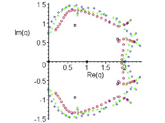
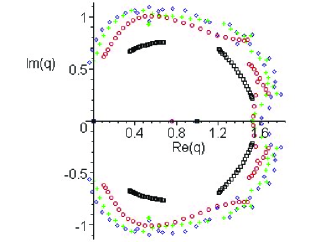
(((a)(a)	(((a)(b)
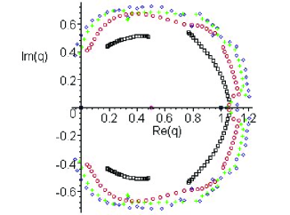
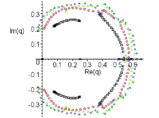
(((a)(c)	(((a)(d)

Figure 4: Partition-function zeros in the $q$ plane for the Potts antiferromagnet with (a) $v=-1.0$, (b) $v=-0.75$, (c) $v=-0.5$, and (d) $v=-0.25$ on strips with free boundary conditions and several widths $L_{y}$: 2 ($\Box$, black), 3 ($\circ$, red), 4 ($+$, green), and 5 ($\Diamond$, blue), where the colors refer to the online paper.

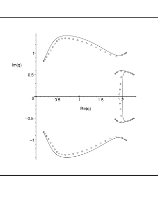
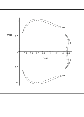
(((a)(a)	(((a)(b)
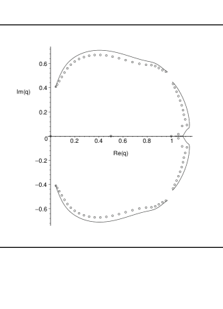
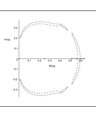
(((a)(c)	(((a)(d)

Figure 5: Partition-function zeros and asymptotic loci ${\cal B}$ in the $q$ plane for the Potts antiferromagnet on the $hc$ strip with width $L_{y}=3$ and free boundary conditions, for (a) $v=-1.0$, (b) $v=-0.75$, (c) $v=-0.5$, (d) $v=-0.25$.

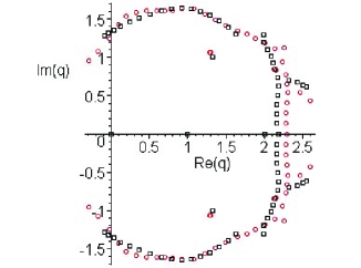
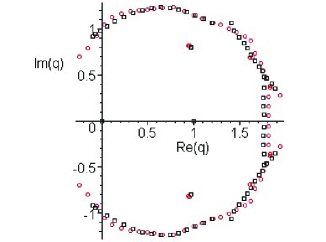
(((a)(a)	(((a)(b)
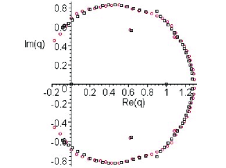
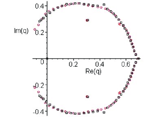
(((a)(c)	(((a)(d)

Figure 6: Partition-function zeros for (a) $v=-1.0$, (b) $v=-0.75$, (c) $v=-0.5$, and (d) $v=-0.25$ on strips with cylindrical boundary conditions and several widths $L_{y}$: 4 ($\Box$, black), 6 ($\circ$, red), where the colors refer to the online paper.

6 Partition Function Zeros in the $v$ Plane

6.1 General

In this section we shall present results for zeros in the $v$-plane, for various values of $q$, for the partition function of the Potts model on strips of the honeycomb lattice of widths $L_{y}\leq 5$ with free boundary conditions and of widths $L_{y}=4,6$ with cylindrical boundary conditions. We recall the possible noncommutativity in the definition of the free energy for certain special integer values of $q$, denoted $q_{sp}$, (see eqs. (2.10), (2.11) of [4]):

$$\lim_{n\to\infty}\lim_{q\to q_{sp}}Z(G,q,v)^{1/n}\neq\lim_{q\to q_{sp}}\lim_{n\to\infty}Z(G,q,v)^{1/n}\ .$$ (6.1)

As discussed in [4], because of this noncommutativity, the formal definition (1.2) is, in general, insufficient to define the free energy $f$ at these special points $q_{sp}$; it is necessary to specify the order of the limits that one uses in the above equation. We denote the two definitions using different orders of limits as $f_{qn}$ and $f_{nq}$: $f_{nq}(\{G\},q,v)=\lim_{n\to\infty}\lim_{q\to q_{sp}}n^{-1}\ln Z(G,q,v)$ and $f_{qn}(\{G\},q,v)=\lim_{q\to q_{sp}}\lim_{n\to\infty}n^{-1}\ln Z(G,q,v)$.

As a consequence of this noncommutativity, it follows that for the special set of points $q=q_{sp}$ one must distinguish between (i) $({\cal B}_{v}(\{G\},q_{sp}))_{nq}$, the continuous accumulation set of the zeros of $Z(G,q,v)$ obtained by first setting $q=q_{sp}$ and then taking $n\to\infty$, and (ii) $({\cal B}_{v}(\{G\},q_{sp}))_{qn}$, the continuous accumulation set of the zeros of $Z(G,q,v)$ obtained by first taking $n\to\infty$, and then taking $q\to q_{sp}$. For these special points (cf. eq. (2.12) of [4]),

$$({\cal B}_{v}(\{G\},q_{sp}))_{nq}\neq({\cal B}_{v}(\{G\},q_{sp}))_{qn}\ .$$ (6.2)

Here this noncommutativity will be relevant for $q=0$ and $q=1$.

In Figure 7 we show the partition-functions zeros in the $v$-plane, for fixed values of $q$, for strips with $2\leq L_{y}\leq 5$ and free boundary conditions. We have displayed each value of $q$ on a different plot: (a) $q=0$, (b) $q\simeq 1$, (c), $q=2$, and (d) $q=3$. The corresponding partition-function zeros for honeycomb-lattice strips with $L_{y}$=4,6 and cylindrical boundary conditions are shown in Figure 8. Complex-temperature phase diagrams and associated partition function zeros were given in [1] for $L_{y}=2$ for free longitudinal boundary conditions. Our present calculations extend that work to greater strip widths.

For our discussion we will need some results concerning the behavior of the Potts model on the infinite honeycomb lattice (defined via the 2D thermodynamic limit). The criticality condition for the $q$-state Potts model on this lattice is [31]-[33]

$$v^{3}-3qv-q^{2}=0\ .$$ (6.3)

Since eq. (6.3) is cubic in $v$, it is cumbersome to write the general solution for $v$ as a function of $q$. The following information will suffice: the equation has (i) one real root in $v$ for real $q<0$ and $q>4$ (ii) three degenerate real roots, $v=0$, at $q=0$, (iii) three real roots, two of which are degenerate, at $q=4$: $v=-2,\ -2,\ 4$; and (iv) three distinct real roots for $0<q<4$. A plot of these roots is given, e.g., as Fig. 4 of [35]. In the interval $0\leq q\leq 4$, the maximal root, $v_{hc3}$, which is the transition point between the paramagnetic (PM) and ferromagnetic (FM) phases, increases monotonically from $v_{hc3}=0$ at $q=0$ to $v_{hc3}=4$ at $q=4$, while the middle one, $v_{hc2}$, which is the transition point between the paramagnetic and antiferromagnetic (AFM) phases, decrease monotonically from $v_{hc2}=0$ at $q=0$, through $v_{hc2}=-1$ at $q=(3+\sqrt{5})/2$, and then to $v_{hc2}=-2$ at $q=4$. Only the interval $0>v_{hc2}\geq-1$ corresponds to a physical PM-AFM transition; for $q=(3+\sqrt{3})/2$, this transition occurs at zero temperature, i.e., $v=-1$, and for larger values of $q$, the Potts antiferromagnet has no physical PM-AFM transition and is disordered and noncritical even at $T=0$ (e.g., [36]). A rigorous result is that the $q$-state Potts antiferromagnet on the honeycomb lattice is disordered and noncritical even at $T=0$ if $q\geq 4$ [37]. As noted above, the critical point for the Potts antiferromagnet for $q\not\in{\mathbb{Z}}_{+}$ has a formal, rather than directly physical, significance. The lowest root, $v_{hc1}$, is unphysical; it is equal to 0 at $q=0$, decreases through $v=-2$ at $q=2$ to a minimum of $-9/4$ at $q=27/8=3.375$ and then increases slightly to reach the value $-2$ again at $q=4$. In the interval $0\leq q\leq 4$ it is convenient to write

$$q=q(\theta)=4\cos^{2}\Big{(}\frac{\theta}{2}\Big{)}$$ (6.4)

with $0\leq\theta\leq\pi$. The main cases of interest here are contained within the discrete set of values $q=q_{r}\equiv q(\theta_{r})$, where $e^{i\theta_{r}}$ is a certain root of unity given by

$$\theta_{r}=\frac{2\pi}{r}\ ,\quad r\in{\mathbb{Z}}_{+}\ .$$ (6.5)

These special values $q_{r}$ in were discussed by Tutte and Beraha in connection with zeros of chromatic polynomials [38, 39] and are also of interest since they correspond to roots of unity for the deformation parameter in the Temperley-Lieb algebra relevant for the Potts model [41, 40]. Some values are $q_{r}=4,\ 0,\ 1,\ 2,(3+\sqrt{5})/2,\ 3$ for $1\leq r\leq 6$, respectively. For $q=q_{r}$, the solutions of eq. (6.3) for $v$ have simple expressions in terms of trigonometric functions, which will be of use for our discussion below [42]:

$$v_{hc1}(r)=-4\cos\Bigl{(}\frac{\pi}{r}\Bigr{)}\cos\biggl{[}\frac{\pi}{3}\Bigl{(}\frac{1}{r}-1\Bigr{)}\biggr{]}$$ (6.6)

$$v_{hc2}(r)=-4\cos\Bigl{(}\frac{\pi}{r}\Bigr{)}\cos\biggl{[}\frac{\pi}{3}\Bigl{(}\frac{1}{r}+1\Bigr{)}\biggr{]}$$ (6.7)

and

$$v_{hc3}(r)=4\cos\Bigl{(}\frac{\pi}{r}\Bigr{)}\cos\Bigl{(}\frac{\pi}{3r}\Bigr{)}\ .$$ (6.8)

This set is dual, via the map $v\to q/v$, to the set of solutions of the corresponding criticality condition for the triangular lattice, $v^{3}+3v^{2}-q=0$, viz., $v_{t,\eta}=-1+2\cos[2(1+\eta r)\pi/(3r)]$ for $\eta=1,0,-1$, given in eqs. (27)-(29) of [42]. In previous studies such as [1], it has been found that although infinite-length, finite-width strips are quasi-one-dimensional systems, and hence the Potts model has no physical finite-temperature transition for such systems, some aspects of the complex-temperature phase diagram have close connections with those on the (infinite) honeycomb lattice. We shall discuss some of these connections below. One can also express the solutions of eq. (6.3) as values of $q$ for a given $v$; these are

$$q=\frac{1}{2}\Big{[}-3v\pm\sqrt{v^{2}(4v+9)}\ \Big{]}$$ (6.9)

and are real for $v\geq-9/4$.

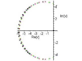
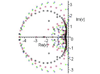
(((a)(a)	(((a)(b)
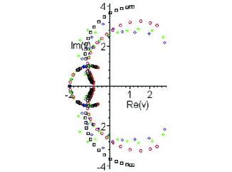
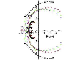
(((a)(c)	(((a)(d)

Figure 7: Partition-function zeros, in the $v$ plane, of (a) $Z(G,q,v)/q$ for $q=0$, and $Z(G,q,v)$ for (b) $q=0.999$, (c) $q=2$, and (d) $q=3$ on strips with free boundary conditions and several widths $L_{y}$: 2 ($\Box$, black), 3 ($\circ$, red), 4 ($+$, green), and 5 ($\Diamond$, blue), where the colors refer to the online paper.

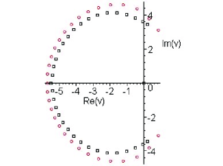
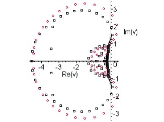
(((a)(a)	(((a)(b)
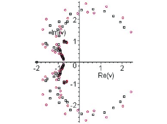
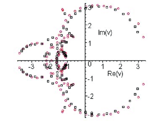
(((a)(c)	(((a)(d)

Figure 8: Partition-function zeros, in the $v$ plane, of (a) $Z(G,q,v)/q$ for $q=0$, and $Z(G,q,v)$ for (b) $q=0.999$, (c) $q=2$, and (d) $q=3$ on strips with cylindrical boundary conditions and several widths $L_{y}$: 4 ($\Box$, black), 6 ($\circ$, red), where the colors refer to the online paper.

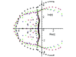
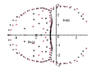
(((a)(a)	(((a)(b)

Figure 9: Partition-function zeros, in the $v$ plane for $q=q_{5}=(1/2)(3+\sqrt{5}\ )$ for (a) free boundary conditions with $L_{y}=$ 2 ($\Box$, black), 3 ($\circ$, red), 4 ($+$, green), and 5 ($\Diamond$, blue); (b) cylindrical boundary conditions and $L_{y}=$: 4 ($\Box$, black), 6 ($\circ$, red), where the colors refer to the online paper.

6.2 $q=0$

From the cluster representation of $Z(G,q,v)$, eq. (1.1), it follows that this partition function has an overall factor of $q^{k(G)}$, where $k(G)$ denotes the number of components of $G$, i.e., an overall factor of $q$ for a connected graph. Hence, $Z(G,q=0,v)=0$. In the transfer matrix formalism, this is evident from the overall factor of $q$ coming from the vector ${\bf w}$. However, if we first take the limit $n\to\infty$ to define ${\cal B}$ for $q\neq 0$ and then let $q\to 0$ or, equivalently, extract the factor $q$ from the left vector ${\bf w}$, we obtain a nontrivial locus, namely $({\cal B}_{v}(\{G\},0)_{qn}$. This is a consequence of the noncommutativity (6.2) for $q=0$.

With the second order of limits or the equivalent removal of the factor of $q$ in $Z$, we obtain the zeros for $q=0$ shown in Figures 7(a) (free boundary conditions) and 8(a) (cylindrical boundary conditions). The zeros appear to converge to a roughly circular curve. We see in these figures that the limiting curves cross the real $v$-axis at $v\approx-6$. As $L_{y}$ increases, the arc endpoints on the upper and lower right move toward the real axis. It is possible that these could pinch this axis at $v=0$ as $L_{y}\to\infty$, corresponding to the root of (6.3) for $q=0$.

6.3 $q=1$

For $q=1$, the spin-spin interaction in ${\cal H}$ always has the Kronecker delta function equal to unity, and hence the Potts model partition function is given by

$$Z(G,q=1,v)=e^{K|E|}=(1+v)^{|E|}$$ (6.10)

where $|E|$ is the number of edges in the graph $G$. This has a single zero at $v=-1$. But again, one encounters the noncommutativity (6.2) for $q=1$. It is interesting to analyze this in terms of the transfer matrix formalism. At this value of $q$, both the transfer matrix and the left vector ${\bf w}$ are non-trivial. There is thus a cancellation of terms that yields the result (6.10). The strip with $L_{y}=2$ and free boundary conditions is the simplest one to analyze: the eigenvalues and coefficients for $q=1$ are given by

$$\lambda_{1}(1,v)&=v^{4}\ ;\qquad\quad c_{1}(1,0)=0\\ \lambda_{2}(1,v)=(1+v)^{5}\ ;\quad c_{2}(1,0)=(1+v)$$ (6.11)

Thus, only the second eigenvalue contributes to the partition function, and it gives the expected result $Z(2\times m,FF,q=1,v)=(1+v)^{5m+1}$. The strip with $L_{y}=3$ and free boundary conditions is similar: there is a single eigenvalue $\lambda_{1}(1,v)=(1+v)^{8}$ with a non-zero coefficient $c_{1}(1,v)$ equal to $(1+v)$ for odd $L_{x}$ and $(1+v)^{5}$ for even $L_{x}$. The other four eigenvalues including $v^{4}(1+v)^{2}$ and the roots of

$$x^{3}-2v^{4}(v^{3}+6v^{2}+4v+1)x^{2}+v^{8}(1+v)^{2}(v^{4}+10v^{3}+15v^{2}+6v+1)x-v^{14}(1+v)^{6}=0$$ (6.12)

have identically zero coefficients. Thus, the partition function takes the form $Z(3\times m,FF,q=1,v)=(1+v)^{8m+k}=(1+v)^{|E|}$, where $k$=1 for odd $L_{x}$ and 5 for even $L_{x}$.

In general, we conclude that at $q=1$, only the eigenvalue $\lambda=(1+v)^{3L_{y}}$ contributes to the partition function for cylindrical boundary conditions, and only the eigenvalue $\lambda=(1+v)^{3L_{y}-1}$ contributes to the partition function for free b.c. The other eigenvalues do not contribute because they have zero coefficients in eq. (2.2). This is analogous to what we found in earlier work for cyclic strips [4, 5, 11].

In our present case, in order to get insight into ${\cal B}_{qn}$, we have computed the partition function zeros for a value of $q$ close to 1, namely, $q=0.999$ (see Figures 7(b) and 8(b)). The patterns of zeros show less scatter for cylindrical, as contrasted with free, boundary conditions. Subsituting $r=3$, i.e., $q=q_{3}=1$ in the solutions (6.6)-(6.8) of the criticality equation (6.3), we have

$$v_{hc1}=-4\cos(\pi/3)\cos(2\pi/9)=-1.5320888...$$ (6.13)

$$v_{hc2}=-4\cos(\pi/3)\cos(4\pi/9)=-0.34729635...$$ (6.14)

$$v_{hc3}=4\cos(\pi/3)\cos(\pi/9)=1.8793852...$$ (6.15)

Our results are consistent with the inference that as $L_{y}\to\infty$, the locus ${\cal B}_{v}$ crosses the real $v$ axis at the values of $v_{hc1}$ and $v_{hc2}$ in eqs. There is evidently no indication of any crossing near the value $v_{hc3}$. A noteworthy feature of the patterns of zeros, at least for the case of cylindrical boundary conditions, is that they do not appear to exhibit the prongs that tend to occur for some other cases discussed here.

6.4 $q=2$

The zeros for the $q=2$ Ising case are displayed in Figures 7(c) and 8(c) for free and cylindrical boundary conditions, respectively. (Fig. 7(c) extends our previous calculation presented in Fig. 3 of [1] to greater widths.) From our earlier work [4, 11] one knows that the loci ${\cal B}_{v}$ are different for strips with free or periodic transverse boundary conditions and free longitudinal boundary conditions, on the one hand, and free or periodic transverse boundary conditions and periodic (or twisted periodic) longitudinal boundary conditions. One anticipates, however, that in the limit of infinite width, the subset of the complex-temperature phase diagram that is relevant to real physical thermodynamics will be independent of the boundary conditions used to obtain the 2D thermodynamic limit.

In the 2D thermodynamic limit, one knows the complex-temperature phase diagram exactly for the $q=2$ (Ising) case. (This isomorphism involves the redefinition of the spin-spin exchange constant $J_{\rm Potts}=2J_{\rm Ising}$ and hence $K_{\rm Potts}=2K_{\rm Ising}$, where $K_{\rm Potts}$ is denoted simply $K$ here.) Since the honeycomb lattice is bipartite, the phase boundary separating the paramagnetic and ferromagnetic phases maps into that separating the paramagnetic and antiferromagnetic phases under the transformation $K\to-K$, i.e., $a\to 1/a$, where $a=e^{K}=v+1$. The total boundary locus ${\cal B}$ is invariant under this inversion $a\to 1/a$. Because of this symmetry, it is convenient to discuss the phase diagram first in terms of the variable $a$; the features in the $v$ plane then follow in an obvious manner. Following the calculation of the zero-field free energy $f$ of the Ising model on the square lattice [43], $f$ was calculated on the triangular and honeycomb lattices in [44]. The critical points separating the PM and FM phases are given by $a_{c}=2+\sqrt{3}$ and $1/a_{c}=2-\sqrt{3}$, respectively. In terms of $v$, these correspond to the values $v_{hc3}$ and $v_{hc2}$ with $r=4$ in eqs. (6.8) and (6.7). The complex-temperature phase diagram, with boundaries comprised by the locus ${\cal B}$, was given in the plane of the variable ${\rm tanh}(K)=(a-1)/(a+1)$ in (Fig. 3 of) [45] and in the variable $a$ in (Fig. 1(c) of) [46]. The locus ${\cal B}$ separates the complex $a$ plane into three phases: (i) the physical PM phase occupying the interval $2-\sqrt{3}\leq a\leq 2+\sqrt{3}$, and its complex-temperature extension (CTE), where the $S_{q}$ symmetry is realized explicitly ($S_{q}$ being the symmetric group on $q$ numbers, the symmetry group of the Hamiltonian), (ii) the physical ferromagnetic phase occupying the interval $2+\sqrt{3}\leq a\leq\infty$ (and its CTE), and (iii) the physical antiferromagnetic phase occupying the interval $0\leq a\leq 2-\sqrt{3}$ and its CTE. The boundary separating the CTE of the FM and AFM phases is an arc of the unit circle $a=e^{i\theta}$ with $\pi/3\leq\theta\leq 5\pi/3$; it thus has endpoints at $a=e^{\pm i\pi/3}$ and crosses the real $a$ axis at $a=-1$. The rest of ${\cal B}$ is a closed curve crossing the real axis at $a=2\pm\sqrt{3}$ and having intersection points with the above-mentioned circular arc at the points at $a=\pm i$. In [1] the locus ${\cal B}$ for an infinite-length free and cyclic strip with width $L_{y}=2$ were compared with this 2D phase diagram.

Using our exact results, we can compare the loci ${\cal B}_{v}$ for various strip widths and either free or periodic transverse boundary conditions with the known complex-temperature phase diagram for the Ising model on the infinite 2D honeycomb lattice. This comparison is simplest for the case of free boundary conditions, so we concentrate on these results. For the finite values of $L_{y}$ that we have considered, the loci ${\cal B}_{v}$ inferred from these zeros clearly contain a circular arc crossing the real $v$ axis at $v=-2$ and have intersection points at $v=-1\pm i$, just as is the case with the exactly known locus ${\cal B}$ for the infinite 2D honeycomb lattice. Moreover, one sees that as $L_{y}$ increases, the endpoints of the complex-conjugate arcs move down toward the real axis. As $L_{y}\to\infty$, we expect that these arc endpoints will cross the real $v$ axis at the points $v=1\pm\sqrt{3}$ that constitute the intersections, with the real $v$ axis, of the complex-temperature phase boundaries ${\cal B}$ for the Ising model on the infinite honeycomb lattice. As in our earlier studies, this comparison shows that, although the behavior of the asymptotic locus ${\cal B}$ for infinite-length lattice strips is qualitatively different from the locus for the thermodynamic limit of the two-dimensional lattice as regards the physical phase transitions (owing to its quasi-one-dimensional nature), its features for complex temperatures show many similarities with the exactly known features for the 2D thermodynamic limit.

6.5 $q=(3+\sqrt{5})/2$

One of the useful features of exact solutions for $Z(G,q,v)$ for arbitrary $q$ and $v$ is that they allow one to analyze values of $q$ that are not positive integers and hence cannot be represented in Hamiltonian form, but instead via the relation (1.1). Within the sequence of the $q_{r}$’s, the first such example is provided by the case $r=5$, i.e., $q=q_{5}=(3+\sqrt{5})/2\simeq 2.6180$. For this value, the criticality condition for the model on the (thermodynamic limit of the) honeycomb lattice has the solutions

$$v_{hc3}=\frac{1}{2}\Big{[}1+\sqrt{3(5+2\sqrt{5})\ }\ \Big{]}\simeq 3.165$$ (6.16)

$$v_{hc2}=-1$$ (6.17)

$$v_{hc1}=\frac{1}{2}\Big{[}1-\sqrt{3(5+2\sqrt{5})\ }\ \Big{]}\simeq-2.165$$ (6.18)

The first of these is the PM-FM critical point, while the second formally corresponds to the critical temperature for the Potts antiferromagnet going to zero. The third is a complex-temperature singular point. In Figs. 9 we plot zeros of the partition function in the $v$ plane for $q=q_{5}$ and strips with free and cylindrical boundary conditions. From these zeros, one can infer that as $L_{y}\to\infty$, the rightmost complex-conjugate arc endpoints would move in and pinch the real axis at the PM-FM value $v_{hc3}\simeq 3.165$ given in eq. (6.16). The results are also consistent with crossings on ${\cal B}$ at the other two points $v_{hc2}$ and $v_{hc1}$ as well as the values $v\simeq-0.6$ and $v\simeq-4.4$ which are not roots of the criticality condition (6.3).

6.6 $q=3$

In contrast to the $q=2$ case, the free energy of the $q$-state Potts model has not been calculated exactly for $q\geq 3$ on any 2D (or higher-dimensional) lattice, and hence the corresponding complex-temperature phase diagrams are not known exactly. For $q=3$, i.e., $r=6$, the solutions of the criticality equation (6.3) given by eqs. (6.6)-(6.8) are

$$v_{hc3}=2\sqrt{3}\cos(\pi/18)=3.4114741...$$ (6.19)

corresponding to the physical PM-FM phase transition point, and two other roots at the complex-temperature values

$$v_{hc2}=-2\sqrt{3}\cos(7\pi/18)=-1.1847925...$$ (6.20)

and

$$v_{hc1}=-2\sqrt{3}\cos(5\pi/18)=-2.2266815...$$ (6.21)

Some discussions of the complex-temperature solutions of eq. (6.3) and their connections with the complex-temperature phase diagram have been given in [47]-[49].

The partition-function zeros in the $v$ plane for $q=3$ are displayed in Figures 7(d) and 8(d) for free and cylindrical boundary conditions, respectively. We expect that the pair of complex-conjugate endpoints in this regime will eventually converge to the ferromagnetic critical point $v_{hc3}$ as $L_{y}\to\infty$. However, obviously, an infinite-length strip of finite width $L_{y}$ is a quasi-one-dimensional system, so the Potts model has no physical finite-temperature phase transition on such a strip for any finite $L_{y}$. The $q=3$ Potts antiferromagnet is disordered on the honeycomb lattice for all temperatures $T$ including $T=0$, so there is no finite-temperature PM-AFM transition.

In the complex-temperature interval $v<-1$, there are considerable finite-size and boundary condition effects. Because of this, in previous work, a combination of partition-function zeros and analyses of low-temperature series expansions was used [49]; these enable one at least to locate some points on the complex-temperature phase boundary. As regards the infinite 2D honeycomb lattice, because of a duality relation, the complete physical temperature interval $0\leq T\leq\infty$, i.e., $0\leq a\leq 1$ of the $q$-state Potts antiferromagnet on the triangular lattice is mapped to the complex-temperature interval $-\infty\leq v\leq-q)$ on the honeycomb lattice (and vice versa) [48]. Ref. [48] found that there is a complex-temperature singularity for the $q=3$ Potts model at $v_{tri,PM-AFM,q=3}=-0.79691\pm 0.00003$. From duality, the corresponding singularity on the honeycomb lattice is $v_{hc,q=3}=3/v_{tri,PM-AFM,q=3}=-3.76454\pm 0.00015$. One anticipates that as $L_{y}\to\infty$ for the infinite-length, width-$L_{y}$ strips of the honeycomb lattice, the left-most arcs on ${\cal B}_{v}$ will cross the real $v$ axis at this point. There are several other cases of interest, such as $q=4$ and $q_{r}$ values with $r\geq 7$. For brevity, we do not consider these here.

7 Internal Energy and Specific Heat

It is of interest to display some of the physical thermodynamic functions for the Potts model on the infinite-length limits of these strips. Having calculated the partition function, one obtains the free energy per site, $f(G,q,v)$ as

$$f(G,q,v)={1\over n}\log Z(G,q,v)$$ (7.1)

for finite $n$, with the $n\to\infty$ limit having been defined in eq. (1.2) above. The internal energy per site, $E$, is

$$E(G,q,v)=-\frac{\partial f}{\partial\beta}=-J(v+1)\frac{\partial f}{\partial v}{}$$ (7.2)

and the specific heat per site, $C$, is

$$C=\frac{\partial E}{\partial T}=k_{B}K^{2}(v+1)\left[\frac{\partial f}{\partial v}+(v+1)\frac{\partial^{2}f}{\partial v^{2}}\right]\ .$$ (7.3)

As the strip width $L_{y}\to\infty$, these approach the internal energy and specific heat for the infinite 2D honeycomb lattice. For convenience we define a dimensionless internal energy

$$E_{r}=-\frac{E}{J}=(v+1)\frac{\partial f}{\partial v}\ .$$ (7.4)

Note that $\mathop{\rm sgn}\nolimits(E_{r})$ is (i) opposite to $\mathop{\rm sgn}\nolimits(E)$ in the ferromagnetic case where $J>0$ for which the physical region is $0\leq v\leq\infty$ and (ii) the same as $\mathop{\rm sgn}\nolimits(E)$ in the antiferromagnet case $J<0$ for which the physical region is $-1\leq v\leq 0$. Of course, the infinite-length limits of the honeycomb-strips considered here are quasi-one-dimensional systems, so that $f$, $E$, and $C$ are analytic functions of temperature for all finite temperatures.

We recall the high-temperature (equivalently, small–$|K|$) expansion for an infinite lattice of dimensionality $d\geq 2$ with coordination number $\Delta$:

$$-\frac{E}{J}=E_{r}=\frac{\Delta}{2}\left[\frac{1}{q}+\frac{(q-1)K}{q^{2}}+O(K^{3})\right]\ .$$ (7.5)

Here, $\Delta=3$ for the infinite honeycomb lattice. Again, we recall that in papers on the $q=2$ Ising special case, the Hamiltonian is usually defined as ${\cal H}_{I}=-J_{I}\sum_{\langle ij\rangle}\sigma_{i}\sigma_{j}$ with $\sigma_{i}=\pm 1$ rather than the Potts model definition of ${\cal H}$, so that one has the rescaling $2K_{I}=K$, where $K_{I}=\beta J_{I}$. Furthermore, $E_{I}=-J\langle\sigma_{i}\sigma_{j}\rangle$ raher than the Potts definition $E=-J\langle\delta_{\sigma_{i}\sigma_{j}}\rangle$, where $\langle ij\rangle$ are adjacent vertices. Hence, for example, for $q=2$, with the usual Ising model definitions, $E_{I}(v=0)=0$ rather than $E=-J\Delta/(2q)$ and the high-temperature expansion is $E_{I}=-J(\Delta/2)[K+O(K^{3})]$ rather than the $q=2$ form of (7.5). Similarly, for $T\to 0$, with the conventional Ising definition, $E_{I}\to-|J|$ for both the ferromagnetic and antiferromagnetic cases, while with our Potts-based definition, $E\to-(\Delta/2)J=-3J/2$, i.e., $E_{r}\to 3/2$ for the ferromagnet and $E\to 0$ for the antiferromagnet.

We next present plots of the the (reduced) internal energy $E_{r}$ per site and the specific heat per site $C$ on infinite-length honeycomb-lattice strips for three values of $q$ in increasing order, $q=2$, $q=(3+\sqrt{5})/2$, and $q=3$ in the respective Figs. 10-12. Each plot contains curves for $L_{y}$ from 2 to 5 for strips with free boundary conditions and for $L_{y}=4$ and $L_{y}=6$ for strips with cylindrical boundary conditions. The free energy and its derivatives with respect to the temperature are independent of the longitudinal boundary conditions in the limit $L_{x}\to\infty$, although they depend on the transverse boundary conditions [4]. As expected, in the vicinity of the infinite-temperature point $v=0$, the results for the internal energy are well described by the first few terms of the high-temperature series expansion given in eq. (7.5). One can see the approach of $E_{r}$ to its zero-temperature limit of 1.5 for the ferromagnet as $v$ increases through positive values. This approach is more rapid for the strips with cylindrical boundary conditions, as is understandable since these minimize finite-size effects in the transverse direction. One can also see the approach of $E_{r}$ to its zero-temperature limit of zero for the antiferromagnet as $v$ decreases toward $v=-1$.

With regard to the specific heat, the plots show maxima which occur at values of $v$, denoted $v_{m}$, that depend on the values of $q$ and $L_{y}$ and the transverse boundary conditions. In the ferromagnetic case, these approach the critical values for the infinite honeycomb lattice, $v_{PM-FM}$, as $L_{y}$ increases. For the results shown, this approach is from above (below) in $v$ for the case of free (cylindrical) boundary conditions. The heights of the maxima increase as $L_{y}$ increases, in accordance with the fact that on 2D lattices, the specific heat diverges at the PM-FM critical point for the values of $q$ shown. (This divergence is logarithmic for $q=2$ [43]; more generally, for the interval $0\leq q\leq 4$ where the 2D Potts ferromagnet has a second-order transition, the specific heat exponent is given by $\alpha=\alpha^{\prime}=(2/3)(\pi-2\theta)/(\pi-\theta)$ [33, 34], where $\theta=2\,{\rm arccos}(q^{1/2}/2)$ as in eq. (6.4), so $\alpha=2/9$ for $q=(3+\sqrt{5})/2$ and $\alpha=1/3$ for $q=3$.) This behavior as a function of increasing strip width $L_{y}$ is the analogue, for these infinite-length strips, of the standard finite-size scaling behavior of the specific heat on $L\times L$ sections of a regular lattice, for which $|v_{m}-v_{PM-FM}|\sim L^{-1/\nu}$ and $C(v=v_{m})\sim L^{\alpha/\nu}$, where $\nu=\nu^{\prime}$ is the correlation length critical exponent [50, 51] for the Potts ferromagnet on a two-dimensional lattice, with $\nu$ being related to $\alpha$ by the hyperscaling relation $d\nu=2-\alpha$, so that $\nu=1$ for $q=2$ and $\nu=5/6$ for $q=3$. Note that $\alpha<0$ for $0<q<2$, so that, although the Potts ferromagnet has a PM-FM critical point for this range of $q$, with a divergent correlation length, the specific heat has only a finite, rather than divergent, nonanalyticity at the critical point.

We next consider the plots of the specific heat in the case of the Potts antiferromagnet. For $q=2$, $C$ exhibits a maximum at a value of $v$ that approaches the value $v_{PM-AFM}=1-\sqrt{3}$ for the 2D lattice as $L_{y}$ increases, and the height of the maximum increases; these are simply related, by $K\to-K$, to the behavior for the $q=2$ ferromagnet. For $q=(3+\sqrt{5})/2$ the curves for the specific heat in the antiferromagnetic region of Fig. 11 exhibit a maximum not too far from the zero-temperature value $v=-1$. However, the height of the maximum does not increase very much as $L_{y}$ increases, for either the free or cylindrical boundary conditions. Finally, we show $E_{r}$ and $C$ for $q=3$, in Fig. 12. For this value of $q$ the Potts antiferromagnet has no finite-temperature PM-AFM transition and is noncritical even at $T=0$; consistent with this, although $C$ has a maximum, the height of this maximum does not increase with increasing $L_{y}$.

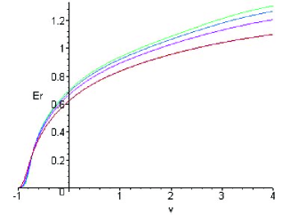
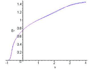
(((a)(a)	(((a)(b)
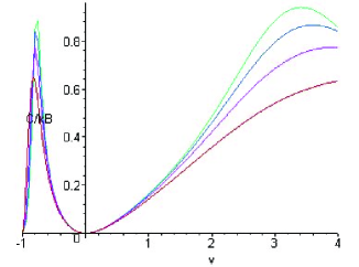
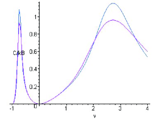
(((a)(c)	(((a)(d)

Figure 10: Reduced internal energy $E_{r}=-E/J$ and specific heat $C/k_{B}$ as functions of the temperature-like variable $v$ for the $q=2$ Potts model on the honeycomb-lattice strips of width $2\leq L_{y}\leq 5$ with free boundary conditions (a) (c) and of width $L_{y}=4,6$ with cylindrical boundary conditions (b) (d). The four curves shown for the case of free boundary conditions correspond to $L_{y}=2,3,4,5$ as one moves upward and the two curves for cylindrical boundary conditions correspond to $L_{y}=4,6$ as one moves upward. The plot includes both the ferromagnetic and antiferromagnetic Potts models, for which the temperature ranges are $0\leq v\leq\infty$ and $-1\leq v\leq 0$, respectively.

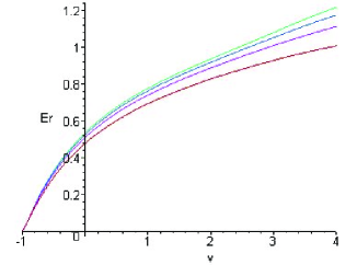
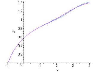
(((a)(a)	(((a)(b)
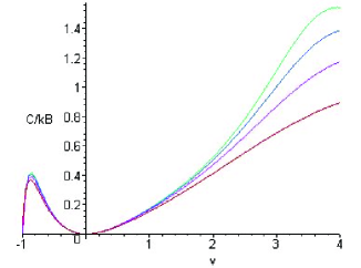
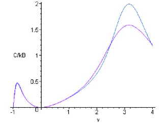
(((a)(c)	(((a)(d)

Figure 11: Reduced internal energy $E_{r}=-E/J$ and specific heat $C/k_{B}$ as functions of the temperature-like variable $v$ for the Potts model with $q=(3+\sqrt{5})/2$ on the honeycomb-lattice strips of width $2\leq L_{y}\leq 5$ with free boundary conditions (a) (c) and of width $L_{y}=4,6$ with cylindrical boundary conditions (b) (d). Ordering of curves is as in Fig. 10.

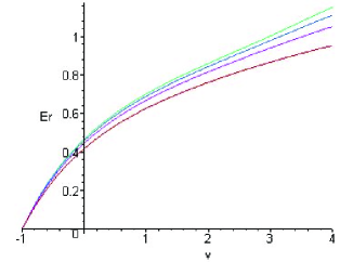
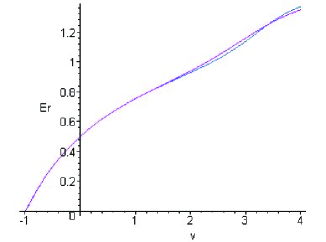
(((a)(a)	(((a)(b)
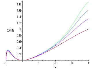
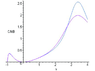
(((a)(c)	(((a)(d)

Figure 12: Reduced internal energy $E_{r}=-E/J$ and specific heat $C/k_{B}$ as functions of the temperature-like variable $v$ for the $q=3$ Potts model on the honeycomb-lattice strips of width $2\leq L_{y}\leq 5$ with free boundary conditions (a) (c) and of width $L_{y}=4,6$ with cylindrical boundary conditions (b) (d). Ordering of curves is as in Fig. 10.

Acknowledgment

This research was partially supported by the Taiwan NSC grant NSC-95-2112-M-006-004 and NSC-95-2119-M-002-001 (S.-C.C.) and the U.S. NSF grant PHY-03-54776 (R.S.).

8 Appendix: Transfer Matrix for $L_{y}=4$ Strip with Cylindrical Boundary Conditions

The number of elements in the basis is eight: ${\bf P}=\{\delta_{1,2,3,4},\delta_{1,2,3}+\delta_{1,2,4}+\delta_{1,3,4}+\delta_{2,3,4},\delta_{1,2}\delta_{3,4},\delta_{1,2}+\delta_{3,4},\delta_{1,3}+\delta_{2,4},\delta_{1,4}\delta_{2,3},\delta_{2,3}+\delta_{1,4},1\}$. The transfer matrix is given by

$${\mathsf{T}}=$$ (8.1)

$$\left(\begin{array}[]{cccccccc}v^{8}D_{1}^{2}D_{3}^{2}&4v^{8}D_{1}D_{3}S_{25}&v^{8}D_{1}^{2}T_{13}&2v^{8}D_{1}T_{14}&2v^{8}S_{25}^{2}&v^{9}D_{2}D_{3}^{2}&2v^{9}D_{3}S_{23}&v^{9}T_{18}\\ v^{6}D_{1}^{2}D_{3}S_{25}&v^{6}D_{1}T_{22}&v^{6}D_{1}^{2}T_{23}&v^{6}D_{1}T_{24}&v^{6}S_{25}T_{25}&v^{7}D_{2}D_{3}S_{25}&v^{7}T_{27}&v^{7}T_{28}\\ 0&0&v^{8}D_{1}^{2}&2v^{9}D_{1}&0&0&0&v^{10}\\ v^{4}D_{1}^{2}S_{25}^{2}&2v^{4}D_{1}S_{25}T_{25}&v^{4}D_{1}^{2}T_{43}&v^{4}D_{1}T_{44}&2v^{5}S_{23}S_{33}&v^{5}D_{2}S_{25}^{2}&2v^{5}S_{25}T_{47}&v^{5}T_{48}\\ v^{4}D_{1}^{2}S_{25}^{2}&2v^{4}D_{1}S_{25}T_{25}&v^{5}D_{1}^{2}T_{53}&2v^{5}D_{1}T_{54}&v^{4}T_{55}&v^{5}D_{2}S_{25}^{2}&2v^{5}S_{25}T_{47}&v^{6}T_{58}\\ v^{6}D_{1}^{2}T_{61}&4v^{6}D_{1}T_{62}&v^{6}D_{1}^{2}F_{2}^{2}&2v^{6}D_{1}F_{2}S_{42}&2v^{6}F_{2}T_{65}&v^{6}T_{66}&2v^{6}T_{67}&v^{6}S_{42}^{2}\\ v^{3}D_{1}^{2}T_{71}&2v^{3}D_{1}T_{72}&v^{3}D_{1}^{2}T_{73}&2v^{3}D_{1}T_{74}&2v^{3}T_{75}&v^{3}T_{76}&v^{3}T_{77}&v^{3}T_{78}\\ D_{1}^{2}T_{23}T_{81}&4D_{1}T_{82}&D_{1}^{2}T_{83}&2D_{1}T_{84}&2T_{85}T_{85}^{\prime}&T_{86}&T_{87}&T_{88}\end{array}\right)$$ (8.10)

where the factors $D_{k}$ and $F_{k}$ are defined in eqs. (LABEL:def_Dk) and (LABEL:def_Fk); the $T_{ij}$ are given by

$$T_{13}&=2q+6v+v^{2}\\ T_{14}=q^{2}+4qv+7v^{2}+v^{3}\\ T_{15}=q+8v+4v^{2}\\ T_{18}=2q^{2}+6qv+8v^{2}+v^{3}$$ (8.12)

$$T_{22}&=5q^{2}+q^{2}v+34qv+10qv^{2}+65v^{2}+33v^{3}+4v^{4}\\ T_{23}=q^{2}+5qv+8v^{2}+v^{3}\\ T_{24}=q^{3}+7q^{2}v+17qv^{2}+19v^{3}+2v^{4}\\ T_{25}=q^{2}+6qv+11v^{2}+2v^{3}\\ T_{27}=5q^{2}+q^{2}v+28qv+8qv^{2}+41v^{2}+19v^{3}+2v^{4}\\ T_{28}=q^{3}+6q^{2}v+12qv^{2}+11v^{3}+v^{4}$$ (8.13)

$$T_{43}&=q^{3}+6q^{2}v+14qv^{2}+14v^{3}+v^{4}\\ T_{44}=q^{4}+8q^{3}v+26q^{2}v^{2}+42qv^{3}+33v^{4}+2v^{5}\\ T_{47}=q^{2}+5qv+7v^{2}+v^{3}\\ T_{48}=q^{4}+7q^{3}v+20q^{2}v^{2}+28qv^{3}+19v^{4}+v^{5}$$ (8.14)

$$T_{53}&=2q^{2}+8qv+10v^{2}+v^{3}\\ T_{54}=q^{3}+6q^{2}v+13qv^{2}+12v^{3}+v^{4}\\ T_{55}=q^{4}+8q^{3}v+32q^{2}v^{2}+2q^{2}v^{3}+68qv^{3}+12qv^{4}+61v^{4}+22v^{5}+2v^{6}\\ T_{58}=2q^{3}+10q^{2}v+18qv^{2}+14v^{3}+v^{4}$$ (8.15)

$$T_{61}&=q+6v+2v^{2}\\ T_{62}=q^{2}+6qv+qv^{2}+10v^{2}+3v^{3}\\ T_{65}=q^{2}+4qv+8v^{2}+2v^{3}\\ T_{66}=q^{2}+8qv+3qv^{2}+21v^{2}+16v^{3}+3v^{4}\\ T_{67}=q^{3}+7q^{2}v+q^{2}v^{2}+18qv^{2}+4qv^{3}+17v^{3}+5v^{4}$$ (8.16)

$$T_{71}&=q^{3}+8q^{2}v+q^{2}v^{2}+25qv^{2}+6qv^{3}+32v^{3}+13v^{4}+v^{5}\\ T_{72}=2q^{4}+17q^{3}v+q^{3}v^{2}+62q^{2}v^{2}+8q^{2}v^{3}+117qv^{3}+25qv^{4}+98v^{4}+34v^{5}+2v^{6}\cr\\ T_{73}=q^{4}+7q^{3}v+21q^{2}v^{2}+32qv^{3}+22v^{4}+v^{5}\\ T_{74}=q^{5}+8q^{4}v+28q^{3}v^{2}+54q^{2}v^{3}+58qv^{4}+30v^{5}+v^{6}\\ T_{75}=q^{5}+9q^{4}v+37q^{3}v^{2}+q^{3}v^{3}+87q^{2}v^{3}+7q^{2}v^{4}+118v^{4}q+19v^{5}q+74v^{5}+21v^{6}\cr+v^{7}\\ T_{76}=q^{4}+10vq^{3}+2v^{2}q^{3}+41v^{2}q^{2}+16v^{3}q^{2}+v^{4}q^{2}+88v^{3}q+52v^{4}q+7qv^{5}+88v^{4}\cr+72v^{5}+17v^{6}+v^{7}\\ T_{77}=2q^{5}+19q^{4}v+q^{4}v^{2}+78q^{3}v^{2}+8q^{3}v^{3}+180q^{2}v^{3}+28q^{2}v^{4}+240qv^{4}+52qv^{5}\cr+149v^{5}+47v^{6}+2v^{7}\\ T_{78}=q^{6}+9vq^{5}+36q^{4}v^{2}+83q^{3}v^{3}+118q^{2}v^{4}+99qv^{5}+41v^{6}+v^{7}$$ (8.17)

$$T_{81}&=q^{3}+5q^{2}v+12qv^{2}+qv^{3}+16v^{3}+4v^{4}\\ T_{82}=q^{6}+11q^{5}v+55q^{4}v^{2}+q^{4}v^{3}+162q^{3}v^{3}+9q^{3}v^{4}+302q^{2}v^{4}+34q^{2}v^{5}+345qv^{5}\cr+67qv^{6}+qv^{7}+192v^{6}+61v^{7}+4v^{8}\\ T_{83}=q^{6}+10q^{5}v+45q^{4}v^{2}+118q^{3}v^{3}+194q^{2}v^{4}+194qv^{5}+qv^{6}+96v^{6}+4v^{7}\\ T_{84}=q^{7}+11q^{6}v+55q^{5}v^{2}+163q^{4}v^{3}+313q^{3}v^{4}+396q^{2}v^{5}+313qv^{6}+qv^{7}+126v^{7}\cr+4v^{8}\\ T_{85}=q^{3}+6q^{2}v+14qv^{2}+13v^{3}+v^{4}\\ T_{85}^{\prime}=q^{4}+6q^{3}v+16q^{2}v^{2}+25qv^{3}+qv^{4}+22v^{4}+4v^{5}\\ T_{86}=q^{6}+12q^{5}v+q^{5}v^{2}+65q^{4}v^{2}+12q^{4}v^{3}+206q^{3}v^{3}+63q^{3}v^{4}+2q^{3}v^{5}+412q^{2}v^{4}\cr+184q^{2}v^{5}+15q^{2}v^{6}+512qv^{5}+312qv^{6}+46qv^{7}+qv^{8}+320v^{6}+256v^{7}\cr+60v^{8}+4v^{9}\\ T_{87}=2q^{7}+24q^{6}v+132q^{5}v^{2}+2v^{3}q^{5}+434q^{4}v^{3}+18q^{4}v^{4}+934q^{3}v^{4}+72q^{3}v^{5}\cr+1346q^{2}v^{5}+166q^{2}v^{6}+1232qv^{6}+230qv^{7}+2qv^{8}+560v^{7}+160v^{8}+8v^{9}\cr\\ T_{88}=q^{8}+12q^{7}v+66q^{6}v^{2}+218q^{5}v^{3}+477q^{4}v^{4}+718q^{3}v^{5}+739q^{2}v^{6}+486qv^{7}\cr+qv^{8}+165v^{8}+4v^{9}$$ (8.18)

The vectors ${\bf w}$ and ${\bf u}_{\rm id}$ are given by

$${\bf w}_{\rm odd}^{\rm T}&=q\left(D_{1}^{2},4D_{1}F_{1},qD_{1}^{2},2qD_{1}F_{1},2F_{1}^{2},q+2v+v^{2},2F_{1}^{2},qF_{1}^{2}\right)\\ {\bf w}_{\rm even}^{\rm T}=q\left(D_{1}^{2}X_{2}^{2},4D_{1}X_{1}X_{2},D_{1}^{2}X_{3},2D_{1}X_{4},2X_{1}^{2},(q+2v+v^{2})X_{2}^{2},2X_{2}X_{5},X_{6}\right)\cr\\ {\bf u}_{\rm id}^{\rm T}=\left(1,0,0,0,0,0,0,0\right)$$ (8.19)

where

$$X_{3}&=v^{6}+6v^{5}+15v^{4}q+20v^{3}q^{2}+15v^{2}q^{3}+6q^{4}v+q^{5}\\ X_{4}=v^{7}+7v^{6}+21v^{5}q+35v^{4}q^{2}+35q^{3}v^{3}+21q^{4}v^{2}+7vq^{5}+q^{6}\\ X_{5}=v^{5}+5v^{4}+10v^{3}q+10v^{2}q^{2}+5vq^{3}+q^{4}\\ X_{6}=v^{8}+8v^{7}+28v^{6}q+56v^{5}q^{2}+70q^{3}v^{4}+56q^{4}v^{3}+28v^{2}q^{5}+8q^{6}v+q^{7}\cr$$ (8.20)

References

- [1] S.-C. Chang and R. Shrock, Physica A 296, 183 (2001).
- [2] C. M. Fortuin and P. W. Kasteleyn, Physica 57, 536 (1972).
- [3] H. W. J. Blöte and M. P. Nightingale, Physica A 112, 405 (1982).
- [4] R. Shrock, Physica A 283, 388 (2000).
- [5] S.-C. Chang and R. Shrock, Physica A 296, 234 (2001).
- [6] S.-C. Chang and R. Shrock, Physica A 316, 335 (2002).
- [7] S.-C. Chang, J. Salas, and R. Shrock, J. Stat. Phys. 107, 1207 (2002).
- [8] S.-C. Chang and R. Shrock, Physica A 347, 314 (2005).
- [9] S.-C. Chang and R. Shrock, Physica A 364, 231 (2006).
- [10] J. L. Jacobsen, J.-F. Richard, and J. Salas, Nucl. Phys. B 743, 153 (2006); J. L. Jacobsen, private communication.
- [11] S.-C. Chang and R. Shrock, Physica A 286, 189 (2001).
- [12] S.-C. Chang, J. Jacobsen, J. Salas, and R. Shrock, J. Stat. Phys. 114, 763 (2004).
- [13] M. E. Fisher, in Lectures in Theoretical Physics (Univ. of Colorado Press, Boulder, CO, 1965), vol. 7C, p. 1.
- [14] R. Abe, Prog. Theor. Phys. 38, 322 (1967); S. Katsura, Prog. Theor. Phys. 38, 1415 (1967); S. Ono, Y. Karaki, M. Suzuki, and C. Kawabata, J. Phys. Soc. Jpn. 25, 54 (1968); H. Brascamp and H. Kunz, J. Math. Phys. 15, 65 (1974).
- [15] H. Klüpfel, Master’s Thesis, SUNY Stony Brook, May, 1999; H. Klüpfel and R. Shrock, unpublished.
- [16] S.-Y. Kim and R. Creswick, Phys. Rev. E 63, 066107 (2001).
- [17] N. J. A. Sloane, The On-Line Encyclopedia of Integer Sequences, http://www.research.att.com/ njas/sequences.
- [18] R. Donaghey, and L. Shapiro, J. Combin. Th. Ser. A 23, 291 (1977).
- [19] J. Salas and A. Sokal, J. Stat. Phys., 104, 609 (2001).
- [20] S.-C. Chang and R. Shrock, Physica A 296, 131 (2001).
- [21] R. Shrock and S.-H. Tsai, Physica A 259, 315 (1998).
- [22] S.-C. Chang and R. Shrock, J. Stat. Phys. 112, 815 (2003).
- [23] R. J. Baxter, J. Phys. A 20, 5241 (1987).
- [24] M. Roček, R. Shrock, and S.-H. Tsai, Physica A 252, 505 (1998).
- [25] R. Shrock and S.-H. Tsai, J. Phys. A 32 (Lett.), L195 (1999).
- [26] S.-C. Chang and R. Shrock, Physica A 346, 400 (2005).
- [27] R. Shrock and S.-H. Tsai, Phys. Rev. E60, 3512 (1999); Physica A 275, 429 (2000).
- [28] R. Shrock, Phys. Lett. A 261, 57 (1999).
- [29] R. Shrock, in the Proceedings of the 1999 British Combinatorial Conference, BCC99 (July, 1999), Discrete Math. 231, 421 (2001).
- [30] A. D. Sokal, Combin., Prob.. and Comput. 10, 41 (2001).
- [31] D. Kim and R. Joseph, J. Phys. C 7 (1974) L167.
- [32] T. W. Burkhardt and B. W. Southern, J. Phys. A 11 (1978) L247.
- [33] F. Y. Wu, Rev. Mod. Phys. 54, 235 (1982).
- [34] R. J. Baxter, Exactly Solved Models in Statistical Mechanics (Academic, London, 1982).
- [35] H. Feldmann, R. Shrock, and S.-H. Tsai, Phys. Rev. E 57, 1335 (1998).
- [36] R. Shrock and S.-H. Tsai, J. Math. Phys. A 30, 495 (1997).
- [37] J. Salas and A. D. Sokal, J.Stat. Phys. 86, 551 (1997).
- [38] W. T. Tutte, J. Combin. Theory 9, 289 (1970).
- [39] S. Beraha, J. Kahane, and N. Weiss, J. Combin. Theory B 27, 1 (1979); ibid. 28, 52 (1980).
- [40] P. P. Martin, Potts Models and Related Problems in Statistical Mechanics (World Scientific, Singapore, 1991).
- [41] H. Saleur, Commun. Math. Phys. 132, 657 (1990); Nucl. Phys. B 360, 219 (1991).
- [42] S.-C. Chang and R. Shrock, J. Phys. A 39, 10277 (2006).
- [43] L. Onsager, Phys. Rev. 65, 117 (1944).
- [44] R. Houtappel, Physica 16, 425 (1950); K. Husimi and I. Syozi, Prog. Theor. Phys. 5, 177 (1950); I. Syozi, Prog. Theor. Phys. 5, 341 (1950); G. Newell, Phys. Rev. 79, 876 (1950).
- [45] R. Abe, T. Dotera, and T. Ogawa, Prog. Theor. Phys. 85, 509 (1991).
- [46] V. Matveev and R. Shrock, J. Phys. A 29, 803 (1996).
- [47] P. P. Martin and J.-M. Maillard, J. Phys. A 19, L547 (1986).
- [48] H. Feldmann, R. Shrock, and S.-H. Tsai, J. Phys. A (Lett.) 30, L663 (1997).
- [49] H. Feldmann, A. J. Guttmann, I. Jensen, R. Shrock, and S.-H. Tsai, J. Phys. A 31, 2287 (1998).
- [50] M. Barber, in C. Domb and J. Lebowitz, eds., Phase Transitions and Critical Phenomena (Academic, New York, 1983), vol. 8, p. 146
- [51] J. L. Cardy, J. Phys. A 17, L385, L961 (1984); H. W. J. Blöte, and M. P. Nightingale, Phys. Rev. Lett. 56, 742 (1986); I. Affleck, Phys. Rev. Lett. 56, 746 (1986).