Spin dynamics across the superfluid-insulator
transition of spinful bosons

Abstract

Bosons with non-zero spin exhibit a rich variety of superfluid and insulating phases. Most phases support coherent spin oscillations, which have been the focus of numerous recent experiments. These spin oscillations are Rabi oscillations between discrete levels deep in the insulator, while deep in the superfluid they can be oscillations in the orientation of a spinful condensate. We describe the evolution of spin oscillations across the superfluid-insulator quantum phase transition. For transitions with an order parameter carrying spin, the damping of such oscillations is determined by the scaling dimension of the composite spin operator. For transitions with a spinless order parameter and gapped spin excitations, we demonstrate that the damping is determined by an associated quantum impurity problem of a localized spin excitation interacting with the bulk critical modes. We present a renormalization group analysis of the quantum impurity problem, and discuss the relationship of our results to experiments on ultracold atoms in optical lattices.

I Introduction

An important frontier opened by the study of ultracold atoms has been the investigation of Bose-Einstein condensates of atoms carrying a nonzero total spin $F$. The condensate wavefunction then has rich possibilities for interesting structure in spin space, analogous to structure investigated earlier in superfluid ³He. The dynamics of the atomic condensate is described by a multi-component Gross-Pitaevski (GP) equation, and this allows for interesting oscillations in the orientation of the condensate in spin space. Such coherent spin oscillations have been observed in a number of recent studies of $F=1$ and $F=2$ condensates ketterle1 ; chapman1 ; kurn ; chapman2 ; sengstock1 ; sengstock2 .

Coherent spin oscillations of a rather different nature are observed in the presence of a strong optical lattice potential bloch1 ; bloch2 . Here there is no Bose-Einstein condensate and the ground state is a Mott insulator: each minimum of the optical lattice potential traps a fixed number of atoms, and tunneling between neighboring potential minima can be ignored. Now the spin quantum number leads to a number of discrete atomic levels associated with each minimum, with the energies determined by the “cold collisional” interactions between the atoms. The coherent spin oscillations are then the Rabi oscillations between these atomic levels bloch1 ; zhang .

Note that the spin oscillations in the Mott insulator emerge from a solution of the full quantum Schrödinger equation in the finite Hilbert space of each potential minimum. In contrast, the oscillations in the superfluid condensates ketterle1 ; chapman1 ; kurn ; chapman2 ; sengstock1 ; sengstock2 are described by classical GP equations of motion obeyed by the multicomponent order parameter, representing the collective evolution of a macroscopic condensate of atoms.

It is the purpose of this paper to connect these distinct spin oscillations to each other across the superfluid-insulator quantum phase transition. The equilibrium properties of the superfluid-insulator transition of spinful bosons are quite complicated, and the very rich phase diagram has been explored theoretically, both for demler1 ; kimura ; fazio $F=1$ and for lewenstein $F=2$. It is not our purpose here to shed further light on the nature of this phase diagram, or on the possibilities for the experimental realization of the various phases. Rather, we will examine representative cases which display the distinct possibilities in the evolution of coherent spin oscillations.

Deep in the superfluid, the spin oscillations are associated with normal modes of the GP equations, about the superfluid state. Some of these modes carry spin, and so will contribute to the spin oscillations. If the superfluid state breaks spin rotation invariance, then such a spin-carrying mode will be gapless. Otherwise, the spin oscillations are gapped, ie, they occur at a finite frequency. The dominant damping of these oscillations will arise from the creation of low energy ‘phonon’ excitations of the superfluid. However, the gradient coupling to such ‘Goldstone’ modes will suppress the decay, and so one expects the oscillations to be well-defined.

Deep in the Mott insulator, the discrete energy levels of each potential minimum lead to undamped oscillations. Coupling between these minima is expected to again lead to weak damping.

Assuming a second-order quantum phase transition between these limits, we can expect that the spin oscillations will experience a maximum in their damping at the critical point, and possibly even cease to exist as well-defined modes. There are a plethora of low energy excitations at the quantum critical point, and their coupling to the spin modes is not constrained by the Goldstone theorem. The primary purpose of this paper is to describe this enhanced damping in the vicinity of the quantum critical point.

Our analysis shows that behavior of the spin oscillations falls into two broad classes, and we will present a detailed analysis of a representative example from both classes. The classes are:
(A) The order parameter for the quantum transition carries non-zero spin. The spin excitation spectrum is gapless at the quantum critical point, and the spin operator is characterized by its scaling dimension. Typically, the spin operator is a composite of the order parameter, and standard methods can be used to determine its scaling dimension. The value of this scaling dimension will determine the long-time decay of spin correlations, and hence is a measure of the damping.
(B) The order parameter of the superfluid-insulator transition is spinless. In this case, it is likely that all excitations with non-zero spin remain gapped across the quantum critical point. We then have to consider the interaction of a single gapped spin excitation with the gapless, spinless critical modes. Such a problem was first considered in Refs. stv, ; japan, for the case of gapped fermionic excitations. Here we will show that closely related considerations apply also to the present case with gapped bosonic excitations. The dispersion of the gapped excitation is argued to be an irrelevant perturbation, and so to leading order one need only consider the coupling of a localized spin excitation interacting with the bulk critical modes. This gives the problem the character of a quantum impurity problem. Depending upon whether the localized-bulk coupling is relevant or irrelevant, we then have two sub-cases. (B1) If the coupling between the localized and bulk excitations is relevant, then a renormalization group (RG) analysis is necessary to understand the structure of spin correlations. A brief account of this RG analysis was presented earlierletter , and here we will present further details describing the new, non-trivial impurity fixed point controls the long-time physics. (B2) For the case of an irrelevant localized-bulk coupling (which we will also present here), the damping is controlled by scaling dimensions of the bulk theory, and no new impurity dimensions are needed.

Figure 1: Phase diagram for the Hamiltonian in Eq. (1) calculated using the mean-field theory of Section II. The three phases that are included are the spin-singlet insulator (SSI), the spin-singlet condensate (SSC), and the polar condensate (PC). The arrows labeled ‘A’ and ‘B’ denote the two classes of transition defined in Section I. The calculation has been performed using quantum rotors, corresponding to the canonical ensemble with the filling factor an even integer. The horizontal and vertical axes give the tunneling strength $t$ and the spin-dependent interaction $J$, both in units of the spin-independent part of the interaction, $U$.

The representative examples we will consider in this paper will all be drawn from the simplest case of $F=1$ bosons in an optical lattice potential, with an even number, $N$, of bosons per site demler1 ; kimura ; fazio . The mean-field phase diagram of a model Hamiltonian for $F=1$ bosons is shown in Fig. 1, along with the locations of the quantum phase transitions of the two classes described above. Further details on the phases and phase transitions appear in the body of the paper. We expect that transitions with the more complex order parameter categories possible forlewenstein $F=2$ and higherryan , will also fall into one of the categories we have described above.

We will begin in Section II by describing the model Hamiltonian and a simple mean-field theory that can be used to treat those phases with which we shall be concerned. We defer a more thorough description of the symmetries and possible phases of the model to Section III, where we consider the continuum limit of the theory.

In Section IV, we use this continuum theory to describe the low-energy properties of the phases with which we are concerned, focusing on the behavior of spin excitations. We then turn, in Section V, to the behavior across transitions falling into the classes identified above. The remaining sections treat these cases in more detail.

II Model and mean-field theory

II.1 Model

Bosonic atoms trapped in an optical lattice potential, at sufficiently low temperatures that all atoms occupy the lowest Bloch band, are well described by the Bose-Hubbard model. (See, for instance, Ref. LewensteinReview, for a recent review.) The extension of this model to the case where the bosons carry spin is straightforward. While most of our results apply for general spin $F\neq 0$, we will treat explicitly the case $F=1$ and draw attention to the generalizations when appropriate. The Hamiltonian can then be written as

$$\mathcal{H}=-t\sum_{\langle i,j\rangle}(b_{i\mu}^{\dagger}b_{j\mu}+b_{j\mu}^{\dagger}b_{i\mu})+\sum_{i}V(b_{i\mu}^{\dagger}b_{i\mu})+J\sum_{i}|\mathbf{L}_{i}|^{2}\;\mathrm{,}$$ (1)

where summation over repeated spin indices $\mu$ is implied throughout. The operator $b_{i\mu}$ annihilates a boson at site $i$ with spin index $\mu\in\{x,y,z\}$; this basis will be the most convenient for our purposes.

The first term in $\mathcal{H}$ involves a sum over nearest-neighbor pairs of sites, and allows the bosons to tunnel, with ‘hopping’ strength $t$. We will restrict attention to square and cubic lattices, but the results can be straightforwardly generalized to other cases. The function $V(n)$ contains an on-site spin-independent interaction and the chemical potential, and can be written in the form

$$V(n)=\frac{1}{2}Un(n-1)-\mu n\;\mathrm{.}$$ (2)

In the final term of Eq. (1), $\mathbf{L}_{i}$ is the total angular momentum on the site $i$, given by (for $F=1$) $L_{i,\rho}=-\mathrm{i}\epsilon_{\mu\nu\rho}b_{i\mu}^{\dagger}b_{i\nu}$, where $\epsilon_{\mu\nu\rho}$ is the completely antisymmetric tensor. For $F=1$, this term is the most general quartic on-site spin-dependent interaction. For spin $F$, the boson operator becomes a tensor of rank $F$ and there are $F+1$ independent quartic interaction terms corresponding to different contractions of the spin indices. We will not include any direct interactions between spins on neighboring sites, nor long-range polar forces between the atoms.

Suppose that $V(n)$ has its minimum near some even integer, $N$, and the couplings are tuned so that the model is particle-hole symmetric around this filling. Requiring this symmetry corresponds to restricting consideration to the case of integer filling factor, and is equivalent to using the canonical ensemble book .

The spinless Bose-Hubbard model, with a single species of boson, has a transition fwgf ; book from a Mott insulator when $U\gg t$ to a superfluid when $U\ll t$. When the bosons have spin, various types of spin ordering are possible within both the insulator and superfluid.

With an even number of particles per site, the simplest insulating phase, the spin-singlet insulator (SSI), has a spin singlet on each site. This will be favored energetically when $J>0$, and we will concentrate on this case in the following. For $J<0$ or odd $N$, the net spin on each site will be nonzero, and the system will be well described by a quantum spin model, allowing various forms of spin ordering within the lattice demler1 .

In a simple superfluid, the bosons condense, so that $\left\langle b_{i\mu}\right\rangle\neq 0$, breaking both gauge and spin symmetries. For $J>0$, a so-called polar condensate (PC) is favored, with $\left\langle b_{i\mu}\right\rangle\propto\delta_{\mu z}$, where $z$ is an arbitrary direction. As described in Ref. ryan, , a variety of other condensates are, in general, also allowed.

For large enough $J$, a second variety of superfluid is possible DemlerZhou , within which single bosons have not condensed. Instead, pairs of bosons condense, giving $\left\langle b_{i\mu}b_{i\mu}\right\rangle\neq 0$, which does not break spin-rotation symmetry. For this state, the spin-singlet condensate (SSC), to be energetically favorable, $J$ must be large enough to overcome the kinetic-energy cost associated with pairing.

Referring back to the classes described in Section I and Fig. 1, we see that the transition from SSI into PC is an example of class A, in which the order parameter carries nonzero spin, while the transition from SSI into SSC is in class B, with a spinless order parameter. We will therefore mainly focus on these two phase transitions in the following.

II.2 Strong-pairing limit

To provide a concrete, if qualitative, guide to the phase structure of the particular model in Eq. (1), we will implement a mean-field theory capable of describing the phases of interest. This will be similar to the approach of Ref. fwgf, for the spinless Bose-Hubbard model, where a mean-field is used to decouple the hopping term.

Before describing this calculation, we will first use a very simple perturbative calculation to give an approximate criterion for condensation of boson pairs. In the limit of large $J/U$, an odd number of bosons on any site is strongly disfavored, and we can deal with a reduced Hilbert space of singlet pairs.

The effective tunneling rate $\tau$ for such pairs is given by $\tau\sim t^{2}/v_{1}$, where $v_{1}=U+2J$ is the energy of the intermediate state with a ‘broken’ pair. The effective repulsion of two pairs (ie, four bosons) on the same site is $\Upsilon\sim v_{2}=4U$.

We therefore arrive at the simple criterion $zt^{2}\gtrsim U(U+2J)$ for the condensation of pairs, where $z$ is coordination number of the lattice. This should be compared with the criterion $zt\gtrsim U+2J$ for the condensation of single bosons fwgf ; book . These two simple results will be confirmed, and the numerical prefactors determined, by the mean-field analysis that follows (see Figure 1).

II.3 Quantum rotor operators

To simplify the mean-field calculation somewhat, we will use $\mathrm{SO}(2)$ quantum rotor operators $\hat{n}_{i}$ and $a_{i\mu}$ in place of boson operators in the mean-field calculation. These satisfy

$$[a_{i\mu},\hat{n}_{j}]=\delta_{ij}a_{i\mu}$$ (3)

and

$$[a_{i\mu},a_{j\nu}^{\dagger}]=0\;\mathrm{.}$$ (4)

This simplification, which automatically incorporates particle-hole symmetry, is convenient but inessential. The eigenvalues of $\hat{n}_{i}$ are both positive and negative integers; they will be constrained to physical values by the potential.

The full Hamiltonian, from Eq. (1), can be written as $\mathcal{H}=V-T$, where $V$ is the on-site interaction and $T$ is the kinetic energy term. In the rotor formalism, $V$ is

$$V=\sum_{i}\left[U(\hat{n}_{i}-N)^{2}+J|\mathbf{L}_{i}|^{2}\right]\;\mathrm{,}$$ (5)

where the term involving the chemical potential has been absorbed by making the spin-independent interaction explicitly symmetric about $N$. For simplicity, we will take $N=2$ in the following. In the rotor formalism, the angular momentum $\mathbf{L}_{i}$ is defined by its commutation relations with $a_{i\mu}$, and the kinetic term is

$$T=t\sum_{\langle i,j\rangle}(a_{i\mu}^{\dagger}a_{j\mu}+\mathrm{h.c.})\;\mathrm{.}$$ (6)

First, consider the case when $t=0$. Then the Hamiltonian is simply a sum of terms acting on a single site, containing only the commuting operators $\hat{n}$ and $|\mathbf{L}|^{2}$. The ground state on each site, which we label $|2,L\rangle$, is therefore an eigenstate both of $\hat{n}$, with eigenvalue $2$, and of $|\mathbf{L}|^{2}$, with eigenvalue $L(L+1)$. For positive $J$, the ground state is a spin-singlet with $L=0$ and the lowest-lying ‘charged’ excitations are triplets with $L=1$.

On the other hand, for negative $J$, the maximal value of $L$ is favored, which will lead (once a small intersite coupling is reinstated) to magnetic ordering. We therefore identify this latter case with the NI phase; the level crossing that occurs when $J$ becomes negative will correspond in the thermodynamic limit to a first-order transition out of the orderless SSI.

In the following we restrict to the case $J>0$, to identify the phase boundaries into the SSC and PC phases.

II.4 Mean-field Hamiltonian

We will proceed by choosing a mean-field (variational) ansatz that incorporates the symmetry-breaking of the phases of interest. We choose to do so by defining a mean-field Hamiltonian $\mathcal{H}_{\mathrm{mf}}$, whose ground state will be taken as the variational ansatz.

An appropriate mean-field Hamiltonian is

$$\mathcal{H}_{\mathrm{mf}}=V-T_{\psi}-T_{\Psi}-T_{\Phi}\;\mathrm{,}$$ (7)

where $V$ is the same on-site interaction as in Eq. (5) and $T_{\psi}$ is the standard mean-field decoupling of the hopping term, generalized to the case with spin,

$$T_{\psi}=\sum_{i}\left[\psi_{\mu}a_{i\mu}^{\dagger}+\psi_{\mu}^{*}a_{i\mu}\right]\;\mathrm{,}$$ (8)

where $\psi_{\mu}$ is a (c-number) constant vector, which will be used as a variational parameter. The remaining terms allow for the possibility of a spin-singlet condensate through the parameters $\Psi$ and $\Phi$:

$$T_{\Psi}=\sum_{i}\left[\Psi a_{i\mu}^{\dagger}a_{i\mu}^{\dagger}+\Psi^{*}a_{i\mu}a_{i\mu}\right]\;\mathrm{,}$$ (9)

and

$$T_{\Phi}=\sum_{\langle i,j\rangle}\left[\Phi a_{i\mu}^{\dagger}a_{j\mu}^{\dagger}+\Phi^{*}a_{i\mu}a_{j\mu}\right]\;\mathrm{,}$$ (10)

where the sum is over nearest-neighbor pairs within the lattice.

We now use the ground state of $\mathcal{H}_{\mathrm{mf}}$, which we denote $|\mathrm{mf}\rangle$, as a variational ansatz and define

$$E_{\mathrm{mf}}(\psi_{\mu},\Psi,\Phi)=\langle\mathrm{mf}|\mathcal{H}|\mathrm{mf}\rangle\;\mathrm{,}$$ (11)

which should be minimized by varying the three parameters. If this minimum occurs for vanishing values of all three parameters, then $|\mathrm{mf}\rangle$ breaks no symmetries and the SSI phase is favored. A nonzero value for $\psi_{\mu}$ at the minimum corresponds to PC, while vanishing $\psi_{\mu}$ but nonzero values of $\Psi$ and/or $\Phi$ corresponds to SSC.

Since $\mathcal{H}_{\mathrm{mf}}$ contains terms (within $T_{\Phi}$) that link adjacent sites, it cannot be straightforwardly diagonalized, as in the standard mean-field theory for the spinless Bose-Hubbard model. To find the phase boundaries, however, we need only terms up to quadratic order in the variational parameters, which can be found using perturbation theory.

II.5 Variational wavefunction

To order zero in $\psi_{\mu}$, $\Psi$ and $\Phi$, we require the ground state of $V$, Eq. (5). Assuming $U>0$ and $J>0$, this is given by the simple product state

$$|\mathrm{mf}^{(0)}\rangle=\prod_{j}|2,0\rangle_{j}\;\mathrm{.}$$ (12)

To first order, the ground state of $\mathcal{H}_{\mathrm{mf}}$ is

$$|\mathrm{mf}^{(1)}\rangle=\left(\frac{1}{v_{1}}T_{\psi}+\frac{1}{v_{2}}T_{\Psi}+\frac{1}{2v_{1}}T_{\Phi}\right)|\mathrm{mf}^{(0)}\rangle\;\mathrm{,}$$ (13)

where $v_{1}=U+2J$ and $v_{2}=4U$. (If rotors were not used in place of boson operators, a similar but somewhat more complicated expression would result.) All the physics incorporated in the mean-field ansatz is visible at this order: The first term allows for a condensate of single bosons, while the last two terms allow for a condensate of spin singlets. The third term is necessary to allow these singlet pairs to move around the lattice and make the SSC phase energetically favorable.

Computing $E_{\mathrm{mf}}$ to quadratic order in the variational parameters (which requires the expression for the perturbed states also to quadratic order) gives

$$E_{\mathrm{mf}}=\begin{pmatrix}\psi_{\mu}\\ \Psi\\ \Phi\end{pmatrix}^{\dagger}\begin{pmatrix}\frac{2}{v_{1}}-\frac{4tz}{v_{1}^{2}}&0&0\\ 0&\frac{2}{v_{2}}&-\frac{9tz}{v_{1}v_{2}}\\ 0&-\frac{9tz}{v_{1}v_{2}}&\frac{3z}{2v_{1}}\end{pmatrix}\begin{pmatrix}\psi_{\mu}\\ \Psi\\ \Phi\end{pmatrix}\;\mathrm{.}$$ (14)

The transition to PC occurs when the top-left element in the matrix vanishes, while the transition to SSC occurs when the determinant of the remaining block vanishes. This gives the criteria $2zt>v_{1}$ for PC and $27zt^{2}>v_{1}v_{2}$ for SSC, in agreement with the simple considerations of Section II.2. The phase boundaries were shown in Figure 1.

Note that it is in fact necessary to continue the expansion to fourth order to determine the direction of the vector $\psi_{\mu}$ when it is nonzero. This calculation has been performed in Ref. Tsuchiya, , where the possibility of SSC was not incorporated and the PC phase was found to be favored, as expected.

In principle it is also necessary to continue the expansion to higher order to investigate the competition between PC and SSC in the region where both are possible. Simple energetic considerations suggest, however, that condensation of single bosons in the PC phase will dominate over condensation of pairs, and this has been assumed in Figure 1.

III Symmetries and phases

III.1 Continuum action

To describe the low-energy excitations of this model, we will derive a continuum field theory that captures the physics near to zero momentum. This assumes the absence of antiferromagnetic ordering of the spins, for example; it is chosen to be appropriate to the phases with which we are concerned.

The action that results is in fact completely determined by the symmetries of the model, but a formal derivation is possible by analogy to the standard (spinless) Bose-Hubbard model fwgf ; book . One first writes the partition function as a path integral and then decouples the hopping term using a site-dependent field $\psi_{\mu}$. Perturbation theory in $\psi_{\mu}$ can then be used to eliminate all excitations above the ground state.

The final form of the action has the same $\mathrm{U}(1)$ phase and $\mathrm{SU}(2)$ spin symmetry as the original Hamiltonian. Since the parameters have been chosen to give particle-hole symmetry, it can be written in a relativistic form:

$$\mathcal{S}_{\psi}=\int\mathrm{d}^{d}\mathbf{x}\,\mathrm{d}t\>\left(-\bar{\psi}_{\mu}\partial^{2}\psi_{\mu}+r\,\bar{\psi}_{\mu}\psi_{\mu}\right)+\mathcal{S}_{\psi}^{(4)}+\,\cdots\;\mathrm{.}$$ (15)

Note that the action is completely relativistic and the derivative $\partial$ acts in $D=d+1$ dimensions: $\partial^{2}=\nabla^{2}-\partial_{t}^{2}$. The quartic interaction contains two terms:

$$\mathcal{S}_{\psi}^{(4)}=\int\mathrm{d}^{d}\mathbf{x}\,\mathrm{d}t\>\left(\frac{u}{4}\,\bar{\psi}_{\mu}\psi_{\mu}\bar{\psi}_{\nu}\psi_{\nu}+\frac{v}{4}\,\bar{\psi}_{\mu}\bar{\psi}_{\mu}\psi_{\nu}\psi_{\nu}\right)\;\mathrm{.}$$ (16)

The first term has $\mathrm{O}(6)$ symmetry, while the second term, which vanishes if $J=0$ in $\mathcal{H}$, breaks this down to $\mathrm{SU}(2)$. We will be interested in the case $v<0$, for that yields a superfluid PC state.

For higher spin $F$, the action has a similar form, with the field $\psi$ becoming a tensor of rank $F$. The quadratic part of the action is unchanged, but the quartic term now involves the $F+1$ distinct scalar contractions of the field.

III.2 Symmetries

The action $\mathcal{S}_{\psi}$ has full spatial symmetry, as well as the following (global) internal symmetries.

• Spin rotation ($S$), under which $\psi_{\mu}$ is a vector

• Phase rotation ($\Phi$): $\psi_{\mu}\rightarrow\psi_{\mu}\mathrm{e}^{\mathrm{i}\phi}$

• Spin or phase inversion ($I$): $\psi_{\mu}\rightarrow-\psi_{\mu}$

• Time reversal ($T$): $\bar{\psi}_{\mu}\leftrightarrow\psi_{\mu}$, $\partial_{\tau}\rightarrow-\partial_{\tau}$

These symmetries are not independent, and ground states breaking some of these symmetries necessarily break others. Conversely, unbroken spin-rotation symmetry, for instance, implies unbroken spin-inversion symmetry, which we denote

$$S\implies I\;\mathrm{.}$$ (17)

Similarly, we have

$$S\implies T$$ (18)

and

$$\Phi\implies I\;\mathrm{.}$$ (19)

Note that $\Phi$ does not imply $T$, so it is possible to have broken time-reversal symmetry while maintaining phase-rotation symmetry. The identification of spin and phase inversion as the single operation $I$ implies that it is impossible to break one without breaking the other DemlerZhou .

III.3 Observables

To connect the predictions of the continuum field theory to physical observables, we must relate these to the field $\psi_{\mu}$.

Since angular momentum $\mathbf{L}$ is a pseudovector, symmetry requires

$$L_{\rho}\sim\mathrm{i}\epsilon_{\mu\nu\rho}\bar{\psi}_{\mu}\psi_{\nu}\;\mathrm{.}$$ (20)

If time-reversal symmetry $T$ is unbroken, we therefore have $\left\langle\mathbf{L}\right\rangle=0$. (Note that unbroken $I$ is compatible with a nonzero $\left\langle\mathbf{L}\right\rangle$, since $\mathbf{L}$ is a pseudovector.)

In experiments with ultracold atoms, the population of each individual hyperfine state is also potentially measurable. We could consider, for instance, the operator $b_{iz}^{\dagger}b_{iz}$, which counts the number of bosons in the $\mu=z$ spin state (at site $i$). It is more convenient to define instead

$$Q_{zz}=b_{iz}^{\dagger}b_{iz}-\frac{1}{3}b_{i\rho}^{\dagger}b_{i\rho}\;\mathrm{,}$$ (21)

which measures the ‘population imbalance’ towards this state and has zero expectation value in a state without spin ordering.

As suggested by the notation, $Q_{zz}$ is in fact a component of a (symmetric, traceless) second-rank tensor

$$Q_{\mu\nu}=\frac{1}{2}\left(b_{i\mu}^{\dagger}b_{i\nu}+b_{i\nu}^{\dagger}b_{i\mu}\right)-\frac{1}{3}\delta_{\mu\nu}b_{i\rho}^{\dagger}b_{i\rho}\;\mathrm{.}$$ (22)

In terms of the continuum fields, symmetry implies

$$Q_{\mu\nu}\sim\frac{1}{2}\left(\bar{\psi}_{\mu}\psi_{\nu}+\bar{\psi}_{\nu}\psi_{\mu}\right)-\frac{1}{3}\delta_{\mu\nu}\bar{\psi}_{\rho}\psi_{\rho}\;\mathrm{.}$$ (23)

III.4 Classification of phases

We now list the phases described by the continuum theory of Section III.1, which allows for the breaking of spin and phase symmetries, but preserves the full spatial symmetry of the original lattice. The relevant connected correlation functions are the following:

$$\left\langle\psi_{\mu}\right\rangle =\varphi_{0}n_{\mu}+\varphi_{\mathrm{f}}\nu_{\mu}$$ (24)

$$\left\langle\bar{\psi}_{\mu}\psi_{\nu}\right\rangle_{c} =\psi_{0}^{2}\frac{\delta_{\mu\nu}}{3}+\psi_{1}^{2}\alpha_{\mu\nu}+\psi_{\mathrm{f}}^{2}\mathrm{i}\epsilon_{\mu\nu\rho}n_{\rho}$$

$$\left\langle\psi_{\mu}\psi_{\nu}\right\rangle_{c} =\Psi_{0}\frac{\delta_{\mu\nu}}{3}+\Psi_{1}\alpha_{\mu\nu}+\Psi_{\mathrm{f}}\nu_{\mu}\nu_{\nu}$$

where $\varphi_{0,\mathrm{f}}$, $\psi_{0,1,\mathrm{f}}$, and $\Psi_{0,1,\mathrm{f}}$ are scalar parameters. The unit vector $n_{\mu}$ is arbitrary and $\alpha_{\mu\nu}$ and $\nu_{\mu}$ are defined as

$$\alpha_{\mu\nu}=n_{\mu}n_{\nu}-\frac{1}{3}\delta_{\mu\nu}$$ (25)

and

$$\nu_{\mu}=\frac{1}{\sqrt{2}}(n_{1\mu}+\mathrm{i}n_{2\mu})\;\mathrm{,}$$ (26)

where $\mathbf{n}_{1}$ and $\mathbf{n}_{2}$ are mutually orthogonal unit vectors satisfying $\mathbf{n}_{1}\times\mathbf{n}_{2}=\mathbf{n}$.

State	Broken symmetries	Nonzero parameters
Spin-singlet insulator (SSI)	None	$\psi_{0}$
Spin-singlet condensate (SSC)	$\Phi$	$\psi_{0}$, $\Psi_{0}$
Nematic insulator (NI)	$S$	$\psi_{0}$, $\psi_{1}$
Strong-coupling pairing (SCP)	$\Phi$, $S$	$\psi_{0}$, $\Psi_{1}$, $\Psi_{0}$, $\psi_{1}$
Polar condensate (PC)	$I$, $\Phi$, $S$	$\psi_{0}$, $\varphi_{0}$, $\Psi_{1}$, $\Psi_{0}$, $\psi_{1}$
Ferromagnetic insulator (FI)	$S$, $T$	NI + $\psi_{\mathrm{f}}$
Ferromagnetic SCP (FSCP)	$\Phi$, $S$, $T$	SCP + $\psi_{\mathrm{f}}$, $\Psi_{\mathrm{f}}$
Ferromagnetic condensate (FC)	$I$, $\Phi$, $S$, $T$	PC + $\varphi_{\mathrm{f}}$, $\psi_{\mathrm{f}}$, $\Psi_{\mathrm{f}}$

Table 1: The possible states described by the continuum theory of Section III.1. The notation for the symmetries is described in Section III.2 and the nomenclature for the states follows that used by Ref. DemlerZhou, . Note that the parameter $\psi_{0}$ breaks no symmetries and is therefore nonzero in every state.

All of the states allowed by this symmetry analysis are summarized in Table 1. Note that each state with $S$ broken has a corresponding state with $T$ also broken; these are states with at least one of $\varphi_{\mathrm{f}}$, $\psi_{\mathrm{f}}$ and $\Psi_{\mathrm{f}}$ nonzero. Using Eq. (20), we see that they are ferromagnetically ordered and have $\left\langle\mathbf{L}\right\rangle$ parallel to $\mathbf{n}$.

Table 1 is based on simple symmetry considerations and not every state listed will be possible in any particular physical realization. For example, the SCP phase appears, on the basis of energetic considerations, to be inevitably unfavorable compared to PC. Conversely, there are other possibilities for ordering that are not incorporated in Table 1, such as breaking of spatial (lattice) symmetries .

Since it is our purpose here to describe examples of the various classes identified in Section I, we will restrict our attention to a handful of phases and the transitions between them. Specifically, we will be interested in the three phases identified in Section II: SSI, SSC, and PC, allowing for the possibility of both spin and phase ordering.

IV Properties of phases

The various phases in Figure 1 have different symmetries and low-energy excitations. We will now outline the properties of these phases, focusing in each case on the response to probes coupling to the angular momentum, $\mathbf{L}$, and to $Q_{\mu\nu}$, defined in Eq. (22). These are described by the correlation functions

$$\Pi_{\mathbf{L}}(\mathbf{x},t)\sim\left\langle\mathcal{T}_{t}\>\mathbf{L}(\mathbf{x},t)\cdot\mathbf{L}(\mathbf{0},0)\right\rangle$$ (27)

and

$$\Pi_{Q}(\mathbf{x},t)\sim\left\langle\mathcal{T}_{t}\>Q_{\mu\nu}(\mathbf{x},t)Q_{\mu\nu}(\mathbf{0},0)\right\rangle\;\mathrm{,}$$ (28)

where $\mathcal{T}_{t}$ denotes time-ordering.

The explicit calculations will be carried out two spatial dimensions, but most of the qualitative conclusions will also apply in three dimensions.

IV.1 Spin-singlet insulator

The SSI phase is a ‘featureless’ insulator without spin or phase ordering. All quasiparticle excitations are gapped, ie, they occur at finite energy above the ground state.

The phase can be further divided according to the lowest-energy ‘charged’ excitation. Throughout most of the phase, individual particle and hole excitations, described by the field $\psi_{\mu}$, will have the smallest gap, but in a small region relatively close to the transition to SSC, bound singlet pairs will move to lower energy. (It is these excitations that condense across the transition to SSC, as described below, in Section IV.3.) We will describe the former case here and return to the latter in Section IV.2.

In the absence of any condensate, the appropriate action is simply that given in Eq. (15), which we write, with $r=\lambda^{2}$, as

$$\mathcal{S}_{\mathrm{SSI}}=\int\mathrm{d}^{d}\mathbf{x}\,\mathrm{d}t\>\left[\bar{\psi}_{\mu}(-\partial^{2}+\lambda^{2})\psi_{\mu}+\frac{u}{4}\,\bar{\psi}_{\mu}\psi_{\mu}\bar{\psi}_{\nu}\psi_{\nu}+\frac{v}{4}\,\bar{\psi}_{\mu}\bar{\psi}_{\mu}\psi_{\nu}\psi_{\nu}+\,\cdots\right]\;\mathrm{.}$$ (29)

Particles and holes are described by the same field $\psi_{\mu}$, with gap $\lambda$ and two distinct quartic interactions, with coefficients $u$ and $v$.

Perturbation theory in $u$ and $v$, which we take to be on the same order, will be used to describe the low-energy properties of this phase. To do so, we first define the free propagator for the field $\psi_{\mu}$:

$$G^{\psi}_{0}(\omega,\mathbf{k})=\frac{1}{-\omega^{2}+k^{2}+\lambda^{2}}\;\mathrm{.}$$ (30)

Because of relativistic invariance, the results are given below for the case $\mathbf{k}=\mathbf{0}$; the corresponding expressions for nonzero momentum are given by the replacement $\omega^{2}\rightarrow\omega^{2}-k^{2}$.

IV.1.1 Self energy

First, we describe the self energy, for which the lowest-order ‘tadpole’ diagram is

$$\Sigma^{\psi}_{1}=\;\parbox{85.35826pt}{ \begin{picture}(30.0,20.0)\put(0.0,0.0){\includegraphics{fmfspindyn.1.ps}} \end{picture} }$$ (31)

(where the vertex represents some linear combination of $u$ and $v$). This diagram does not depend on the frequency or momentum carried by the external line and so simply contributes a constant that renormalizes the gap $\lambda$.

The lowest-order diagram that depends on the external momentum is

$$\Sigma^{\psi}_{2}=\;\parbox{85.35826pt}{ \begin{picture}(30.0,20.0)\put(0.0,0.0){\includegraphics{fmfspindyn.2.ps}} \end{picture}}\;\mathrm{.}$$ (32)

The physical interpretation of this diagram is as the decay of a particle, given sufficient energy, into a hole (described the top line, with the reversed propagation direction) and two particles. It is therefore clear that this diagram will make no contribution to the decay rate for a particle unless its energy exceeds $3\lambda$.

This interpretation is clarified by using the spectral representation; the ‘spectral weight’ is given by

$$\rho^{\psi}(\omega)=2\lim_{\eta\rightarrow 0}\operatorname{Im}G^{\psi}(\omega+\mathrm{i}\eta)\;\mathrm{,}$$ (33)

where $G^{\psi}$ is the full propagator. This can be calculated numerically, and is shown in Figure 2. There is a delta-function peak at $\omega=\lambda$ (a small width has been manually added to make it visible on the plot), and a three-body continuum, resulting from $\Sigma^{\psi}_{2}$, appears at $\omega=3\lambda$. The spectral weight above this 3-body threshhold can be estimated from a non-relativistic theory of excitations above the gap, and yields $\rho^{\psi}(\omega)\sim(\omega-3\lambda)^{d-1}$ for $\omega$ just above $3\lambda$.

Figure 2: The spectral weight $\rho^{\psi}$ in SSI, calculated up to second order in the couplings $u$ and $v$ in $d=2$. The delta-function peak at $\omega=\lambda$ (which has artificially been given a small but nonzero width) describes the stable particle excitation of the field $\psi_{\mu}$. For $\omega>3\lambda$, there is continuum of three-particle excitations.

IV.1.2 Spin response

To describe the spin-response functions, we define

$$\Pi_{\mu\nu,\rho\sigma}\sim\left\langle\mathcal{T}_{t}\>\bar{\psi}_{\mu}(\mathbf{x},t)\psi_{\nu}(\mathbf{x},t)\bar{\psi}_{\rho}(\mathbf{0},0)\psi_{\sigma}(\mathbf{0},0)\right\rangle\;\mathrm{,}$$ (34)

in terms of which,

$$\Pi_{\mathbf{L}}=\Pi_{\mu\nu,\mu\nu}-\Pi_{\mu\nu,\nu\mu}$$ (35)

and

$$\Pi_{Q}=\frac{1}{2}\left(\Pi_{\mu\nu,\mu\nu}+\Pi_{\mu\nu,\nu\mu}\right)-\frac{1}{3}\Pi_{\mu\mu,\nu\nu}\;\mathrm{.}$$ (36)

The lowest-order diagram contributing to $\Pi_{\mu\nu,\rho\sigma}$ is given by the ‘polarization bubble’

$$\Pi_{0}=\;\parbox{85.35826pt}{ \begin{picture}(30.0,20.0)\put(0.0,0.0){\includegraphics{fmfspindyn.3.ps}} \end{picture} }\;\mathrm{,}$$ (37)

which contains no interaction vertices. The dotted lines represent insertions of $\bar{\psi}_{\mu}\psi_{\nu}$; taking into account only this diagram gives spin-dependence $\Pi_{\mu\nu,\rho\sigma}\propto\delta_{\mu\sigma}\delta_{\nu\rho}$. Performing the integration over the loop momentum in $d=2$ gives the simple result

$$\Pi_{0}=\frac{1}{8\pi\omega}\log\frac{2\lambda+\omega}{2\lambda-\omega}\;\mathrm{,}$$ (38)

where $\omega$ is the frequency carried by the external lines. The imaginary part of this function is shown as the red line in Figure 3, and has a discontinuity at the threshold, as expected from Eq. (38). In general $d$, the behavior just above threshold for the imaginary part is $(\omega-2\lambda)^{(d-2)/2}$.

Apart from insertions of the simple tadpole diagram $\Sigma^{\psi}_{1}$ into one of the propagators, which can be accounted for by a renormalization of the gap $\lambda$, the only diagrams of first order in the couplings $u$ and $v$ have the form

$$\Pi_{1}=\;\parbox{85.35826pt}{ \begin{picture}(30.0,20.0)\put(0.0,0.0){\includegraphics{fmfspindyn.4.ps}} \end{picture} }\;\mathrm{.}$$ (39)

Again, the vertex represents some linear combination of $u$ and $v$, which we write $\hat{u}$, and which depends on the particular response function of interest. Simple algebra in the spin indices gives $\hat{u}=\frac{u}{2}-v$ for $\Pi_{\mathbf{L}}$ and $\hat{u}=\frac{u}{2}+v$ for $\Pi_{Q}$. In SSI, these two response functions therefore have similar behavior, but are described by different combinations of the coupling constants.

The diagram $\Pi_{1}$ is simply given by $-\hat{u}\Pi_{0}^{2}$ and in fact forms the second term of a geometric series. This set of diagrams can be summed, leading to the ‘random-phase approximation’ for the response function,

$$\Pi_{\mathrm{RPA}}=\frac{\Pi_{0}}{1+\hat{u}\Pi_{0}}\;\mathrm{.}$$ (40)

In Figure 3, the imaginary part of this function is plotted in $d=2$, for three different values of the coupling $\hat{u}$. It is nonzero only for $\omega>2\lambda$, the energy required to create a particle-hole pair. The discontinuity found earlier at threshold in Eq. (38) is now suppressed logarithmically by the RPA corrections: and for small $x=\omega-2\lambda>0$, the singularity is of the form $1/\log x$.

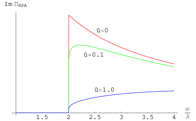
Figure 3: The imaginary part of the spin-response function $\Pi_{\mathrm{RPA}}$ in SSI in $d=2$, calculated using the random-phase approximation. The red line, with zero coupling, gives the one-loop diagram $\Pi_{0}$, while the other two lines give the results for nonzero coupling $\hat{u}$. This coupling constant is a linear combination of $u$ and $v$, the two couplings appearing in the action $\mathcal{S}_{\mathrm{SSI}}$, Eq. (29).

IV.2 SSI near SSC

As the spin-dependent interaction increases and the SSC phase is approached, a bound state composed of a singlet pair of bosons becomes energetically favorable. At the transition to SSC, the singlet pairs condense into a superfluid with no spin ordering.

To describe the approach to this transition, we start with the action $\mathcal{S}_{\mathrm{SSI}}$ and introduce the field $\Psi\sim\psi_{\mu}\psi_{\mu}$, by a Hubbard-Stratonovich decoupling of the quartic interaction $v$. The field $\Psi$ describes the singlet pairs and will condense across the transition. It is described by the action

$$\mathcal{S}_{\Psi}=\int\mathrm{d}^{d}\mathbf{x}\,\mathrm{d}t\>\left(|\partial\Psi|^{2}+r_{\Psi}|\Psi|^{2}+\frac{u_{\Psi}}{4}|\Psi|^{4}+\,\cdots\right)\;\mathrm{.}$$ (41)

The full action has the form

$$\mathcal{S}_{\mathrm{SSI}}^{\prime}=\mathcal{S}_{\psi}+\mathcal{S}_{\Psi}+\frac{g_{\psi}}{2}\int\mathrm{d}^{d}\mathbf{x}\,\mathrm{d}t\>\left(\bar{\Psi}\psi_{\mu}\psi_{\mu}+\Psi\bar{\psi}_{\mu}\bar{\psi}_{\mu}\right)\;\mathrm{.}$$ (42)

(The introduction of the field $\Psi$ renormalizes the coupling constants within $\mathcal{S}_{\psi}$. Here and throughout, we will simplify the notation by retaining the same symbols for these renormalized quantities.)

IV.2.1 Self energy

The diagrams shown in Section IV.1.1, coming from $\mathcal{S}_{\psi}$, will still contribute to the self energy near to SSC. As seen above, however, these diagrams are important only for $\omega>3\lambda$, whereas new diagrams coming from coupling to the pair field $\Psi$ will contribute at lower frequencies.

Using a double line for the propagator of the $\Psi$ field, the first diagram is

$$\Sigma_{1}^{\psi}=\;\parbox{85.35826pt}{ \begin{picture}(30.0,20.0)\put(0.0,0.0){\includegraphics{fmfspindyn.5.ps}} \end{picture}}\;\mathrm{,}$$ (43)

in which a particle decays into a hole plus a pair. The vertices correspond to factors of $g_{\psi}$. The threshold for this process is clearly $\lambda+\lambda_{\Psi}$, where $\lambda$ is the gap to the particle and hole excitation as before, and $\lambda_{\Psi}=\sqrt{r_{\Psi}}$ is the gap to the pair excitation. This excitation therefore becomes important at low energies when $\lambda_{\Psi}<2\lambda$, which is simply the condition that a bound state exists below the two-particle continuum.

The diagram can be evaluated in $d=2$ to give

$$\Sigma_{1}^{\psi}=\frac{g_{\psi}^{2}}{8\pi\omega}\log\frac{\lambda+\lambda_{\Psi}+\omega}{\lambda+\lambda_{\Psi}-\omega}\;\mathrm{,}$$ (44)

and the corresponding spectral weight is shown in Figure 4; the structure of this threshold singularity is similar to Eq. (38), and as was the case there, in general $d$ we have a singularity $\sim(\omega-\lambda-\lambda_{\Psi})^{(d-2)/2}$. A continuum of excitations appears for $\omega>\lambda+\lambda_{\Psi}$, as expected. As the transition to SSC is approached, $\lambda_{\Psi}$ becomes smaller and the edge of the continuum approaches the peak at $\omega=\lambda$. The perturbation expansion used here breaks down as $\lambda_{\Psi}\rightarrow 0$ and a more sophisticated RG calculation, described in Section VII, is required.

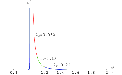
Figure 4: The spectral weight $\rho^{\psi}$ in SSI near the transition to SSC, calculated up to order $g_{\psi}^{2}$, plotted for three different values of $\lambda_{\Psi}$, the gap to pair excitations. The coupling strength is $g_{\psi}=0.1$. The peak at $\omega=\lambda$ (which is present for all values of $\lambda_{\Psi}$ and has artificially been given a small but nonzero width) describes the stable particle and hole excitation of the field $\psi_{\mu}$. For $\omega>\lambda+\lambda_{\Psi}$, there is continuum of excitations, corresponding physically to the conversion of a particle to a pair plus a hole.

IV.2.2 Spin response

Since $\Psi$ is a spin singlet, it gives no direct contribution to the spin response, which is therefore given by Eq. (34), as before. The presence of the bound state, however, allows for new diagrams that contribute to the response function $\Pi_{\mu\nu,\rho\sigma}$.

One such diagram is

$$\Pi^{(1a)}=\;\parbox{85.35826pt}{ \begin{picture}(30.0,20.0)\put(0.0,0.0){\includegraphics{fmfspindyn.6.ps}} \end{picture} }\;\mathrm{,}$$ (45)

which is the first term in the series

$$\parbox{56.9055pt}{ \begin{picture}(20.0,15.0)\put(0.0,0.0){\includegraphics{fmfspindyn.7.ps}} \end{picture} }+\parbox{71.13188pt}{ \begin{picture}(25.0,15.0)\put(0.0,0.0){\includegraphics{fmfspindyn.8.ps}} \end{picture} }+\parbox{85.35826pt}{ \begin{picture}(30.0,15.0)\put(0.0,0.0){\includegraphics{fmfspindyn.9.ps}} \end{picture} }+\parbox{113.81102pt}{ \begin{picture}(40.0,15.0)\put(0.0,0.0){\includegraphics{fmfspindyn.10.ps}} \end{picture} }+\cdots$$ (46)

For $x=\omega-2\lambda$ positive but very small, the pair propagator can be replaced by a constant. Summing over these diagrams will therefore lead to a similar $1/\log x$ singularity to that described above in Section IV.1.2. This replacement is only valid for $x<\lambda_{\Psi}$. For $\omega>2\lambda+\lambda_{\Psi}$, a 3-particle threshold singularity is found, similar to that discussed below Eq. (33). Qualitatively different behavior will result as the transition to SSC is approached and $\lambda_{\Psi}\rightarrow 0$. This will be addressed below in Section VII.

IV.3 Spin-singlet condensate

In the SSC phase, singlet pairs of bosons form a condensate, giving a superfluid with no spin ordering. This will only occur when the spin-dependent interaction is strong enough to overcome the extra kinetic-energy cost of having bound singlet pairs. This requires sufficiently large $J/U$, as shown in Figure 1.

The perturbation expansion used in Section IV.2 is not applicable here, and we must instead expand about the new ground state, with a condensed $\Psi$ field. (A similar approach can be used to describe the condensed phase of the spinless Bose gas Popov .)

We first write $\Psi$ in terms of amplitude and phase as

$$\Psi=\Psi_{0}\mathrm{e}^{\mathrm{i}\theta^{\prime}}\;\mathrm{,}$$ (47)

where $\Psi_{0}$ and $\theta^{\prime}$ are both real. For simplicity, we treat the amplitude of the $\Psi$ field as a constant, ignoring the gapped amplitude modes. (This is appropriate sufficiently far from the transition to SSI, where the gap is large.) With this parametrization, $\mathcal{S}_{\Psi}$, given by Eq. (41), can be rewritten as the action of a free, gapless field:

$$\mathcal{S}_{\Psi}=\int\mathrm{d}^{d}\mathbf{x}\,\mathrm{d}t\>\frac{1}{2}(\partial\theta)^{2}\;\mathrm{,}$$ (48)

with the definition $\theta=\sqrt{2}\Psi_{0}\theta^{\prime}$. Physically, $\theta$ is interpreted as the Goldstone mode corresponding to the broken phase symmetry in SSC.

In dealing with $\psi_{\mu}$, it is convenient to take out a factor of the condensate phase by writing $\psi_{\mu}=\varphi_{\mu}\mathrm{e}^{\mathrm{i}\theta^{\prime}/2}$. Then, since the condensate has broken phase-rotation invariance, we rewrite the field $\varphi_{\mu}$ in terms of real and imaginary parts,

$$\varphi_{\mu}=\frac{1}{\sqrt{2}}(\varphi_{\mu}^{R}+\mathrm{i}\varphi_{\mu}^{I})\;\mathrm{.}$$ (49)

In terms of the new fields $\theta$, $\varphi_{\mu}^{R}$ and $\varphi_{\mu}^{I}$, the action becomes

$$\mathcal{S}_{\mathrm{SSC}}=\int\mathrm{d}^{d}\mathbf{x}\,\mathrm{d}t\>\bigg{\{}\frac{1}{2}(\partial\theta)^{2}+\frac{1}{2}\varphi_{\mu}^{R}(-\partial^{2}+r+g^{\psi}\Psi_{0}/2)\varphi_{\mu}^{R}+\frac{1}{2}\varphi_{\mu}^{I}(-\partial^{2}+r-g^{\psi}\Psi_{0}/2)\varphi_{\mu}^{I}\\ +\frac{u}{16}\,(\varphi_{\mu}^{R}\varphi_{\mu}^{R}+\varphi_{\mu}^{I}\varphi_{\mu}^{I})(\varphi_{\nu}^{R}\varphi_{\nu}^{R}+\varphi_{\nu}^{I}\varphi_{\nu}^{I})+\frac{v}{16}\,\left[(\varphi_{\mu}^{R}\varphi_{\mu}^{R}-\varphi_{\mu}^{I}\varphi_{\mu}^{I})(\varphi_{\nu}^{R}\varphi_{\nu}^{R}-\varphi_{\nu}^{I}\varphi_{\nu}^{I})+4\varphi_{\mu}^{R}\varphi_{\mu}^{I}\varphi_{\nu}^{R}\varphi_{\nu}^{I}\right]\\ +\frac{i}{\sqrt{8}\Psi_{0}}(\varphi_{\mu}^{I}\partial\varphi_{\mu}^{R}-\varphi_{\mu}^{R}\partial\varphi_{\mu}^{I})\cdot\partial\theta+\frac{1}{16\Psi_{0}^{2}}(\varphi_{\mu}^{R}\varphi_{\mu}^{R}+\varphi_{\mu}^{I}\varphi_{\mu}^{I})(\partial\theta)^{2}\bigg{\}}\;\mathrm{.}$$ (50)

Note that the two fields $\varphi_{\mu}^{R}$ and $\varphi_{\mu}^{I}$ remain gapped, but that their gaps are not the same. The lowest-energy ‘charged’ mode is $\varphi_{\mu}^{I}$, with gap $\lambda_{I}=\sqrt{r-g^{\psi}\Psi_{0}/2}$.

IV.3.1 Self energy

As an example, we consider the lowest-order diagram that contributes to the decay rate for $\varphi_{\mu}^{I}$, at energies well below that required to produce an excitation of the field $\varphi_{\mu}^{R}$. This is given by

$$\Sigma^{\varphi}=\;\parbox{85.35826pt}{ \begin{picture}(30.0,20.0)\put(0.0,0.0){\includegraphics{fmfspindyn.11.ps}} \end{picture}}\;\mathrm{,}$$ (51)

where the solid lines represent $\varphi_{\mu}^{I}$ and the dashed lines $\theta$. Each vertex represents a factor $\sim(p_{1}\cdot p_{2})\Psi_{0}^{-2}$, where $p_{1}$ and $p_{2}$ are the momenta of the two $\theta$ propagators, coming from the final term in $\mathcal{S}_{\mathrm{SSC}}$. (All the other interaction terms involve $\varphi_{\mu}^{R}$ and contribute to the decay rate only at higher energies. As in Section IV.1.1, there is also a lower-order tadpole diagram that does not contribute to the decay rate.)

The diagram can be calculated numerically and the corresponding spectral weight is shown in Figure 5. As in SSI, there is a sharp peak (at $\omega=\lambda_{I}$) corresponding to the stable gapped ‘charged’ mode, followed at higher energy by a continuum of excitations. In this case, however, the Goldstone mode $\theta$ causes the continuum to begin precisely at $\omega=\lambda_{I}$, albeit suppressed by a factor of $(\omega-\lambda_{I})^{3}$.

Figure 5: The spectral weight $\rho^{\varphi}$ for the field $\varphi_{\mu}^{I}$ in SSC, near the gap $\lambda_{I}$, calculated numerically using the diagram in Eq. (51). As in Figures 2 and 4, there is a delta-function peak at $\omega=\lambda_{I}$ (which has artificially been given a nonzero width), corresponding to the stable particle excitation. In this case, unlike in SSI, the continuum in the spectral weight occurs immediately above the peak. This is due to the (gapless) Goldstone mode $\theta$ resulting from the broken phase symmetry in SSC. The derivatives in the coupling between the Goldstone mode and the $\varphi_{\mu}^{I}$ field in $\mathcal{S}_{\mathrm{SSC}}$ strongly suppress the spectral weight as $\omega\rightarrow\lambda_{I}$ from above; in fact, $\rho^{\varphi}\sim(\omega-\lambda_{I})^{3}$.

This should be contrasted with the behavior at the transition itself, described below in Section VII. At the transition, the gapless modes are critical, rather than Goldstone modes, and their coupling is not suppressed by powers of the momentum. As a result, the spectral weight, calculated perturbatively, does not tend to zero as $\omega\rightarrow\lambda$ (see Section VII.2) and a RG analysis shows that the sharp quasiparticle peak at $\omega=\lambda$ is in fact replaced by a weaker power-law singularity, reflecting the absence of quasiparticles at the critical point.

IV.3.2 Spin response

The first contribution to the spin response resulting from the coupling of $\varphi_{\mu}^{I}$ to $\theta$ has three loops:

$$\Pi^{(1a)}=\;\parbox{85.35826pt}{ \begin{picture}(30.0,20.0)\put(0.0,0.0){\includegraphics{fmfspindyn.12.ps}} \end{picture} }\;\mathrm{.}$$ (52)

As for the self energy, the powers of momentum appearing in the interaction vertex strongly suppress the contribution at low energy, and this diagram will not modify the threshold singularity in the spin response.

IV.4 Polar condensate

In the polar condensate phase, $\psi_{\mu}$ condenses, breaking both the spin- ($S$) and phase-rotation ($\Phi$) symmetries. A different set of fields is therefore required to describe this phase, in which there are gapless excitations carrying both particle number and spin. A similar approach can be used to that described above for SSC, but since the calculations are rather involved, we will only give a brief outline.

In terms of the general continuum theory of Section III.1 given in Eq. (15), this phase corresponds to a condensate of $\psi_{\mu}$. This field is a complex vector and can take an arbitrary direction in space, which for simplicity we take as real and along the $z$-axis: $\left\langle\psi_{\mu}\right\rangle=\varphi_{0}\delta_{\mu z}$. A convenient representation for the field is then to write

$$\psi_{\mu}=\varphi_{0}\,\mathrm{e}^{\mathrm{i}\chi}\,\mathrm{e}^{\mathrm{i}\alpha_{i}\sigma_{i}}\,\mathrm{e}^{\mathrm{i}\beta_{j}\tau_{j}}\,\delta_{\mu z}\;\mathrm{.}$$ (53)

As in Section IV.3, the amplitude modes of the condensed field, which are inessential to the physics, have been neglected. Summation over $i,j\in\{x,y\}$ is implied; $\chi$, $\alpha_{i}$ and $\beta_{j}$ are real fields; and $\sigma_{i}$ and $\tau_{j}$ are matrices acting in spin space: $\sigma_{x}=\left(\begin{smallmatrix}0&0&-\mathrm{i}\\ 0&0&0\\ \mathrm{i}&0&0\end{smallmatrix}\right)$, $\sigma_{y}=\left(\begin{smallmatrix}0&0&0\\ 0&0&-\mathrm{i}\\ 0&\mathrm{i}&0\end{smallmatrix}\right)$, $\tau_{x}=\left(\begin{smallmatrix}0&0&1\\ 0&0&0\\ 1&0&0\end{smallmatrix}\right)$ and $\tau_{y}=\left(\begin{smallmatrix}0&0&0\\ 0&0&1\\ 0&1&0\end{smallmatrix}\right)$.

The physical interpretation of this parametrization is as follows: The factor $\mathrm{e}^{\mathrm{i}\chi}$ incorporates the overall phase degree of freedom, similarly to $\mathrm{e}^{\mathrm{i}\theta^{\prime}}$ in Eq. (47). The matrices $\sigma_{i}$ are the generators of real rotations in spin space and serve to rotate the axis along which the vector $\psi_{\mu}$ is aligned. These two kinds of transformation correspond to symmetries of the action, and the energy is unchanged by uniform shifts in $\chi$, $\alpha_{x}$ and $\alpha_{y}$. There are therefore three Goldstone modes in this phase, two of which carry spin.

The remaining matrices, $\tau_{x}$ and $\tau_{y}$, generate complex transformations of the condensate wavefunction, and describe the angular momentum degree of freedom. The corresponding modes, described by $\beta_{x}$ and $\beta_{y}$, would be Goldstone modes in a system with full $\mathrm{SU}(3)$ symmetry and have gaps proportional to $v$, the coefficient appearing in Eq. (16).

In this representation, the action can be rewritten

$$\mathcal{S}_{\mathrm{PC}}=\int\mathrm{d}^{d}\mathbf{x}\,\mathrm{d}t\>\left\{\frac{1}{2}(\partial\chi)^{2}+\frac{1}{2}(\partial\alpha_{i})^{2}+\frac{1}{2}\left[(\partial\beta_{i})^{2}-4v\beta_{i}^{2}\right]-\frac{2}{\varphi_{0}}\beta_{i}(\partial\alpha_{i})\cdot(\partial\chi)+\cdots\right\}\;\mathrm{,}$$ (54)

where summation over $i$ is again implied. [As in Eq. (48), the fields have been rescaled by constant factors to give the coefficients of the kinetic terms their conventional values.]

The angular momentum, given by Eq. (20), can be rewritten in terms of the fields defined in Eq. (53), giving for the transverse components

$$L_{x}\sim-\beta_{y}\qquad\mathrm{and}\qquad L_{y}\sim\beta_{x}\;\mathrm{,}$$ (55)

and for the longitudinal component

$$L_{z}\sim\alpha_{x}\beta_{y}-\alpha_{y}\beta_{x}\;\mathrm{.}$$ (56)

The longitudinal and transverse components are given by different expressions because of the broken spin-rotation symmetry. These different expressions will lead to qualitatively different forms for the transverse and longitudinal spin responses.

V Quantum phase transitions

We now describe the behavior of the system across transitions out of the spin-singlet insulator (SSI) into the various phases described above. First we briefly address each of the transitions in turn, before describing them in more detail, in Sections VI, VII and VIII.

First, consider the transition from SSI into the nematic insulator (NI). Both phases have $\left\langle\psi_{\mu}\right\rangle=0$, and off-diagonal elements of $\left\langle\bar{\psi}_{\mu}\psi_{\nu}\right\rangle$ become nonzero across the transition. As suggested by the mean-field analysis Section II.3, this is expected to be a first-order transition. This is confirmed by the presence of terms cubic in $\bar{\psi}_{\mu}\psi_{\nu}$ in the action $\mathcal{S}_{\psi}$, Eq. (15), which are not forbidden by any symmetry (and are hidden in the ellipsis). We will not consider this transition further here.

V.1 SSI to PC

At the transition to PC, the field $\psi_{\mu}$ becomes critical; the appropriate field theory is therefore given by Eq. (29). Since the critical field $\psi_{\mu}$ carries spin, this transition is an example of class A identified above, in Section I. The field $\psi_{\mu}$ is gapless and the spin response will be governed by the correlators of $\bar{\psi}_{\mu}\psi_{\nu}$, as in SSI. A RG analysis of this transition will be presented below in Section VI.

V.2 SSI to SSC

The critical field at the transition to SSC is the singlet pair $\Psi$, introduced in Section IV.2. Once $\Psi$ has been isolated, $\psi_{\mu}$, which has no gapless excitations, can be safely integrated out. This leaves the field theory of a single complex scalar, with the same form as the action $\mathcal{S}_{\Psi}$ given in Eq. (41):

$$\mathcal{S}_{\Psi}=\int\mathrm{d}^{d}\mathbf{x}\,\mathrm{d}t\>\left(|\partial\Psi|^{2}+r_{\Psi}|\Psi|^{2}+\frac{u_{\Psi}}{4}|\Psi|^{4}+\,\cdots\right)\;\mathrm{.}$$ (57)

This transition is therefore of the XY universality class, with upper critical dimension $D=d+1=4$. (The field $\Psi$ has engineering dimension $[\Psi]=(d-1)/2$, so the coupling $u_{\Psi}$ has dimension $[u_{\Psi}]=3-d$.)

Since the critical field $\Psi$ is spinless, this phase transition falls within class B identified in Section I. While the action $\mathcal{S}_{\Psi}$ is sufficient to describe the critical properties of the ground state across the transition, we are primarily interested in excitations that carry spin, and the critical theory given by $\mathcal{S}_{\Psi}$ does not describe these. Instead, we must keep the singly-charged excitations given by $\psi_{\mu}$, and use the full action $\mathcal{S}_{\mathrm{SSI}}^{\prime}$, in Eq. (42).

As in Section IV.2, the spin response is determined by the lowest-energy spin-carrying (but overall charge-neutral) excitations. These will normally be described by particle–hole pairs of $\psi_{\mu}$, but we also address the case in which there is a lower-energy bound state, which then governs the long-time response. Such a bound state is more likely to form in a region of the SSI-to-SSC phase boundary which is well away from the PC phase in Fig. 1.

V.2.1 Without bound state

When there is no bound state, the spin response is determined by the correlators of the compound operator $\bar{\psi}_{\mu}\psi_{\nu}$, as in Eq. (34). The corresponding action is therefore given by $\mathcal{S}_{\mathrm{SSI}}^{\prime}$, in Eq. (42).

Since $\psi_{\mu}$ has only gapped excitations, while the field $\Psi$ is now gapless, this can be simplified somewhat. The important excitations are those just above the gap $\lambda=\sqrt{r}$, for which the dispersion can be replaced by a nonrelativistic form. We define particle and hole operators so that $\psi_{\mu}\sim p_{\mu}+\bar{h}_{\mu}$, giving an action $\mathcal{S}_{\Psi}+\mathcal{S}_{\Psi,\psi}^{\prime}$, where

$$\mathcal{S}^{\prime}_{\Psi,\psi}=\int\mathrm{d}^{d}\mathbf{x}\,\mathrm{d}t\>\bigg{[}\bar{p}_{\mu}\left(\mathrm{i}\partial_{t}-\frac{\nabla^{2}}{2m_{\psi}}+\lambda\right)p_{\mu}+\bar{h}_{\mu}\left(\mathrm{i}\partial_{t}-\frac{\nabla^{2}}{2m_{\psi}}+\lambda\right)h_{\mu}\\ +g_{\psi}\left(\bar{\Psi}p_{\mu}\bar{h}_{\mu}+\Psi\bar{p}_{\mu}h_{\mu}\right)\bigg{]}\;\mathrm{.}$$ (58)

Using power counting (and taking $[t]=[\mathbf{x}]=-1$, since the critical theory $\mathcal{S}_{\Psi}$ is relativistic), the engineering dimension of the kinetic-energy term is $[1/m_{\psi}]=-1$. The dispersion is therefore irrelevant and, at least prima facie, the particles and holes can be treated as static impurities. We therefore take for the action

$$\mathcal{S}_{\Psi,\psi}=\int\mathrm{d}^{d}\mathbf{x}\,\mathrm{d}t\>\left[\bar{p}_{\mu}\left(\mathrm{i}\partial_{t}+\lambda\right)p_{\mu}+\bar{h}_{\mu}\left(\mathrm{i}\partial_{t}+\lambda\right)h_{\mu}+g_{\psi}\left(\bar{\Psi}p_{\mu}\bar{h}_{\mu}+\Psi\bar{p}_{\mu}h_{\mu}\right)\right]\;\mathrm{.}$$ (59)

The scaling dimension of the coupling $g_{\psi}$ is $[g_{\psi}]=(3-d)/2$, so that it is relevant for $d<3$. It is therefore relevant in two (spatial) dimensions and marginal in three, and we will consider both of these cases below. Any other interactions, including terms quartic in $p_{\mu}$ and $h_{\mu}$, are irrelevant.

In Section VII, we will treat the case $d=2$ using a renormalization-group (RG) analysis, and then, in Section VII.2, return to the case $d=3$, where straightforward perturbation theory is sufficient.

V.2.2 With bound state

If a bound state of $p_{\mu}$ and $h_{\nu}$ exists below the continuum, it will determine the lowest-energy spin response. At higher energies, the continuum of particle and hole excitations remains and will have the same effects as described above in Section V.2.1.

The particle and hole excitations $p_{\mu}$ and $h_{\nu}$ carry spin $1$, so the simplest spin-carrying bound states are a quintet with spin $2$. (Bound states with antisymmetric relative spatial wavefunctions and net spin $S=1$ are also possible.) To describe these bound states, we introduce the field $d_{\mu\nu}$, a (symmetric, traceless) second-rank tensor:

$$d_{\mu\nu}\sim\bar{\psi}_{\mu}\psi_{\nu}-\frac{1}{3}\delta_{\mu\nu}\bar{\psi}_{\rho}\psi_{\rho}\;\mathrm{.}$$ (60)

By symmetry, angular momentum $\mathbf{L}$ couples to $d_{\mu\nu}$ by $L_{\rho}\sim\mathrm{i}\epsilon_{\mu\nu\rho}\bar{d}_{\mu\lambda}d_{\lambda\nu}$, and it is necessary to create a pair of $d$ excitations to propagate the spin excitation. This will require more energy than an unbound particle-hole pair and so the response function $\Pi_{\mathbf{L}}$ will still be given by the compound operator $\bar{\psi}_{\mu}\psi_{\nu}$, as in Section V.2.1.

On the other hand, it is clear from its definition, in Eq. (22), that $Q_{\mu\nu}$ couples directly to $d_{\mu\nu}$. The response function $\Pi_{Q}$ is therefore given by the two-point correlator of $d_{\mu\nu}$:

$$\Pi_{Q}\sim\left\langle\mathcal{T}_{t}\>\bar{d}_{\mu\nu}(\mathbf{x},t)d_{\mu\nu}(\mathbf{0},0)\right\rangle\;\mathrm{.}$$ (61)

To construct the corresponding action, we notice first that there is no term such as $\bar{\Psi}\Psi d_{\mu\mu}$, because $d_{\mu\nu}$ is traceless, so that the next order in the expansion must be taken. The action for $d_{\mu\nu}$ is then given by

$$\mathcal{S}_{\Psi,d}=\int\mathrm{d}^{d}\mathbf{x}\,\mathrm{d}t\>\left[\bar{d}_{\mu\nu}\left(\mathrm{i}\partial_{t}-\frac{\nabla^{2}}{2m_{d}}+r_{d}\right)d_{\mu\nu}+g_{d}\bar{d}_{\mu\nu}d_{\mu\nu}\bar{\Psi}\Psi+\,\cdots\right]\;\mathrm{.}$$ (62)

The same power-counting argument as above shows that $[1/m_{d}]=-1$ and the dispersion is irrelevant. The scaling dimension of the interaction $g_{d}$ is $[g_{d}]=2-d$, so that it becomes marginal at $d=2$ and is irrelevant for $d=3$. This case therefore falls within class B2; we describe the properties of the critical region below, in Section VIII.

VI Critical properties: SSI/PC (Class A)

The transition from SSI to PC is described by the action given in Eq. (15), with two different quartic terms allowed by the $\mathrm{U}(1)\otimes\mathrm{O}(3)$ symmetry:

$$\mathcal{S}_{\psi}=-\bar{\psi}_{\mu}\partial^{2}\psi_{\mu}+r\bar{\psi}_{\mu}\psi_{\mu}+\frac{u}{4}\bar{\psi}_{\mu}\psi_{\mu}\bar{\psi}_{\nu}\psi_{\nu}+\frac{v}{4}\bar{\psi}_{\mu}\bar{\psi}_{\mu}\psi_{\nu}\psi_{\nu}\;\mathrm{.}$$ (63)

To study the critical behavior of the model, a straightforward RG calculation can be performed, leading to the following beta functions to one loop:

$$\beta_{u} =-\epsilon\tilde{u}+\frac{7}{2}\tilde{u}^{2}+2\tilde{u}\tilde{v}+2\tilde{v}^{2}$$ (64)

$$\beta_{v} =-\epsilon\tilde{v}+3\tilde{u}\tilde{v}+\frac{3}{2}\tilde{v}^{2}$$ (65)

(where $\tilde{u}$ and $\tilde{v}$ are related to $u$ and $v$ by constant factors). These flow equations have no stable fixed point for finite $u$ and $v$. However, far more complete six-loop analyses in Ref. PratoPelissetto, have shown that a stable fixed point does indeed exist with $v<0$. At this fixed point, the full Green function for the field $\psi_{\mu}$ behaves like

$$G^{\psi}(p)\sim p^{-2+\eta_{\psi}}\;\mathrm{,}$$ (66)

where $\eta_{\psi}=0$ to one-loop order, while the six-loop estimate is PratoPelissetto $\eta_{\psi}\approx 0.08$. The polarization $\Pi_{\mu\nu,\rho\sigma}$ is determined by the response functions $\Pi_{\mathbf{L}}$ and $\Pi_{Q}$ defined in Section IV, and these have singularities of the form

$$\Pi_{\mathbf{L}}(q)\sim q^{-2+\eta_{\mathbf{L}}}\;\mathrm{,}~{}~{}\Pi_{Q}(q)\sim q^{-2+\eta_{Q}}\;\mathrm{,}$$ (67)

where the $\eta_{\mathbf{L},Q}$ are exponents related to scaling dimensions of operators bilinear in $\psi_{\mu}$ at the fixed point of Ref. PratoPelissetto, . In particular, we have $\eta_{\mathbf{L}}=\eta_{H}$ where the latter exponent is defined in Ref. PratoPelissetto, , and for which their estimate is $\eta_{H}\approx 2.70$. For $\Pi_{Q}$ we have $\eta_{Q}=d+3-2y_{3}$, where $y_{3}\approx 2.0$ is the exponent listed in Table III of Ref. CalabreseVicari, for the collinear case with $N=3$.

VII Critical properties: SSI–SSC (Class B1)

The critical theory for the phase transition between SSI and SSC is given by

$$\mathcal{S}_{\Psi}=\int\mathrm{d}^{d}\mathbf{x}\,\mathrm{d}\tau\>\left(|\partial\Psi|^{2}+r_{\Psi}|\Psi|^{2}+\frac{u_{\Psi}}{4}|\Psi|^{4}\right)\;\mathrm{,}$$ (68)

where we have rewritten the action in imaginary time. Since the field $\Psi$ carries no spin, the lowest energy excitations are described by

$$\mathcal{S}_{\Psi,\psi}=\int\mathrm{d}^{d}\mathbf{x}\,\mathrm{d}\tau\>\left[\bar{p}_{\mu}\left(\partial_{\tau}+\lambda\right)p_{\mu}+\bar{h}_{\mu}\left(\partial_{\tau}+\lambda\right)h_{\mu}+g_{\psi}\left(\bar{\Psi}p_{\mu}\bar{h}_{\mu}+\Psi\bar{p}_{\mu}h_{\mu}\right)\right]\;\mathrm{.}$$ (69)

For $d<3$, the correlation functions of the particle and hole excitations can be found using a RG calculation. Since the present approach is slightly different from the standard RG, we perform the calculation using a cutoff in momentum space, which makes the logic involved more transparent, in Appendix A. Here we use dimensional regularization, which is the simplest approach from a calculational point of view.

We define the (imaginary-time) free propagator for the $\Psi$ field as

$$G^{\Psi}_{0}(\mathbf{k},\mathrm{i}\omega)=\frac{1}{k^{2}+\omega^{2}+r_{\Psi}}\;\mathrm{.}$$ (70)

At the critical point, the renormalized mass of $\Psi$ vanishes; in dimensional regularization, this occurs for $r_{\Psi}=0$. For the $p_{\mu}$ and $h_{\mu}$ fields, the propagator is

$$G^{\psi}_{0}(\mathrm{i}\omega)=\frac{1}{-\mathrm{i}\omega+\lambda}\;\mathrm{,}$$ (71)

independent of the momentum.

The renormalization of the terms in the action $\mathcal{S}_{\Psi}$ describing $\Psi$ is identical to the standard analysis:Zinn-Justin the presence of the gapped $\psi_{\mu}$ excitations cannot affect the critical behavior of the gapless $\Psi$ field. The corresponding RG has a fixed point with $u_{\Psi}$ of order $\epsilon=3-d$, at which the scaling dimension of $\Psi$ is $[\Psi]=1-\epsilon/2+\epsilon^{2}/100+\mathcal{O}\left(\epsilon^{3}\right)$.

To lowest order in the coupling $g_{\psi}$ (or, as will subsequently be shown to be equivalent, in an expansion in $\epsilon$), the only self-energy diagram for the particle field $p_{\mu}$ is as shown in Eq. (43):

$$\Sigma^{\psi}_{1}(\mathrm{i}\omega) =\qquad\parbox{85.35826pt}{ \begin{picture}(30.0,20.0)\put(0.0,0.0){\includegraphics{fmfspindyn.13.ps}} \put(15.00029,17.94228){\makebox(0.0,0.0)[b]{$\mathbf{k},\mathrm{i}\omega^{\prime}$}} \end{picture}}$$ (72)

$$=g_{\psi}^{2}\int_{\mathbf{k}}\int_{-\infty}^{\infty}\frac{\mathrm{d}\omega^{\prime}}{2\pi}\,G^{\Psi}_{0}(\mathbf{k},\mathrm{i}\omega^{\prime})G^{\psi}_{0}\biglb(\mathrm{i}(\omega-\omega^{\prime})\bigrb)\;\mathrm{,}$$ (73)

where

$$\int_{\mathbf{k}}\equiv\int\frac{\mathrm{d}^{d}\mathbf{k}}{(2\pi)^{d}}\equiv\Omega_{d}\int_{0}^{\infty}\mathrm{d}k\,k^{d-1}$$ (74)

(for an isotropic integrand).

There happen to be no diagrams giving a renormalization of the coupling $g_{\psi}$ at this order, but such diagrams appear in higher orders, as in Eq. (78).

Charge-neutral compound operators such as $L_{\rho}$ and $Q_{\mu\nu}$, defined in Section III.3, can be written in the form $T_{\mu\nu}p_{\mu}h_{\nu}$, where $T_{\mu\nu}$ is a matrix of $c$-numbers. The critical exponents for these operators can then be found by considering the renormalization of the corresponding insertion, given by

$$H_{1}(2\mathrm{i}\omega) =\qquad\parbox{71.13188pt}{ \begin{picture}(25.0,25.0)\put(0.0,0.0){\includegraphics{fmfspindyn.14.ps}} \put(20.99109,3.80617){\makebox(0.0,0.0)[lb]{$\mu$}}\put(9.18875,5.8954){\makebox(0.0,0.0)[rt]{$\mu$}}\put(18.47226,12.49998){\makebox(0.0,0.0)[l]{$\mathbf{k},\mathrm{i}\omega^{\prime}$}}\put(9.18878,19.10498){\makebox(0.0,0.0)[rb]{$\nu$}}\put(20.99109,21.19383){\makebox(0.0,0.0)[lt]{$\nu$}} \end{picture}}$$ (75)

$$=g_{\psi}^{2}\int_{\mathbf{k}}\int_{-\infty}^{\infty}\frac{\mathrm{d}\omega^{\prime}}{2\pi}\,G^{\Psi}_{0}(\mathbf{k},\mathrm{i}\omega^{\prime})G^{\psi}_{0}\biglb(\mathrm{i}(\omega-\omega^{\prime})\bigrb)G^{\psi}_{0}\biglb(\mathrm{i}(\omega+\omega^{\prime})\bigrb)\;\mathrm{,}$$ (76)

where all spin indices have been omitted in the latter expression. In accounting for these indices, it is important to note that the exchange of the pair interchanges the particle and hole lines and hence $\mu$ and $\nu$. This causes the results to be dependent on the symmetry of the matrix $T_{\mu\nu}$, leading to different scaling exponents for excitations with even ($T_{\mu\nu}$ symmetric, eg, $Q_{\mu\nu}$) and odd spin ($T_{\mu\nu}$ antisymmetric, eg, $L_{\rho}$).

To order $\epsilon^{2}$, the diagrams that must be evaluated are, for the self energy:

$$\Sigma^{\psi}_{2}(\mathrm{i}\omega)=\quad\parbox{99.58464pt}{ \begin{picture}(35.0,20.0)\put(0.0,0.0){\includegraphics{fmfspindyn.15.ps}} \end{picture}}$$ (77)

and for the renormalization of $g_{\psi}$:

$$\Gamma^{\psi}_{2}(\mathrm{i}\omega)=\quad\parbox{99.58464pt}{ \begin{picture}(35.0,25.0)\put(0.0,0.0){\includegraphics{fmfspindyn.16.ps}} \end{picture}}+\quad\parbox{99.58464pt}{ \begin{picture}(35.0,25.0)\put(0.0,0.0){\includegraphics{fmfspindyn.17.ps}} \end{picture}}$$ (78)

(Note that the second diagram involves the four-point coupling of the $\Psi$ field, indicated in the diagram by the empty circle.) The renormalization of the insertion is given by the following diagrams:

$$H_{2}(2\mathrm{i}\omega)=\quad\parbox{99.58464pt}{ \begin{picture}(35.0,25.0)\put(0.0,0.0){\includegraphics{fmfspindyn.18.ps}} \end{picture}}+\quad\parbox{99.58464pt}{ \begin{picture}(35.0,25.0)\put(0.0,0.0){\includegraphics{fmfspindyn.19.ps}} \end{picture}}+\quad\parbox{99.58464pt}{ \begin{picture}(35.0,25.0)\put(0.0,0.0){\includegraphics{fmfspindyn.20.ps}} \end{picture}}$$ (79)

We will display the steps in the calculation of the results to order $\epsilon$ and simply state the higher-order results afterwards. For the self energy, performing the integral over $\omega^{\prime}$ using contour integration gives

$$\Sigma^{\psi}_{1}(\mathrm{i}\omega)=g_{\psi}^{2}\int_{\mathbf{k}}\frac{1}{2k}\cdot\frac{1}{-\mathrm{i}\omega+\lambda+k}\;\mathrm{,}$$ (80)

which leads to, defining $z=-\mathrm{i}\omega+\lambda$,

$$\Sigma^{\psi}_{1}(\mathrm{i}\omega)=-\frac{g_{\psi}^{2}z^{1-\epsilon}}{4\pi^{2}\epsilon}\;\mathrm{,}$$ (81)

plus terms that are finite as $\epsilon\rightarrow 0$.

To this order, the full propagator of the particle is then given by

$$(G^{\psi})^{-1} =z-\Sigma^{\psi}_{1}$$ (82)

$$=z\left(1+\frac{g_{\psi}^{2}z^{-\epsilon}}{4\pi^{2}\epsilon}\right)\;\mathrm{,}$$ (83)

so that renormalizing the propagator (using minimal subtraction) at frequency $z=\mu$ gives for the wavefunction renormalization

$$Z_{\psi}=1-\frac{g_{\psi}^{2}\mu^{-\epsilon}}{4\pi^{2}\epsilon}\;\mathrm{.}$$ (84)

Since there are no diagrams corresponding to renormalization of the coupling, we have $Z_{g}=1$, to this order.

We now define the (dimensionless) renormalized coupling $\tilde{g}_{\psi}$, given by

$$g_{\psi}=2\pi\tilde{g}_{\psi}\frac{\mu^{\epsilon/2}Z_{g}}{Z_{\psi}\sqrt{Z_{\Psi}}}\;\mathrm{.}$$ (85)

In terms of this, we have $Z_{\psi}=1-{\tilde{g}_{\psi}}^{2}/\epsilon$. The beta function for the coupling is then given by

$$\beta(\tilde{g}_{\psi})\equiv\mu{\left(\frac{\partial\tilde{g}_{\psi}}{\partial\mu}\right)}_{g_{\psi}}=\tilde{g}_{\psi}\left(-\frac{\epsilon}{2}+{{\tilde{g}}_{\psi}}^{2}\right)\;\mathrm{,}$$ (86)

so that the fixed point is at

$$\tilde{g}_{\psi}^{\star}=\sqrt{\frac{\epsilon}{2}}\;\mathrm{.}$$ (87)

Since the fixed point has $\tilde{g}_{\psi}^{\star}\sim\epsilon^{1/2}$, a perturbative expansion at this point is indeed equivalent to an expansion in $\epsilon$.

The anomalous dimension of the particle (and hole) propagator is then given by

$$\eta_{\psi}=\beta\frac{\mathrm{d}}{\mathrm{d}\tilde{g}_{\psi}}\log Z_{\psi}\;\mathrm{,}$$ (88)

so that, to first order, $\eta_{\psi}=\epsilon/2$ at the fixed point.

The two-point Green function behaves, for $\omega>\lambda$, as

$$G^{\psi}(\omega)\sim(\lambda-\omega)^{-1+\eta_{\psi}}\;\mathrm{,}$$ (89)

so that the corresponding spectral weight is given by

$$\rho^{\psi}(\omega)\sim(\omega-\lambda)^{-1+\eta_{\psi}}\;\mathrm{.}$$ (90)

The relativistic invariance of the original theory allows these results to be extended to finite external momentum by the usual replacement $\omega\rightarrow\sqrt{\omega^{2}-k^{2}}$.

The results at the next order in this expansion also involve diagrams renormalizing the coupling $g_{\psi}$. The fixed point then occurs at

$$(\tilde{g}_{\psi}^{\star})^{2}=\frac{1}{2}\epsilon-\left(\frac{\pi^{2}}{15}-\frac{49}{100}\right)\epsilon^{2}+\mathcal{O}\left(\epsilon^{3}\right)\;\mathrm{,}$$ (91)

and the anomalous dimension is

$$\eta_{\psi}=\frac{1}{2}\epsilon+\left(\frac{\pi^{2}}{15}-\frac{6}{25}\right)\epsilon^{2}+\mathcal{O}\left(\epsilon^{3}\right)\;\mathrm{.}$$ (92)

Figure 6 shows the spectral weight $\rho^{\psi}$ for $d=2$ ($\epsilon=1$), using the numerical value from Eq. (92). The quasiparticle peak appearing on both sides of the critical points, Figures 2, 4 and 5, is replaced by an incoherent continuum of excitations.

Figure 6: The spectral weight $\rho^{\psi}$ at the SSI–SSC transition in $d=2$ spatial dimensions. The delta-function peak at $\omega=\lambda$ (present in the SSI and SSC phases) has been replaced by a continuum of excitations, with $\rho^{\psi}\sim(\omega-\lambda)^{-1+\eta_{\psi}}$. The numerical value $\eta_{\psi}=0.91797$ used in the plot results from a dimensional expansion in $\epsilon=3-d$, carried out to order $\epsilon^{2}$, Eq. (92), and evaluated at $\epsilon=1$.

The scaling exponents for compound operators of the form $T_{\mu\nu}p_{\mu}h_{\nu}$ can be found in the same way, and the corresponding anomalous exponents are given by

$$\eta_{\Pi_{\pm}}=\beta\frac{\mathrm{d}}{\mathrm{d}\tilde{g}_{\psi}}\log\frac{Z_{\Pi_{\pm}}}{Z_{\psi}}\;\mathrm{,}$$ (93)

for symmetric ($+$) and antisymmetric ($-$) matrices $T_{\mu\nu}$. The correlators of these operators, $\Pi_{\pm}^{L}$, then yield the scaling dimensions of observables closely related to the $\Pi$ spin correlators defined in Section IV.1.2. This relationship will be discussed more explicitly in Section VII.1.2 below, where we will see that it is necessary to include the formally irrelevant momentum dispersion of the $p_{\mu}$ and $h_{\mu}$ particles to obtain the low momentum spin response functions of Section IV.1.2. From this argument we will obtain the general result that

$$\mbox{dim}[\Pi]=\mbox{dim}[\Pi^{L}]+d/2\;\mathrm{,}$$ (94)

where the corresponding $\Pi$ observables are taken on both sides of the equation. The correlation function is then given, for $\omega>\lambda$, by

$$\Pi_{\pm}^{L}(2\omega)\sim(\lambda-\omega)^{-1+\eta_{\Pi_{\pm}}}\;\mathrm{.}$$ (95)

and the corresponding spectral density,

$$A_{\pm}^{L}(2\omega)=\lim_{\varepsilon\to 0^{+}}\operatorname{Im}\Pi_{\pm}^{L}(2\omega+\mathrm{i}\varepsilon)\;\mathrm{,}$$ (96)

is a delta-function at $\omega=\lambda$ for $\eta_{\Pi}=0$, and otherwise behaves like

$$A_{\pm}(2\omega)^{L}\sim(\omega-\lambda)^{-1+\eta_{\Pi_{\pm}}}\;\mathrm{,}$$ (97)

for $\omega$ just above the gap $\lambda$. The physical spin correlation therefore has the spectral density, from Eq. (94),

$$A_{\pm}(2\omega)\sim(\omega-\lambda)^{(d-2)/2+\eta_{\Pi_{\pm}}}\;\mathrm{.}$$ (98)

This result should be compared with the spectral density of Eq. (38), and the discussion below it, which holds both in the SSI and SSC phases.

The perturbation calculation including diagrams up to two loops gives the exponent

$$\eta_{\Pi_{+}}=-\epsilon+\left(\frac{2\pi^{2}}{15}-\frac{49}{50}\right)\epsilon^{2}+\mathcal{O}\left(\epsilon^{3}\right)\;\mathrm{,}$$ (99)

for operators with even spin, such as $Q_{\mu\nu}$, and $\eta_{\Pi_{-}}=0$ exactly for those with odd spin, such as the angular momentum $L_{\rho}$. The latter result is a consequence of the conservation of angular momentum.

VII.1 Effects of dispersion

As argued in Section V.2, the dispersion of the particle and hole are formally irrelevant in the RG calculation. Here we will present a few more details of the argument, and also show how the singularity in the physical momentum conserving spin response functions $\Pi$ in Section IV.1.2 are related to the local observables $\Pi^{L}$ by Eq. (94).

VII.1.1 Scaling form

We first describe the standard scaling argument that suggests dispersion can be ignored. We concentrate here on the function $A_{\mu\nu,\rho\sigma}$, which is sufficient to determine $\Pi_{\mu\nu,\rho\sigma}$ via the Kramers-Kronig relations. (Similar considerations to the following apply to $G^{\psi}$.)

Consider the action of the RG transformation on the correlation function, exactly at the critical point. Let $\alpha=\frac{1}{2m_{\psi}}$ be the coefficient of $k^{2}$ in the quadratic part of the action of $p_{\mu}$ and $h_{\mu}$ and suppose that this is small (in some sense) but nonzero. Using real frequencies, with the shorthand $\delta\omega=\omega-\lambda$, and suppressing the spin indices, scaling implies

$$A\biglb(2(\lambda+\delta\omega),\alpha\bigrb)=b^{x_{\Pi}}A\biglb(2(\lambda+b\delta\omega),b^{y_{\alpha}}\alpha\bigrb)\;\mathrm{,}$$ (100)

where $x_{\Pi}=1-\eta_{\Pi}$ and $y_{\alpha}$ is the scaling dimension of the operator corresponding to dispersion. By dimensional analysis, $y_{\alpha}=-1+\mathcal{O}\left(\epsilon\right)$, so the dispersion is irrelevant sufficiently close to dimension $d=3$ including, we assume, at the physically important case of $d=2$, $\epsilon=1$.

Using Eq. (100) we can write the scaling form

$$A\biglb(2(\lambda+\delta\omega),\alpha\bigrb)\sim\delta\omega^{-x_{\Pi}}\mathcal{A}(\delta\omega^{-y_{\alpha}}\alpha)\;\mathrm{.}$$ (101)

The power law in Eq. (97) corresponds to taking the limit $\alpha\rightarrow 0$ in this expression, and—assuming analyticity at this point—is therefore valid when $\delta\omega^{-y_{\alpha}}\alpha\ll 1$. Since $y_{\alpha}<0$, we require that $\delta\omega$ be sufficiently small. In other words, the dispersionless result for $A(2\omega)$ is appropriate for $\omega$ just larger than $\lambda$.

VII.1.2 Perturbation theory

To provide a heuristic guess at the modifications caused by dispersion, we first consider the two-point correlator for the fields at finite momentum, $G^{\psi}(\mathbf{k},\omega)$. The simplest effect that can be expected is the replacement of the gap $\lambda$ by a momentum-dependent energy $\lambda+\alpha k^{2}$, corresponding to the free dispersion.

This gives the slightly modified result

$$G^{\psi}(\mathbf{k},\omega)\sim\left(\lambda+\alpha k^{2}-\omega\right)^{-1+\eta_{\psi}}\;\mathrm{.}$$ (102)

For fixed $\mathbf{k}$, there remains a single peak, shifted from its $\mathbf{k}=0$ position by a relatively small amount.

To estimate the effect of dispersion on $\Pi_{\mu\nu,\rho\sigma}$, consider the lowest-order diagram, evaluated at external momentum equal to zero:

$$\Pi^{(0)}(2\mathrm{i}\omega) =\qquad\parbox{85.35826pt}{ \begin{picture}(30.0,20.0)\put(0.0,0.0){\includegraphics{fmfspindyn.21.ps}} \end{picture} }$$ (103)

$$=\int_{\mathbf{k},\omega^{\prime}}G^{\psi}_{0}\biglb(\mathbf{k},\mathrm{i}(\omega+\omega^{\prime})\bigrb)G^{\psi}_{0}\biglb(-\mathbf{k},\mathrm{i}(\omega-\omega^{\prime})\bigrb)$$ (104)

$$=\frac{1}{2}\int_{\mathbf{k}}\frac{1}{\lambda+\alpha{k^{2}}-\mathrm{i}\omega}\;\mathrm{.}$$ (105)

Note that Eq. (105) corresponds to replacing the dispersionless result, $\sim(\lambda-\mathrm{i}\omega)^{-1}$, by $-i\omega\rightarrow-i\omega+\alpha k^{2}$, and summing over all momenta in the loop. It is clear that the same replacement can be made also in other higher order corrections with $k$ replaced by other small momenta carried by the $p_{\mu}$ or $h_{\mu}$ quanta. We can heuristically account for such corrections in the above expression by writing (in real frequency)

$$\Pi(2\omega) \sim\int_{\mathbf{k}}\left(\lambda+\alpha{k^{2}}-\omega\right)^{-1+\eta_{\Pi}}$$ (106)

$$\sim\int_{0}^{\Lambda}\mathrm{d}k\,k^{d-1}\left(\lambda+\alpha{k^{2}}-\omega\right)^{-1+\eta_{\Pi}}\;\mathrm{,}$$ (107)

where a momentum cutoff $\Lambda$ has been used. After taking the imaginary part, the integral can be performed to yield

$$A(2\omega)\sim\left\{\begin{array}[]{cc}(\omega-\lambda)^{(d-2)/2+\eta_{\Pi}}&~{}~{}\mbox{for $\lambda<\omega\ll\Delta$}\\ (\omega-\lambda)^{-1+\eta_{\Pi}}&~{}~{}\mbox{for $\omega\gg\Delta$}\end{array}\right.$$ (108)

where $\Delta\sim\alpha\Lambda^{2}$ is the bandwidth of the $p_{\mu}$, $h_{\mu}$ excitations. Notice that the answer associated with the local spectral density, $A^{L}$, appears at frequencies larger than the bandwidth, while the threshold singularity obeys Eq. (94).

VII.2 At and above the upper critical dimension

The critical results so far have been for $d<3$, where they are controlled by non-zero fixed point value of $\tilde{g}_{\psi}^{\star}$.

For $d=3$, the fixed point of the RG equations occurs for $\tilde{g}_{\psi}^{\star}=0$, so perturbation theory in the coupling can be used to determine the structure of the Green function. Using the fully relativistic form of the action to calculate the lowest-order self-energy diagram gives, for $\omega^{2}>\lambda^{2}+k^{2}$,

$$\operatorname{Im}\Sigma^{\psi}_{d=3}=\frac{g_{\psi}^{2}}{8\pi}\cdot\frac{\omega^{2}-k^{2}-\lambda^{2}}{\omega^{2}-k^{2}}\;\mathrm{.}$$ (109)

For comparison, the same calculation in two dimensions gives

$$\operatorname{Im}\Sigma^{\psi}_{d=2}=\frac{g_{\psi}^{2}}{8}\cdot\frac{1}{\sqrt{\omega^{2}-k^{2}}}\;\mathrm{.}$$ (110)

($\operatorname{Im}\Sigma^{\psi}=0$ for $\omega^{2}<\lambda^{2}+k^{2}$ in both cases.)

Note that $\operatorname{Im}\Sigma^{\psi}_{d=2}$ tends to a constant as $\omega\rightarrow\sqrt{\lambda^{2}+k^{2}}$ from above, in contrast to the cases considered in Section IV above. The same is not true in three dimensions, and we have

$$\operatorname{Im}\Sigma^{\psi}_{d=3}\sim\omega-\sqrt{\lambda^{2}+k^{2}}\;\mathrm{,}$$ (111)

and in general the threshold singularity is of the form $(\omega-\lambda)^{(d-2)}$. For $d<3$, this leading order estimate of the threshold singular is not correct, and it is necessary to resum higher order contribution by the RG, and was done in the previous subsection. For $d>3$, higher order corrections are subdominant, and the leading order result here yields the correct singularity. Finally for $d=3$, we expect from Eq. (86) that the coupling constant will acquire a logarithmic frequency dependence, $g_{\psi}^{2}\sim 1/\log(\omega-\lambda)$, and this will modify the above results by a logarithmic prefactor. The spectral weight for the particle and hole excitations in $d=3$ (without the higher order logarithmic correction) is shown in Figure 7. As in Figure 6, the coherent quasiparticle peak is replaced by a continuum of excitations, but the exponent is given by its mean-field value: $\rho^{\psi}\sim(\omega-\lambda)^{-1}$.

Figure 7: The spectral weight $\rho^{\psi}$ at the SSI–SSC transition in $d=3$ spatial dimensions. The delta-function peak at $\omega=\lambda$ has been replaced by a continuum of excitations, with the mean-field exponent $\rho^{\psi}\sim(\omega-\lambda)^{-1}$.

Note, however, that once the logarithmic correction has been included, the quasiparticle peak remains marginally stable in $d=3$. The quasiparticle peak is well-defined for $d>3$.

Figure 8 shows $\operatorname{Im}\Sigma^{\psi}$ as a function of $\omega$ and $k$, for $d=2$ (upper plot) and $d=3$ (lower plot).

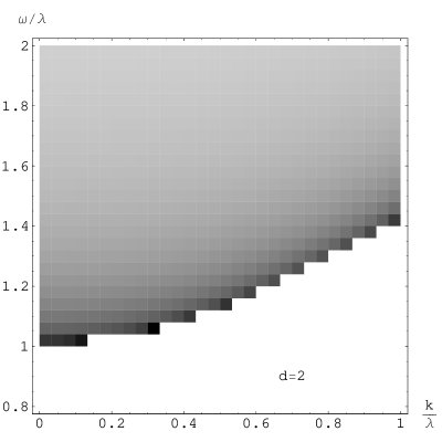
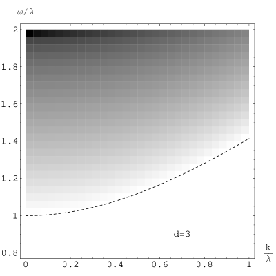
Figure 8: The imaginary part of the self energy in perturbation theory to order $g_{\psi}^{2}$. The upper plot is in two spatial dimensions; the lower plot is in three. In the lower plot, the dashed line is at $\omega^{2}=\lambda^{2}+k^{2}$.

VIII Critical properties: SSI–SSC (Class B2)

The transition between SSI and SSC is, as in Section VII, described by the (imaginary-time) action

$$\mathcal{S}_{\Psi}=\int\mathrm{d}^{d}\mathbf{x}\,\mathrm{d}\tau\>\left(|\partial\Psi|^{2}+r_{\Psi}|\Psi|^{2}+\frac{u_{\Psi}}{4}|\Psi|^{4}\right)\;\mathrm{,}$$ (112)

while the lowest-lying spin-carrying excitations now belong to the spin-$2$ field $d_{\mu\nu}$, with action

$$\mathcal{S}_{\Psi,d}=\int\mathrm{d}^{d}\mathbf{x}\,\mathrm{d}\tau\>\left[\bar{d}_{\mu\nu}\left(\partial_{\tau}-\frac{\nabla^{2}}{2m_{d}}+r_{d}\right)d_{\mu\nu}+g_{d}\bar{d}_{\mu\nu}d_{\mu\nu}\bar{\Psi}\Psi+\,\cdots\right]\;\mathrm{.}$$ (113)

As described in Section V.2.2, the dispersion is always irrelevant, while the coupling $g_{d}$ is marginal for $d=2$ and irrelevant above.

We therefore use perturbation theory in $g_{d}$ to describe the response function $\Pi_{Q}$. Since $\Pi_{Q}$ is related to the two-point correlator of $d_{\mu\nu}$ by Eq. (61), we are interested in self-energy diagrams for $d_{\mu\nu}$. Diagrams such as

$$\Sigma_{d}^{(0)}=\;\parbox{85.35826pt}{ \begin{picture}(30.0,15.0)\put(0.0,0.0){\includegraphics{fmfspindyn.23.ps}} \put(7.14854,5.39124){\makebox(0.0,0.0)[t]{$d_{\mu\nu}$}}\put(22.85146,5.39124){\makebox(0.0,0.0)[t]{$d_{\mu\nu}$}} \end{picture}}\;\mathrm{,}$$ (114)

which do not depend on the external momentum or frequency, simply renormalize the value of $r_{d}$ and are of no interest. The lowest-order diagram that we consider is therefore

$$\Sigma_{d}^{(1)}=\;\parbox{85.35826pt}{ \begin{picture}(30.0,20.0)\put(0.0,0.0){\includegraphics{fmfspindyn.24.ps}} \put(7.14854,5.39124){\makebox(0.0,0.0)[t]{$d_{\mu\nu}$}}\put(22.85146,5.39124){\makebox(0.0,0.0)[t]{$d_{\mu\nu}$}} \end{picture}}\;\mathrm{.}$$ (115)

Since $\Psi$ is critical, rather than using the free propagator $G^{\Psi}$ to describe this field, we use the full four-point (connected) correlation function, defined by

$$\Pi^{\Psi}(\mathbf{x},\tau)=\left\langle\mathcal{T}_{\tau}\>\bar{\Psi}(\mathbf{x},\tau)\Psi(\mathbf{x},\tau)\bar{\Psi}(\mathbf{0},0)\Psi(\mathbf{0},0)\right\rangle-\left\langle\bar{\Psi}(\mathbf{0},0)\Psi(\mathbf{0},0)\right\rangle^{2}\;\mathrm{.}$$ (116)

At the critical point, the Fourier transform of this correlation function has a power-law form, $\Pi^{\Psi}(\mathbf{k},\mathrm{i}\omega)=C(\sqrt{k^{2}+\omega^{2}})^{-y}$, where $C$ is a constant. The exponent $y$ is related to the scaling dimensions of the operator $|\Psi|^{2}$ at the critical point of $\mathcal{S}_{\Psi}$; the latter scaling dimension is $d+1-1/\nu$ (where $\nu$ is the correlation length exponent of the SSI to SSC transition), and so $y=2/\nu-d-1$. In $d=2$, the current best valuevicari is $\nu\approx 0.6717$, and so $y\approx-0.0225$. At leading order in $\epsilon$, a standard RG computation shows that $y=\frac{1}{5}\epsilon+\mathcal{O}\left(\epsilon^{2}\right)$. (Note that using this one-loop result corresponds to summing the diagram shown for $\Sigma_{d}^{(1)}$ as well as all ladder diagrams with increasing numbers of $u_{\Psi}$ interactions between the two $\Psi$ propagators.)

The self-energy diagram $\Sigma_{d}^{(1)}$ is then given by

$$\Sigma_{d}^{(1)}(\mathrm{i}\omega)=g_{d}^{2}\int_{\mathbf{k},\omega}G_{0}^{d}\biglb(\mathrm{i}(\omega+\nu)\bigrb)\Pi^{\Psi}(\mathbf{k},-\mathrm{i}\nu)\;\mathrm{,}$$ (117)

where the free propagator for $d_{\mu\nu}$ is given by

$$G_{0}^{d}(\mathrm{i}\omega)=\frac{1}{-\mathrm{i}\omega+r_{d}}\;\mathrm{.}$$ (118)

Using the explicit form of $\Pi^{\Psi}$, we have

$$\Sigma_{d}^{(1)}(\mathrm{i}\omega)=g_{d}^{2}C\int_{\mathbf{k}}\int_{-\infty}^{\infty}\frac{\mathrm{d}\nu}{2\pi}\frac{1}{-\mathrm{i}(\omega+\nu)+r_{d}}\cdot\frac{1}{(k^{2}+\nu^{2})^{y/2}}\;\mathrm{.}$$ (119)

The integrand is an analytic function apart from a pole at $\nu=-\omega-\mathrm{i}r_{d}$ and a branch cut along the imaginary axis for $\nu=\mathrm{i}x$, where $|x|>k$. Deforming the contour along the branch cut in the upper half-plane gives

$$\Sigma_{d}^{(1)}(\mathrm{i}\omega) =-\frac{g_{d}^{2}C}{\pi}\int_{\mathbf{k}}\int_{k}^{\infty}\mathrm{d}x\,\frac{1}{x-\mathrm{i}\omega+r_{d}}\operatorname{Im}\frac{1}{(k^{2}-x^{2})^{y/2}}$$ (120)

$$=-\frac{g_{d}^{2}C\sin(\pi y/2)}{\pi}\int_{\mathbf{k}}\int_{k}^{\infty}\mathrm{d}\xi\,\frac{1}{1+\xi+(r_{d}-\mathrm{i}\omega)/k}\cdot\frac{1}{[k^{2}\xi(1+2\xi)]^{y/2}}\;\mathrm{.}$$ (121)

Now consider the quasiparticle decay rate, found by analytically continuing $\mathrm{i}\omega$ to real frequencies and taking the imaginary part,

$$\operatorname{Im}\Sigma_{d}^{(1)}(r_{d}+\delta\omega)=-g_{d}^{2}C\sin(\pi y/2)\int_{\mathbf{k}}\frac{\Theta(\delta\omega-k)}{[(\delta\omega-k)(2\delta\omega-k)]^{y/2}}\;\mathrm{,}$$ (122)

where $\Theta$ is the unit-step function. The frequency can now be isolated from the integral, leaving

$$\operatorname{Im}\Sigma_{d}^{(1)}(r_{d}+\delta\omega)=-g_{d}^{2}C_{y}^{\prime}\delta\omega^{d-y}\;\mathrm{,}$$ (123)

where $C_{y}^{\prime}$ is a function of $y$ only.

Note that $d>y$, so that the decay rate, given by $\operatorname{Im}\Sigma_{d}$ evaluated at the quasiparticle energy, $\omega=r_{d}$, vanishes. This is as expected, since the spin-$2$ field $d_{\mu\nu}$ is, by assumption, the lowest-lying spin-carrying excitation. We therefore conclude that, contrary to the case described above in Section VII, the quasiparticle peak survives, even in the presence of gapless critical excitations of $\Psi$.

IX Conclusions

This paper has described a variety of representative models of spin dynamics across the superfluid insulator transition of spinful bosons. The main classes can be discussed in the context of the simple mean field phase diagram in Fig. 1 of $S=1$ bosons, with the three phases SSI (spin-singlet insulator), SSC (spin-singlet condensate) and PC (polar condensate).

First, we presented the spin response spectral functions in the three phases. The SSI and SSC phases have a spin gap, and consequently, the associated spin spectral density $A(\omega)$ has a non-zero value only above a threshold value given by the two $\psi_{\mu}$ particle continuum; the $\psi_{\mu}$ particle carries charge $Q=1$ and spin $F=1$. The nature of this threshold singularity was presented in Eq. (38) and below, and below Eq. (45) for the SSI phase. An alternative case, which could occur only well away from the PC phase, is that a $\psi_{\mu}$ particle and an anti-particle form a $Q=0$ bound state with non-zero spin, $d_{\mu\nu}$; in this case, the spin spectral function in the SSI phase consists of a sharp quasiparticle delta function at the spin gap energy. Closely related results apply to the SSC phase, as discussed in Section IV.3. Finally, for the PC phase, we have a gapless spin excitation, leading to Goldstone spin responses noted in Section IV.4.

Next, we described the quantum phase transitions between these phases under the following classes:
(A) This is the SSI to PC transition, associated with the condensation of the $\psi_{\mu}$. We found that the spin spectral density at the quantum critical point was determined by the scaling dimension of a composite spin operator which was bilinear in the $\psi_{\mu}$, as discussed in Section VI.
(B) This was the transition from the SSI to the SSC phase, driven by the condensation of $Q=2$, $F=0$ particle, $\Psi$. This class had two subclasses.
(B1) The lowest non-zero spin excitation consisted of the two-particle continuum of the $\psi_{\mu}$ particle. This was the most novel case, and was discussed at length in Section VII. Here we found interesting fluctuation corrections to the spin spectral density, characterized by the new ‘impurity’ exponent $\eta_{\Pi}$ in Eq. (99).
(B2) The spin response was associated with the sharp $Q=0$, $F=1$ quasiparticle $d_{\mu\nu}$, which can be stable well away from the PC phase. The damping of this quasiparticle from the critical $\Psi$ fluctuations was found to be associated with a composite operator whose scaling dimension was obtained in Section VIII. This damping led to powerlaw spectral absorption above the spin gap, but the quasiparticle peak survived even at the critical point.

In all of the above phases and quantum transitions we also obtained results for the nature of the single-particle Green’s function of the $\psi_{\mu}$ particle. This is not directly associated with a spin oscillation, because the $\psi_{\mu}$ particle has a non-zero charge $Q$. However, this can be measured experimentally in ‘photoemission’ type experiments, such as microwave absorption, which involve ejection of one boson from the atom trap.

We also did not consider the transition between the two superfluids in Fig. 1, the SSC and PC. This transition is associated with spin rotation symmetry breaking, and so has a charge neutral, vector O(3) order parameter. Consequently, the spin singularities can be mapped onto those of a relativistic O(3) model, which were described in much detail in Ref. csy, . However, here we also have to worry about the coupling of the critical O(3) modes to the gapless ‘phonon’ modes of the superfluids. The nature of this coupling was discussed in a different context in Ref. frey, , and it was found that as long as the free energy exponent $\alpha<0$, the coupling between the Goldstone and critical modes was irrelevant. It is known that this is the case for the O(3) model, and so the results of Ref. csy, apply unchanged to the SSC to PC transition.

We thank E. Demler, M. Lukin, R. Shankar, and E. Vicari for useful discussions. This research was supported by the NSF grants DMR-0537077, DMR-0342157, DMR-0354517, and PHY05-51164.

Appendix A Momentum cutoff RG

In Section VII, the scaling dimensions of the particle and hole excitations across the SSI–SSC transition were found using dimensional regularization. Here, we will peform the same calculation to one-loop order using a momentum cutoff. (The scaling dimension of the compound operator $p_{\mu}h_{\nu}$ can be found by an analogous calculation.)

Our approach will be to calculate the correlation functions of the gapped $p_{\mu}$ and $h_{\mu}$ excitations, evaluated for real frequencies just above the gap $\lambda$. (Imaginary frequencies will be used as a formal device when calculating the diagrams, followed by analytic continuation.) We will find that there is a rescaling operation that is a symmetry of the theory and relates correlation functions evaluated at one frequency to those evaluated at another, as in a standard RG calculation. In this case, however, it is necessary to rescale relative to the gap energy $\lambda$, rather than the zero of frequency.

A.1 Self-energy renormalization

As a result of particle conservation, there is no one-loop diagram contributing to the renormalization of the interaction vertex.

The only one-loop diagram for the self energy of the particle (or hole) excitation is given in Eq. (72):

$$\Sigma^{\psi}_{1}(\mathrm{i}\omega)=g_{\psi}^{2}\int_{\mathbf{k}}\int_{-\infty}^{\infty}\frac{\mathrm{d}\omega^{\prime}}{2\pi}\,G^{\Psi}_{0}(\mathbf{k},\mathrm{i}\omega^{\prime})G^{\psi}_{0}\biglb(\mathrm{i}(\omega-\omega^{\prime})\bigrb)\;\mathrm{,}$$ (124)

where

$$\int_{\mathbf{k}}\equiv\int\frac{\mathrm{d}^{d}\mathbf{k}}{(2\pi)^{d}}=\Omega_{d}\int_{0}^{\Lambda}\mathrm{d}k\,k^{d-1}$$ (125)

(for an isotropic integrand), with $\Lambda$ the cutoff. Since the dispersion of $p_{\mu}$ and $h_{\mu}$ is irrelevant, the diagram is calculated with the external momentum equal to zero.

Working at criticality, where we set $r_{\Psi}=0$, this gives

$$\Sigma^{\psi}_{1}(\mathrm{i}\omega)=g_{\psi}^{2}\int_{\mathbf{k}}\frac{1}{2k}\cdot\frac{1}{-\mathrm{i}\omega+\lambda+k}\;\mathrm{,}$$ (126)

after performing the integral over $\omega^{\prime}$ by contour integration. With the definition $z=-\mathrm{i}\omega+\lambda$, we have

$$\Sigma^{\psi}_{1}(\mathrm{i}\omega)=g_{\psi}^{2}\frac{\Omega_{d}}{2}\int_{0}^{\Lambda}\mathrm{d}k\,\frac{k^{d-2}}{k+z}\;\mathrm{.}$$ (127)

Using Dyson’s equation, the inverse of the propagator is therefore

$$G^{\psi}_{1}(\mathrm{i}\omega)^{-1}=z-\frac{g_{\psi}^{2}\Omega_{d}}{2}\int_{0}^{\Lambda}\mathrm{d}k\,\frac{k^{d-2}}{k+z}+\mathcal{O}\left(g_{\psi}^{4}\right)\;\mathrm{.}$$ (128)

Taking the derivative with respect to $\Lambda$ and expanding in powers of $z/\Lambda$ gives

$$\Lambda\frac{\partial G_{1}^{-1}}{\partial\Lambda}=-\frac{g_{\psi}^{2}\Omega_{d}}{2}\Lambda^{d-2}+\frac{g_{\psi}^{2}\Omega_{d}}{2}z\Lambda^{d-3}+\cdots\;\mathrm{.}$$ (129)

The first term is independent of $\omega$ and so corresponds to a renormalization of $\lambda$, which is of no interest to us. The second term corresponds to wavefunction renormalization and is the only relevant contribution from this diagram.

Since there is no diagram giving a renormalization of the coupling $g_{\psi}$, a reduction in the cutoff from $\Lambda$ to $(1-\delta)\Lambda$ (with $\delta$ infinitesimal) can be compensated by replacing the action $\mathcal{S}_{\Psi,\psi}$ by

$$\mathcal{S}_{\Psi,\psi}+\delta\mathcal{S}_{\Psi,\psi}=\int\mathrm{d}^{d}\mathbf{x}\,\mathrm{d}\tau\>\bigg{\{}\left(1+\hat{g}_{\psi}^{2}\delta\right)\left[\bar{p}_{\mu}\left(\partial_{\tau}+\lambda\right)p_{\mu}+\bar{h}_{\mu}\left(\partial_{\tau}+\lambda\right)h_{\mu}\right]\\ +g_{\psi}\left(\bar{\Psi}p_{\mu}\bar{h}_{\mu}+\Psi\bar{p}_{\mu}h_{\mu}\right)\bigg{\}}\;\mathrm{.}$$ (130)

To simplify this expression slightly, we have defined the dimensionless quantity $\hat{g}_{\psi}=g_{\psi}\Lambda^{-(d-3)/2}\sqrt{\Omega_{d}/2}$.

A.2 Partition function

This notion of ‘compensating a reduction in the cutoff’ can be made more precise by considering the partition function with discrete sources:

$$\mathcal{Z}_{\Lambda}(J_{i},\mathbf{k}_{i},z_{i},g_{\psi})=\int_{\Lambda}\mathcal{D}^{2}p\,\mathcal{D}^{2}h\>\exp-\bigg{\{}\int_{\omega,\mathbf{k}}(\bar{p}_{\mu}zp_{\mu}+\bar{h}_{\mu}zh_{\mu})\\ +g_{\psi}\int_{\omega_{1},\mathbf{k}_{1}}\int_{\omega_{2},\mathbf{k}_{2}}\left[\bar{\Psi}\biglb(\mathbf{k}_{1}-\mathbf{k}_{2},\mathrm{i}(\omega_{1}-\omega_{2})\bigrb)p_{\mu}(\mathbf{k}_{1},\mathrm{i}\omega_{1})\bar{h}_{\mu}(\mathbf{k}_{2},\mathrm{i}\omega_{2})+\mathrm{c.c.}\right]\\ +\sum_{i}\bar{J}_{i\mu}[p_{\mu}(\mathbf{k}_{i},\lambda-z_{i})+\bar{h}_{\mu}(\mathbf{k}_{i},\lambda-z_{i})]+\mathrm{c.c.}\bigg{\}}\;\mathrm{,}$$ (131)

from which correlation functions can be found by successive differentiation with respect to $J_{i}$ and $\bar{J}_{i}$. (We are concerned with $\psi_{\mu}$, so integration over $\Psi$, with the appropriate measure, is implied.) The subscript $\Lambda$ on the integral sign denotes that a cutoff $\Lambda$ should be used.

Using this definition, Eq. (130) can be written

$$\mathcal{Z}_{\Lambda}(J_{i},z_{i},g_{\psi})=\int_{(1-\delta)\Lambda}\mathcal{D}^{2}p\,\mathcal{D}^{2}h\>\exp-\bigg{\{}\left(1+\hat{g}_{\psi}^{2}\delta\right)\int_{\omega,\mathbf{k}}(\bar{p}_{\mu}zp_{\mu}+\bar{h}_{\mu}zh_{\mu})\\ +g_{\psi}\int\!\!\!\!\int_{\omega,\mathbf{k}}\left(\bar{\Psi}p_{\mu}\bar{h}_{\mu}+\mathrm{c.c.}\right)+\sum_{i}\bar{J}_{i\mu}[p_{\mu}(\lambda-z_{i})+\bar{h}_{\mu}(\lambda-z_{i})]+\mathrm{c.c.}\bigg{\}}\;\mathrm{,}$$ (132)

which expresses the fact that the partition function, and hence all correlators, are unchanged by a shift in the cutoff and a compensating change in the action. A condensed notation has been used, where the momentum dependence is suppressed throughout.

To bring this closer to the form of Eq. (131), we rescale the fields $p_{\mu}$ and $h_{\mu}$ within the functional integral. By doing so, we can return the coefficient of the quadratic term to unity, giving

$$\mathcal{Z}_{\Lambda}(J_{i},z_{i},g_{\psi})=\int_{(1-\delta)\Lambda}\mathcal{D}^{2}p\,\mathcal{D}^{2}h\>\exp-\bigg{\{}\int_{\omega,\mathbf{k}}(\bar{p}_{\mu}zp_{\mu}+\bar{h}_{\mu}zh_{\mu})\\ +g_{\psi}\left(1-\hat{g}_{\psi}^{2}\delta\right)\int\!\!\!\!\int_{\omega,\mathbf{k}}\left(\bar{\Psi}p_{\mu}\bar{h}_{\mu}+\mathrm{c.c.}\right)\\ +\sum_{i}\left(1-\frac{\hat{g}_{\psi}^{2}}{2}\delta\right)J_{i\mu}[p_{\mu}(\lambda-z_{i})+\bar{h}_{\mu}(\lambda-z_{i})]+\mathrm{c.c.}\bigg{\}}\;\mathrm{.}$$ (133)

By comparison with Eq. (131), we can write

$$\mathcal{Z}_{\Lambda}(J_{i},\mathbf{k}_{i},z_{i},g_{\psi})=\mathcal{Z}_{(1-\delta)\Lambda}\biglb(\left(1-\hat{g}_{\psi}^{2}\delta/2\right)J_{i},\mathbf{k}_{i},z_{i},\left(1-\hat{g}_{\psi}^{2}\delta\right)g_{\psi}\bigrb)\;\mathrm{.}$$ (134)

A.3 Rescaling

To return to the original theory, with cutoff $\Lambda$, we now perform a rescaling of all variables according to their engineering dimensions, with $[\tau]=[\mathbf{x}]=-1$. Since we are working at the critical point of $\Psi$, we have

$$\Psi(\mathbf{x}/b,\tau/b)=b^{X}\Psi(\mathbf{x},\tau)\;\mathrm{,}$$ (135)

where $X$ is the scaling dimension of the field $\Psi$. By dimensional analysis of Eq. (68), the engineering dimension of $\Psi$ is seen to be $[\Psi]=(D-2)/2=(d-1)/2$ and one would naively expect $X=[\Psi]=1-\frac{\epsilon}{2}$. This expectation actually happens to be correct (to order $\epsilon$), since there is no wavefunction renormalization of $\mathcal{S}_{\Psi}$ to one-loop order.

Performing this rescaling leads to

$$\mathcal{Z}_{\Lambda}(J_{i},\mathbf{k}_{i},z_{i},g_{\psi})=\mathcal{Z}_{b\Lambda}(b^{1+d/2}J_{i},b\mathbf{k}_{i},bz_{i},b^{1-X}g_{\psi})\;\mathrm{,}$$ (136)

after making the substitutions $\psi^{\prime}(\mathbf{k},\lambda-z)=b^{d/2+1}\psi(b\mathbf{k},\lambda-bz)$ and $\lambda-\mathrm{i}\omega^{\prime}=(\lambda-\mathrm{i}\omega)/b$.

This can now be combined with Eq. (134) to give

$$\mathcal{Z}_{\Lambda}(J_{i},\mathbf{k}_{i},z_{i},g_{\psi})=\mathcal{Z}_{\Lambda}\biglb((1-\hat{g}_{\psi}^{2}\delta/2)(1+(1+d/2)\delta)J_{i},(1+\delta)\mathbf{k}_{i},(1+\delta)z_{i},\\ (1-\hat{g}_{\psi}^{2}\delta)(1+(1-X)\delta)g_{\psi}\bigrb)\;\mathrm{.}$$ (137)

This gives a relationship between correlators in the same theory but at different frequencies.

The fixed point of Eq. (137) occurs when

$$g_{\psi}^{\star}=[1-(\hat{g}_{\psi}^{\star})^{2}\delta][1+(1-X)\delta]g_{\psi}^{\star}\;\mathrm{,}$$ (138)

so that

$$\hat{g}_{\psi}^{\star}=\sqrt{1-X}=\sqrt{\frac{\epsilon}{2}}\;\mathrm{,}$$ (139)

which should be compared with Eq. (87).

A.4 Renormalized propagator

At the fixed point, Eq. (137) becomes

$$\mathcal{Z}_{\Lambda}(J_{i},\mathbf{k}_{i},z_{i},g_{\psi}^{\star})=\mathcal{Z}_{\Lambda}\biglb((1+y\delta)J_{i},(1+\delta)\mathbf{k}_{i},(1+\delta)z_{i},g_{\psi}^{\star}\bigrb)\;\mathrm{,}$$ (140)

where $y=1+d/2-(\hat{g}_{\psi}^{\star})^{2}/2=5/2-3\epsilon/4$. Taking derivatives with respect to $J_{\mu}$ and $\bar{J}_{\nu}$ gives

$$\left\langle\bar{\psi}_{\mu}(\mathbf{k}_{1},\lambda-z_{1})\psi_{\nu}(\mathbf{k}_{2},\lambda-z_{2})\right\rangle=\\ (1+2y\delta)\big{\langle}\bar{\psi}_{\mu}\biglb((1+\delta)\mathbf{k}_{1},\lambda-(1+\delta)z_{1}\bigrb)\psi_{\nu}\biglb((1+\delta)\mathbf{k}_{2},\lambda-(1+\delta)z_{2}\bigrb)\big{\rangle}\;\mathrm{.}$$ (141)

Using the conservation of frequency and momentum, we can define the propagator $G^{\psi}$ by

$$\left\langle\bar{\psi}_{\mu}(\mathbf{k}_{1},\lambda-z_{1})\psi_{\nu}(\mathbf{k}_{2},\lambda-z_{2})\right\rangle=(2\pi)^{d+1}\delta^{d}(\mathbf{k}_{1}-\mathbf{k}_{2})\delta(z_{1}-z_{2})\delta_{\mu\nu}G^{\psi}(\mathbf{k}_{1},\lambda-z_{1})\;\mathrm{.}$$ (142)

Using this definition, Eq. (141) becomes

$$G^{\psi}(\mathbf{k},\lambda-z)=(1+y^{\prime}\delta)G^{\psi}\biglb((1+\delta)\mathbf{k},\lambda-(1+\delta)z\bigrb)\;\mathrm{,}$$ (143)

with $y^{\prime}=2y-d-1=1-\epsilon/2$.

Restricting attention to $\mathbf{k}=\mathbf{0}$ gives

$$G^{\psi}(\mathbf{0},\lambda-z)=(1+y^{\prime}\delta)G^{\psi}\biglb(\mathbf{0},\lambda-(1+\delta)z\bigrb)\;\mathrm{,}$$ (144)

which can be iterated to give

$$G^{\psi}(\mathbf{0},\lambda-z)\sim z^{-1+\epsilon/2}\;\mathrm{.}$$ (145)

Equivalently, after analytic continuation to real frequencies, we have

$$G^{\psi}(\mathbf{0},\omega)\sim(\lambda-\omega)^{-1+\epsilon/2}\;\mathrm{,}$$ (146)

which agrees with Eq. (89).

References

- (1) J. Stenger, S. Inouye, D. M. Stamper-Kurn, H. J. Miesner, A. P. Chikkatur, and W. Ketterle, Nature 396, 345 (1998).
- (2) M. S. Chang, C. D. Hamley, M. D. Barrett, J. A. Sauer, K. M. Fortier, W. Zhang, L. You, and M. S. Chapman, Phys. Rev. Lett. 92, 140403 (2004).
- (3) J. M. Higbie, L. E. Sadler, S. Inouye, A. P. Chikkatur, S. R. Leslie, K. L. Moore, V. Savalli, and D. M. Stamper-Kurn, Phys. Rev. Lett. 95, 050401 (2005).
- (4) M. S. Chang, Q. S. Qin, W. X. Zhang, L. You, and M. S. Chapman, Nature Phys. 1, 111 (2005).
- (5) J. Mur-Petit, M. Guilleumas, A. Polls, A. Sanpera, M. Lewenstein, K. Bongs, and K. Sengstock, Phys. Rev. A 73, 013629 (2006).
- (6) J. Kronjäger, C. Becker, M. Brinkmann, R. Walser, P. Navez, K. Bongs, and K. Sengstock, cond-mat/0509083.
- (7) A. Widera, F. Gerbier, S. Fölling, T. Gericke, O. Mandel, and I. Bloch, Phys. Rev. Lett. 95, 190405 (2005)
- (8) F. Gerbier, A. Widera, S. Fölling, O. Mandel, and I. Bloch, Phys. Rev. A 73, 041602 (2006).
- (9) H.-J. Huang and G.-M. Zhang, cond-mat/0601188.
- (10) A. Imambekov, M. Lukin, and E. Demler, Phys. Rev. A 68, 063602 (2003).
- (11) S. Tsuchiya, S. Kurihara, and T. Kimura, Phys. Rev. A 70, 043628 (2004).
- (12) D. Rossini, M. Rizzi, G. De Chiara, S. Montangero, and R. Fazio, J. Phys. B: At. Mol. Opt. Phys. 39, S163 (2006).
- (13) L. Zawitkowski, K. Eckert, A. Sanpera, and M. Lewenstein, cond-mat/0603273.
- (14) S. Sachdev, M. Troyer, and M. Vojta, Phys. Rev. Lett. 86, 2617 (2001).
- (15) S. Sachdev, Physica C 357, 78 (2001).
- (16) S. Powell and S. Sachdev, Phys. Rev. A in press, cond-mat/0608611
- (17) R. Barnett, A. Turner, and E. Demler, cond-mat/0607253.
- (18) M. Lewenstein, A. Sanpera, V. Ahufinger, B. Damski, A. Sen De, U. Sen, cond-mat/0606771 (unpublished).
- (19) S. Sachdev, Quantum Phase Transitions, Cambridge University Press, Cambridge (1999).
- (20) M. P. A. Fisher, P. B. Weichman, G. Grinstein, and D. S. Fisher, Phys. Rev. B 40, 546 (1989).
- (21) E. Demler, and F. Zhou, Phys. Rev. Lett. 88. 163001 (2002).
- (22) S. Tsuchiya. S. Kurihara, and T. Kimura, Phys. Rev. A 70, 043628 (2004).
- (23) V. N. Popov, Functional Integrals and Collective Excitations, Cambridge University Press, Cambridge (1988).
- (24) M. De Prato, A. Pelissetto, and E. Vicari, Phys. Rev. B 70, 214519 (2004).
- (25) P. Calabrese, A. Pelissetto, and E. Vicari, Nucl. Phys. B 709, 550 (2005).
- (26) J. Zinn-Justin, Quantum Field Theory and Critical Phenomena, Oxford University Press, Oxford (1996).
- (27) M. Campostrini, M. Hasenbusch, A. Pelissetto, and E. Vicari, Phys. Rev. B 74, 144506 (2006).
- (28) A. V. Chubukov, S. Sachdev, and J. Ye, Phys. Rev. B 49, 11919 (1994).
- (29) E. Frey and L. Balents, Phys. Rev. B 55, 1050 (1997).