Driven dissipative dynamics of spins in quantum dots

Abstract

We have studied the dissipative dynamics of a driven electronic spin trapped in a quantum dot. We consider the dissipative mechanism as due to the indirect coupling of the electronic spin to acoustic phonons via the spin-orbit/electron-phonon couplings. Using an effective spectral function of the dissipative phonon bath, we evaluated the expectation values of the spin components through the Bloch-Redfield theory. We show that due to a sharp bath resonance present in the effective spectral function, with typical energy much smaller than the electronic confinement energy, the dissipative spin has a rich dynamical behavior that helps us to determine some features of the spin-bath coupling. We also quantify the effects produced by the sharp bath resonance, and thus indicate the best regimes of operation in order to achieve the longest relaxation times for the spin.

I Introduction

During the last decade several physical systems have been proposed as candidates for qubits nielsen and, among those, condensed matter devices have been attracting a growing interest in the area guido . There are many reasons for this and most of them involve the way one designs, controls and accesses individual qubits in quantum systems containing a very large number of such entities. This is a natural consequence of the fact that dealing with solid state devices one can use the same standard electronic circuitry of conventional computers. Furthermore, new and powerful experimental techniques allow us to expect that these qubits could be more easily scalable and that control over the processing of information and implementation of possible protocols of error correction could be done in a more reliable and efficient way. These are only a few points in favour of these systems as being good candidates for qubits.

Despite these important favourable points, there are also negative aspects concerning the use of solid state devices as qubits. Since they are mainly meso or nanoscopic devices, which under specific conditions mimic two-state system behavior, it is a very hard task to isolate them from their environment. Moreover, as it is already well known, the system-bath interaction causes loss of quantum coherence which is a drawback for quantum computation CL ; leggett , in particular, if we do not wish to operate our devices at too low temperatures. Therefore, there must be a compromise between the desirable features possessed by these systems and the undesirable effect of decoherence. It is along this direction that people have been investigating electronic spins in quantum dots as promising candidates for qubits lossdavid ; gld . Since the confinement of the electronic wave function isolates the spins from most energy relaxation channels, there are situations where decoherence takes place only beyond a fairly long time interval. Here we mean a time interval within which a large number of logical operations could be coherently performed. In particular, for self-assembled quantum dots, the energies involved in the spin dynamics are such that the decoherence time is indeed very long. However, what is advantageous on the one hand turns out to be a problem otherwise. As the spin is a microscopic variable one has to face the problem of how to access it experimentally.

A possible way to address one of the many spins in the quantum processor is by tuning the frequency of a time dependent external magnetic field (the transverse pumping or control field) to the spin’s Larmor frequency. Indeed, Koppens and collaborators Koppens have demonstrated very recently the first experimental realization of single electron spin rotations in quantum dot systems, which is a necessary step for the implementation of universal quantum operations. They showed, through current measurements in double quantum dots, the ability of performing spin-flips using a resonant oscillating magnetic field with the spin’s Larmor frequency. Therefore, in this work, we shall investigate the dissipative dynamics of an electronic spin confined to a quantum dot subject to a strong static magnetic field and a much weaker transverse pumping field.

It has been demonstrated that the main mechanisms of relaxation of the latter are the spin-orbit interaction alexander ; ivchenko and the hyperfine interaction with the spins of the host lattice erlingsson . For static fields stronger than $1$T it is expected that the spin-orbit interaction plays a major role in the relaxation process. The relaxation times experimentally observed for fields above $4$T are within the range $\sim 0.8-20$mskroutvar ; elzerman which encourages us to study the possibility of implementing spins confined in quantum dots as qubits.

Following previous works harry , we investigate the dissipative effects originating from the coupling of the orbital electronic motion to the acoustic phonon modes of the lattice where the dots are embedded. Due to the spin-orbit coupling, the spin degree of freedom becomes indirectly damped by the latter. Consequently, it is possible to define an effective dissipative two-state system harry whose dynamics may not be describable pertubatively khaetskii . In particular, one should stress the existence of a very sharp effective bath resonance at energies much lower than the planar electronic confinement energy.

The main goal of the present work is to evaluate the dissipative dynamics of a structured spin-boson model in the presence of a time dependent magnetic field aiming at the determination of the best operational conditions under which these systems could be employed as good qubits. In section II we present the model we use to describe this dynamical process. In section III, we obtain the approximate analytical solutions to the Bloch-Redfield equations for the average values of the spin components. Finally, in section IV, we carry out a detailed analysis of the solutions we have obtained.

II Model

We consider quantum dots with strong confinement in the $z$ direction, and electronic orbital motion in the $x-y$ plane subject to a confining parabolic potential. The spin-orbit coupling is modelled by a Dresselhaus interaction term projected onto the plane of the dot. Besides, we add a term due the presence of an externally applied magnetic field $\bf B$. Thus, these assumptions lead to the following spin-orbit Hamiltonian

$$H_{SO} = \hbar\omega_{0}\left(a_{x}^{\dagger}a_{x}+\frac{1}{2}\right)-\beta\hat{\sigma}_{x}P_{x}$$ (1)

$$+\hbar\omega_{0}\left(a_{y}^{\dagger}a_{y}+\frac{1}{2}\right)+\beta\hat{\sigma}_{y}P_{y}+\frac{1}{2}g\mu_{B}{\bf{B}}\cdot{\boldsymbol{\hat{\sigma}}},\quad$$

where $\omega_{0}$ is the lateral harmonic frequency, $\beta\equiv\gamma_{c}\langle k_{z}^{2}\rangle=\gamma_{c}m^{\ast}\omega_{\bot}$ (with $\gamma_{c}$ is the Kane parameterivchenko , $m^{\ast}$ is the electron effective mass), $\hat{\boldsymbol{\sigma}}$ are the Pauli matrices, and $a_{x(y)}$ is the usual ladder operators for the $x(y)$ direction.

The electron-phonon Hamiltonian, considering either the piezoelectric or the deformation potential interactions with acoustic phonon modes, can be mapped into the bath of oscillators model CL with the spectral function given by harry

$$J_{s}\left(\omega\right)=m^{\ast}\omega_{D}^{2}\delta_{s}\left(\frac{\omega}{\omega_{D}}\right)^{s}\theta\left(\omega_{D}-\omega\right),$$ (2)

where $s=3$ for the piezoelectric interaction with dimensionless coupling $\delta_{3}=\frac{(e_{m})_{14}^{2}\omega_{D}}{35\pi m^{\ast}\rho}\left(\frac{4}{3v_{t}^{5}}+\frac{1}{v_{l}^{5}}\right)$, and $s=5$ for the deformation potential with $\delta_{5}=\frac{a_{c\Gamma}^{2}\omega_{D}^{3}}{2\pi\rho m^{\ast}v_{l}^{7}}$, where $\omega_{D}$ is the Debye frequency. $v_{l}$ and $v_{t}$ are the longitudinal and transverse sound velocities respectively, $\rho$ is the material density, $(e_{m})_{14}$ is the electromechanical tensor for zinc-blende structurescardona , and $a_{c,\Gamma}$ is the deformation potential at the $\Gamma$ pointcardona . $\theta$ is the Heaviside step function.

Provided that we have introduced a bath of oscillators for the electron-phonon coupling, and because of the spin-orbit interaction, one can think of this problem as a spin degree of freedom coupled to an effective bath of oscillators harry with the following effective bath spectral function

$$J_{eff}\left(\omega\right)=m^{\ast}\beta^{2}\frac{\delta_{s}\left(\frac{\omega}{\omega_{D}}\right)^{s+2}}{Z\left(\omega\right)^{2}+\delta_{s}^{2}\left(\frac{\omega}{\omega_{D}}\right)^{2s}}\theta\left(\omega_{D}-\omega\right),$$ (3)

where $Z\left(\omega\right)\equiv\left(\frac{\omega_{0}}{\omega_{D}}\right)^{2}-\left(\frac{\omega}{\omega_{D}}\right)^{2}\left(1+\delta_{s}\phi_{s}\left(\frac{\omega}{\omega_{D}}\right)\right)$, and $\phi_{s}(x)\equiv\frac{2}{\pi}P\int_{0}^{1}x^{s}/(y^{3}-yx^{2})dy=-\frac{x^{s-2}}{\pi}(B(x,s,0)+(-1)^{s}B(-x,s,0))$, with $B$ being the generalized incomplete beta function.

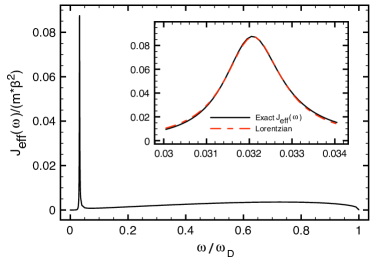
Figure 1: Spectral density $J_{eff}$ for piezoelectric electron-phonon interaction, $s=3$. Inset: The region close to the peak $\Omega_{s}$ can be well approximated by the Lorentzian in Eq. 5 (dashed line). Here we assumed $\frac{\omega_{0}}{\omega_{D}}\approx 0.5$ and $\delta_{3}=355$.

Figure 1 presents the $J_{eff}(\omega)$ behavior for the piezoelectric interaction case, $s=3$. The most prominent feature of its behavior is the peak at $\omega=\Omega_{s}$, where $\Omega_{s}$ is determined by

$$\Omega_{s}\approx\omega_{0}\sqrt{\frac{(s-2)}{(s-2)+\frac{2\delta_{s}}{\pi}}}.$$ (4)

Furthermore, the region around $\Omega_{s}$ can be well approximated by a Lorentzian of width $\ell\approx\frac{\omega_{D}\pi(s-2)}{4}\left(\frac{\omega_{0}}{\omega_{D}}\sqrt{\frac{(s-2)\pi}{2\delta_{s}}}\right)^{s-1}$ (see inset of Figure 1), given by

$$J_{eff}(\omega\approx\Omega_{s})\approx\frac{m^{\ast}\beta^{2}}{2}\left(\frac{\omega_{D}}{\omega_{0}}\right)^{2}\frac{\Omega_{s}^{3}}{\omega_{D}}\left(\frac{\ell}{(\omega-\Omega_{s})^{2}+\ell^{2}}\right).$$ (5)

The asymptotic analysis of $J_{eff}(\omega)$ also reveals that in the low frequency range, defined by $\omega\ll\Omega_{s}$ and $\frac{\omega}{\omega_{D}}\ll\left(\frac{\omega_{0}}{\omega_{D}}\frac{1}{\delta_{s}}\right)^{1/s}$, the effective spectral density is always super-ohmic, with power $s+2$. On the opposite side of the resonance, and in the high frequency limit, $\Omega_{s}\ll\omega\ll\omega_{D}$, the spectral density behaves as a power law in the frequency $\omega$ with exponent $s-2$.

Since we know the spectral density of the effective bath of oscillators coupled to the spin degree of freedom, our problem can now be modelled by the driven spin-boson Hamiltonian

$$H\left(t\right) = -\frac{\hbar}{2}[\Delta\hat{\sigma}_{x}+\epsilon\left(t\right)\,\hat{\sigma}_{z}]$$ (6)

$$+\sum_{i}\hbar\omega_{i}\left(\hat{b}_{i}^{\dagger}\hat{b}_{i}+\frac{1}{2}\right)+\hat{\sigma}_{z}\sum_{i}c_{i}\left(\hat{b}_{i}^{\dagger}+\hat{b}_{i}\right),\quad$$

where the spectral density of the environment is given by (3), and the applied magnetic field ${\bf B}=(-\hbar\Delta/g\mu_{B},0,-\hbar\epsilon(t)/g\mu_{B})$. In the weak coupling limit, the equations of motion for the spin expectation values, $\sigma_{i}\left(t\right)\equiv Tr\left[\hat{\rho}\left(t\right)\hat{\sigma}_{i}\right]$, can be written, for this specific model, as the generalized Bloch-Redfield equation hartmann

$$\dot{\sigma}_{x}\left(t\right)\!\!\! = \!\epsilon\left(t\right)\sigma_{y}-\Gamma_{xx}\left(t\right)\sigma_{x}-\Gamma_{xz}\left(t\right)\sigma_{z}-A_{x}\left(t\right),$$

$$\dot{\sigma}_{y}\left(t\right)\!\!\! = \!-\epsilon\left(t\right)\sigma_{x}+\Delta\sigma_{z}-\Gamma_{yy}\left(t\right)\sigma_{y}-\Gamma_{yz}\left(t\right)\sigma_{z}-A_{y}\left(t\right),$$

$$\dot{\sigma}_{z}\left(t\right)\!\!\! = \!-\Delta\sigma_{y},$$ (7)

where the fluctuating terms are given by hartmann

$$A_{x}\left(t\right)=\textrm{Im}F\left(t\right),\leavevmode\nobreak\ A_{y}\left(t\right)=\textrm{Re}F\left(t\right),\leavevmode\nobreak\ {\rm with}$$

$$F\left(t\right)=2\int_{0}^{t}dt^{\prime}\textrm{Im}M(t-t^{\prime})\,U_{RR}(t,t^{\prime})U_{RL}(t,t^{\prime}),$$

and the temperature dependent relaxation rates are determined byhartmann

$$\Gamma_{ij}\left(t\right)=\int_{0}^{t}dt^{\prime}\textrm{Re}[M(t-t^{\prime})]b_{ij}(t,t^{\prime}),\leavevmode\nobreak\ {\rm with}\leavevmode\nobreak\ \Gamma_{yy}\left(t\right)=\Gamma_{xx}\left(t\right).$$

The correlation function

$$M\left(t\right)=\frac{1}{\pi}\int_{0}^{\infty}d\omega J(\omega)\frac{\cosh(\frac{\beta\omega}{2}-i\omega t)}{\sinh(\frac{\beta\omega}{2})},$$

with $\beta\equiv 1/k_{B}T$, takes into account all the effects of the bath of oscillators. The functions $b_{ij}$ read

$$b_{xz}=2\textrm{Re}\left[U_{RR}U_{RL}\right],\leavevmode\nobreak\ b_{yz}=-2\textrm{Im}\left[U_{RR}U_{RL}\right]$$

and $b_{xx}=|U_{RR}|^{2}-|U_{RL}|^{2},$ where $U(t,t^{\prime})$ is the non-dissipative time evolution operator for the spin system and its matrix elements $U_{RR}(t,t^{\prime})=\langle R|U(t,t^{\prime})|R\rangle$ and $U_{RL}(t,t^{\prime})=\langle R|U(t,t^{\prime})|L\rangle$, are written in the basis defined by $\sigma_{z}|R\rangle\equiv+|R\rangle,\sigma_{z}|L\rangle\equiv-|L\rangle$. Eqs. (7) are derived hartmann under the assumption that $\frac{J(\omega)}{\omega}\ln(\Omega_{c}/\Delta)\ll 1$, where $\Omega_{c}$ represents the cutoff frequency of the system.

III Results

From here onwards we will be interested in the study of a monochromatic field of the form $\epsilon\left(t\right)=2\epsilon_{0}\cos\Omega t$, considering it as a small perturbation to the spin dynamics, i.e., $\epsilon_{0}/\Delta\ll 1$. In order to solve the Bloch-Redfield equations we need to compute the non-dissipative time evolution operator $U(t,t^{\prime})$. Using the rotating wave approximation (RWA), we obtain the following simple analytic form to the time evolution operator

$$U(t,t_{0})=R_{x}^{\dagger}\left(\Omega t\right)e^{\frac{i}{2}\epsilon_{1}(t-t_{0})\hat{\boldsymbol{\sigma}}\cdot\mathbf{n}}R_{x}(\Omega t_{0}),$$ (8)

where $R_{x}\left(\Omega t\right)=e^{-\frac{i}{2}\Omega t\hat{\sigma}_{x}}$, $\hat{\boldsymbol{\sigma}}\cdot\mathbf{n}=\frac{\Delta-\Omega}{\epsilon_{1}}\hat{\sigma}_{x}+\frac{\epsilon_{0}}{\epsilon_{1}}\hat{\sigma}_{z}=\cos\left(\phi\right)\hat{\sigma}_{z}+\sin\left(\phi\right)\hat{\sigma}_{x}$, with $\tan\left(\phi\right)\equiv\frac{\Delta-\Omega}{\epsilon_{0}}$ and $\epsilon_{1}\equiv\sqrt{\epsilon_{0}^{2}+\left(\Delta-\Omega\right)^{2}}$. $\epsilon_{1}$ and $\Delta$ are, respectively, the Rabi and Larmor frequencies of the problem, $\Omega$ is the external field frequency and $\phi$ represents the frequency detuning. The Bloch-Redfield coefficients can now be evaluated using the spectral density of the bath oscillators and $U\left(t,t^{\prime}\right)$. We proceed evaluating the time integrals first. Those have sine and co-sine elementary integrands that, when appropriately rearranged, can be written in terms of $sinc$ functions, whose maxima occur at the natural frequencies of the system $\Omega$, and $\Omega\pm\epsilon_{1}$. Following this procedure, the coefficients of the Bloch-Redfield equations can be written in the compact form

$$A_{x}\left(t\right) = r_{1}\left(t\right)+m_{1}\left(t\right)\sin\left(2\Omega t\right)+n_{1}\left(t\right)\cos\left(2\Omega t\right),$$

$$A_{y}\left(t\right) = m_{2}\left(t\right)\sin\left(\Omega t\right)+n_{2}\left(t\right)\cos\left(\Omega t\right),$$

$$\Gamma_{xx}\left(t\right) = r_{3}\left(t\right)+m_{3}\left(t\right)\sin\left(2\Omega t\right)+n_{3}\left(t\right)\cos\left(2\Omega t\right),$$ (9)

$$\Gamma_{xz}\left(t\right) = m_{4}\left(t\right)\sin\left(\Omega t\right)+n_{4}\left(t\right)\cos\left(\Omega t\right),$$

$$\Gamma_{yz}\left(t\right) = r_{5}\left(t\right)+m_{5}\left(t\right)\sin\left(2\Omega t\right)+n_{5}\left(t\right)\cos\left(2\Omega t\right),$$

(see appendix for the explicit presentation of those coefficients). The new coefficients $r_{i}\left(t\right),\,m_{i}\left(t\right)$ and $n_{i}\left(t\right)$ have their time dependence determined by the integrals $I_{n}$, Eqs. (19) and (20). Those integrals, in the regime of interest, $t\gg 1/\omega_{D}$, have their main contributions decomposed in two parts: one, time-dependent, occurs due to terms arising from the poles of the spectral density in the complex plane, which have lifetimes determined by their imaginary parts; the other part is a time-independent contribution due to the resonance of system with the external applied field. Therefore, each coefficient $r_{i}\left(t\right),\,m_{i}\left(t\right)$ and $n_{i}\left(t\right)$ can also be written in well-characterized time dependent and independent parts. In fact, considering $J(\omega)$ given by (3), whose main poles are $\Omega_{s}\pm i\ell$, we can write $r_{1}(t)$ as

$$r_{1}\left(t\right) \approx \ell J\left(\Omega_{s}\right)e^{-\ell t}\sum_{i=0}^{2}C_{i}\Bigg{\{}\frac{\sin\left[\left(\Omega_{s}-\Omega^{(i)}\right)t\right]}{\Omega_{s}-\Omega^{(i)}}$$ (10)

$$+\frac{\sin\left[\left(\Omega_{s}+\Omega^{(i)}\right)t\right]}{\Omega_{s}+\Omega^{(i)}}\Bigg{\}}+\tilde{r}_{1},$$

where $\Omega^{(0)}\equiv\Omega,\,\,\Omega^{(1)}\equiv\Omega+\epsilon_{1}\quad\text{and}\quad\Omega^{(2)}\equiv\Omega-\epsilon_{1}$; $C_{0}\equiv\cos\left(\phi\right)^{2}/2,\,\,C_{1}\equiv\left(1+\sin(\phi)\right)^{2}/4,\,\rm{and}\leavevmode\nobreak\ C_{2}\equiv\left(1-\sin(\phi)\right)^{2}/4$. The first term on the r.h.s of Eq. (10) is a direct contribution of the poles of $J\left(\omega\right)$ , and the last term, $\tilde{r}_{1}$, takes into account the time independent terms of $r_{1}\left(t\right)$. Substituting (10) in the Bloch-Redfield equations, we can find a particular solution for $\sigma_{x}$, up to first order in $\ell$, due to the first term of Eq. (10). Thus we can write $\sigma_{x}\left(t\right)$ as follows

$$\sigma_{x}\left(t\right) \approx \ell J\left(\Omega_{s}\right)e^{-\ell t}\sum_{i=0}^{2}C_{i}\Bigg{\{}\frac{\left(1-\cos\left(\Omega_{s}-\Omega^{(i)}\right)t\right)}{\left(\Omega_{s}-\Omega^{(i)}\right)^{2}}$$

$$+\frac{\left(1-\cos\left(\Omega_{s}+\Omega^{(i)}\right)t\right)}{\left(\Omega_{s}+\Omega^{(i)}\right)^{2}}\Bigg{\}}+\tilde{\sigma}_{x}\left(t\right).$$

It is clear that the particular solution has a lifetime determined by the width $\ell$ of the peak of the effective spectral density. The modes arising from this term oscillate with the system’s natural frequencies shifted by the bath resonance $\Omega_{s}$. Thus, the contributions due to the poles of $J_{eff}(\omega)$ introduce a new time scale, $1/\ell$, in the dynamics of the dissipative spin, which distinguishes the short and long time regimes of the problem. The first term of (10) is expected to be the dominant contribution of the poles of $J_{eff}(\omega)$ for the spin dynamics, because those arising from $m_{1}(t)$ and $n_{1}(t)$ oscillate with frequency $2\Omega$ larger than those from $r_{1}(t)$. After integrating the equations of motion over any measurable time interval, their effects become negligible.

Now, since we have determined the coefficients $r(t),\leavevmode\nobreak\ m(t),\leavevmode\nobreak\ {\rm{and}}\leavevmode\nobreak\ n(t)$, we can obtain analytic solutions for the Bloch-Redfield equations. For the long time regime, $t>1/\ell$, those coefficients approach very quickly their asymptotic values $\tilde{f}\equiv f(t\rightarrow\infty)$, with $f=r,\leavevmode\nobreak\ m,\leavevmode\nobreak\ {\rm{and}}\leavevmode\nobreak\ n$. A solution can be obtained using the Laplace transformation for the regime of interest, namely $\epsilon_{0}/\Delta\ll 1$. Retaining terms up to order of $\epsilon_{0}^{2}$, and considering the initial condition $\sigma_{x}(0)=\pm 1,\sigma_{y}(0)=0,\sigma_{z}(0)=0$, we find the following approximated solutions

$$\sigma_{x}\left(t\right) \approx \ell J\left(\Omega_{s}\right)e^{-\ell t}\sum_{i=0}^{2}C_{i}\left\{\frac{\sin\left(\left(\Omega_{s}-\Omega^{(i)}\right)t\right)}{\Omega_{s}-\Omega^{(i)}}+\frac{\sin\left(\left(\Omega_{s}+\Omega^{(i)}\right)t\right)}{\Omega_{s}+\Omega^{(i)}}\right\}+\sigma_{x}\left(\infty\right)+G\cos\left(2\Omega t\right)$$ (11)

$$+\left(\sigma_{x}\left(0\right)-\sigma_{x}\left(\infty\right)-G-\sum_{i=0}^{2}H_{i}\right)e^{-\Gamma_{R}t}+\sum_{i=0}^{2}H_{i}e^{-\frac{\Gamma_{i}}{2}t}\cos\left(\omega_{i}t\right),$$

$$\sigma_{z}\left(t\right) \approx \frac{2\Delta}{\Omega}f\left(\epsilon_{0},\Omega\right)\left(1-\cos\left(\Omega t\right)\right)\left\{\left(\sigma_{x}\left(0\right)-\sigma_{x}\left(\infty\right)-G-\sum_{i=0}^{2}H_{i}\right)e^{-\Gamma_{R}t}+\sigma_{x}\left(\infty\right)\right\}$$ (12)

$$+\Delta\sum_{i=0}^{2}H_{i}e^{-\frac{\Gamma_{i}}{2}t}\left\{\frac{f\left(\epsilon_{0},\Omega-\omega_{i}\right)}{\Omega-\omega_{i}}\left(1-\cos\left(\left(\Omega-\omega_{i}\right)t\right)\right)+\frac{f\left(\epsilon_{0},\Omega+\omega_{i}\right)}{\Omega+\omega_{i}}\left(1-\cos\left(\left(\Omega+\omega_{i}\right)t\right)\right)\right\}.$$

where

$$\omega_{0}\approx 2\Omega,$$

$$\omega_{1}\approx\sqrt{\epsilon_{0}^{2}+\left(\Omega-\sqrt{\Delta\left(\Delta-2\gamma\right)}\right)^{2}}\approx\sqrt{\epsilon_{0}^{2}+\left(\Omega-\Delta+\gamma)\right)^{2}},$$

$$\omega_{2}\approx\sqrt{\epsilon_{0}^{2}+\left(\Omega+\sqrt{\Delta\left(\Delta-2\gamma\right)}\right)^{2}}\approx\sqrt{\epsilon_{0}^{2}+\left(\Omega+\Delta-\gamma\right)^{2}}.$$

The shift $\gamma$ in the natural resonance frequency can be understood as the frequency correction to the spin dynamics due to the interaction with the bath of oscillators. In contrast to the procedure adopted in hartmann , this correction arises naturally from the solution obtained. The frequency shift $\gamma$ has the form of a Lamb shift

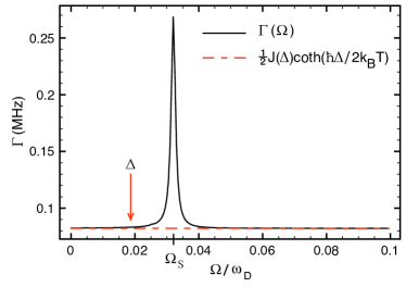
Figure 2: Rate $\Gamma$, Eq. 14, as a function of the driven field frequency $\Omega$ (solid line). There is a very pronounced peak at the region close to $\Omega_{s}$. Dashed line represents the rate $\Gamma$ for the non-driven case, $\epsilon_{0}=0$. Temperature used $T\approx 1K$.

$$\gamma\approx\tilde{r}_{5}=\sum_{i=0}^{2}\frac{C_{i}}{2\pi}\int_{0}^{\omega_{D}}d\omega\coth\left(\frac{\hbar\omega}{2k_{B}T}\right)J\left(\omega\right)\text{P}\left[\frac{1}{\omega-\Omega^{(i)}}-\frac{1}{\omega+\Omega^{(i)}}\right].$$ (13)

This expression is very similar to that found in the non-perturbative treatment of the atom-field interaction mandel . However, it is worth noting that Eq. (13) is derived here as a temperature dependent function.

The rates appearing in Eq. (11) and (12) can be written approximately as $\Gamma_{R}\approx\left(1-\frac{2f^{2}(\epsilon_{0},\Omega)}{1+2f^{2}(\epsilon_{0},\Omega)}\frac{\Delta(\Delta-2\gamma)}{\Omega^{2}}\right)\Gamma,$ and $\Gamma_{0}=2\Gamma_{1}=2\Gamma_{2}=2\Gamma$, where

$$\Gamma\approx\tilde{r}_{3}=\frac{1}{2}\sum_{i=0}^{2}C_{i}J(\Omega^{(i)})\coth\left(\frac{\hbar\Omega^{(i)}}{2k_{B}T}\right).$$ (14)

Figure 2 presents the rate $\Gamma$ as a function of the driven field frequency $\Omega$. It is clear that there is a signature of the peak of spectral density $J_{eff}\left(\omega\right)$ in its behavior. Close to the peak, $\Omega\approx\Omega_{s}$, the rate $\Gamma$ can be several orders of magnitude higher than the asymptotic value $\frac{1}{2}J\left(\Delta\right)\coth\left(\hbar\Delta/2k_{B}T\right)$. This result shows which regime of frequency must be avoided to obtain the largest relaxation time of the system.

Finally, the coefficients can be written as

$$\sigma_{x}\left(\infty\right) \approx \left(\frac{1}{1+2f^{2}(\epsilon_{0},\Omega)}\right)\tanh\left(\frac{\hbar\Delta}{2k_{B}T}\right),$$

$$G \approx \frac{\epsilon_{0}}{\Omega}f\left(\epsilon_{0},\Omega\right)\sigma_{x}\left(\infty\right),$$

$$H_{0} \approx -2H_{2}\approx-2G,\leavevmode\nobreak\ H_{1}\approx\left(\frac{\epsilon_{0}}{\omega_{1}}\right)^{2}\sigma_{x}\left(0\right).$$

The function

$$f\left(\epsilon_{0},\Omega\right)=\epsilon_{0}\frac{\Omega}{\Omega^{2}-\Delta\left(\Delta-2\gamma\right)},$$

gives a measure of the effects of the driven field on the spin dynamics. As expected, there are two important features to be considered: one is its intensity $\hbar\epsilon_{0}/g\mu_{B}$; and the other is how distant $\Omega$ is from the shifted natural resonance frequency $\sqrt{\Delta\left(\Delta-2\gamma\right)}\approx\Delta-\gamma$.

In the limit $\epsilon_{0}\rightarrow 0$, we obtain $\sigma_{x}\left(t\right)\approx\sigma_{x}\left(\infty\right)+\left(\sigma_{x}\left(0\right)-\sigma_{x}\left(\infty\right)\right)e^{-\Gamma t}$, where $\Gamma$ is the well-known expressionleggett $\Gamma=\frac{1}{2}J(\Delta)\coth(\hbar\Delta/2k_{B}T)$, and $\sigma_{x}(\infty)=\tanh\left(\frac{\hbar\Delta}{2k_{B}T}\right)$ is exactly the expected thermodynamical mean value. For the resonant case $\Omega\approx\Delta-\gamma$, we have $f(\epsilon_{0},\Delta-\gamma)\rightarrow\infty$, which implies $\sigma_{x}\left(t\right)\approx\sigma_{x}(0)e^{-\Gamma t}\cos(\epsilon_{0}t)$. The system evolves with a frequency imposed by the external driving field, and relaxes to a state where both spin components are equally probable. A detailed description of those phenomena is presented in the next section.

IV Discussion and conclusions

Figures 3-6 present the expectation values of $\hat{\sigma}_{x}$ and $\hat{\sigma}_{z}$ for the near resonance, $\Omega\approx\Delta-\gamma$, and the off-resonance, $\Omega=\Delta$, cases. Here we assume $\hbar\Delta\gg k_{B}T$, $\Delta\approx\Omega_{s}/2$, $\epsilon_{0}/\Delta\approx 0.03$ and $\omega_{D}/\ell\approx 750$.

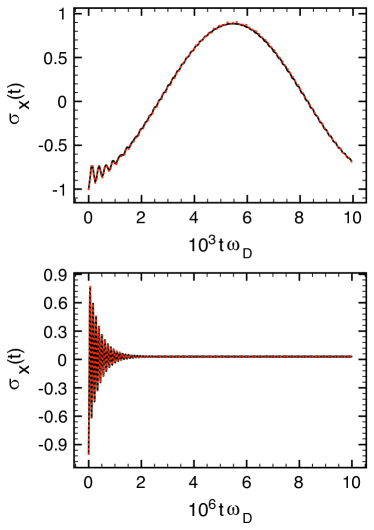
Figure 3: Time evolution of the expectation value of $\hat{\sigma}_{x}$ for the near resonance case $\Omega\approx\Delta-\gamma$. First plot presents the initial dynamics, where two well defined oscillation frequencies can be seen. For times $t<1/\ell$, damped oscillations due the poles of $J_{eff}(\omega)$, with relaxation time $1/\ell$, are observed. In the long time regime, $t>1/\ell$, the system evolves with oscillation frequency $\epsilon_{0}$ and, initially, with large amplitudes (reflecting the tuning between the frequency of the driving field and the natural frequency of the system). Due to the dissipative process, the system tends, in the time scale $1/\Gamma$, to an equal probability state for spin up and down, vanishing the average of $\hat{\sigma}_{x}$ (second plot). For very long times, $t\gg 1/\Gamma$, the system reaches a stationary state, oscillating with frequency $2\Omega$ and very small amplitude. Here we assumed $\omega_{D}/\ell=750$. Solid and dashed curves represent the numeric and the analytic results obtained.

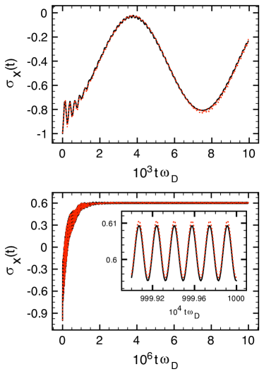
Figure 4: Time evolution of the expectation value of $\hat{\sigma}_{x}$ for the off-resonance $\Omega=\Delta$ case . Likewise the resonant case, the initial dynamics is composed of two well defined oscillation frequencies (first plot). Again, the contributions due the poles of $J_{eff}(\omega)$ vanish after times $t\approx 1/\ell$. In the long time regime, $t>1/\ell$, the system evolves oscillating with frequency $\approx\sqrt{\epsilon_{0}^{2}+\gamma^{2}}$, and the amplitude observed is not as larger as in the resonant case. The second plot presents the dynamics for the long time regime. As one can see, the system tends to approach the stationary state at the same time scale as the resonance case, however we see that $\sigma_{x}(t\rightarrow\infty)$ is now much closer to its thermodynamical equilibrium value for $\epsilon_{0}=0$, $\tanh(\hbar\Delta/2k_{B}T)\approx 1$. Once again, for very long times, $t\gg 1/\Gamma$, (inset second plot) the system oscillates with frequency $2\Omega$ and very small amplitude. Here we assumed $\omega_{D}/\ell=750$. Solid and dashed curves represent the numeric and the analytic results obtained.

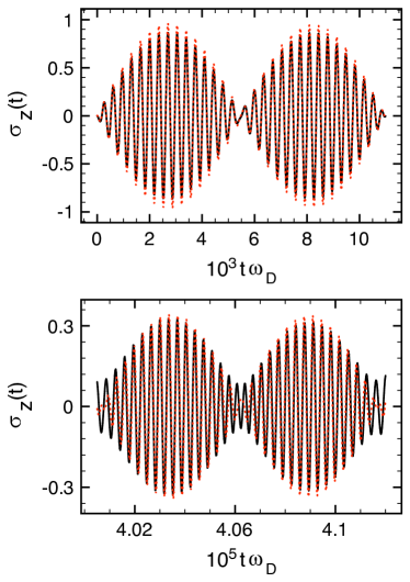
Figure 5: Time evolution of the expectation value of $\hat{\sigma}_{z}$ for the near resonance case $\Omega\approx\Delta-\gamma$. The initial $\sigma_{z}$ dynamics behavior (first plot) is characterized by a clear structure of beats, with beat and angular frequency given by $\omega_{1}$ and $\Omega+\omega_{1}/2$. Due the decoherence processes, the modes related with the frequencies $\omega_{i}$ evanesce in the characteristic time $1/\Gamma$, destroying the beat structure (second plot), for which arises an oscillatory regime of same frequency $\Omega$ of the applied field. Here we assumed $\omega_{D}/\ell=750$. Solid and dashed curves represent the numeric and the analytic results obtained.

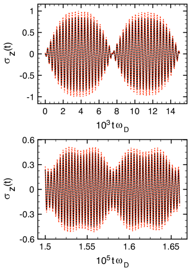
Figure 6: Time evolution of the expectation value of $\hat{\sigma}_{z}$ for the off-resonance case $\Omega\approx\Delta$. The same behavior for the resonant case is observed. The initial $\sigma_{z}$ dynamics behavior (first plot) is characterized by a clear structure of beats, with beat and angular frequencies given by $\omega_{1}$ and $\Omega+\omega_{1}/2$. Due the decoherence processes, the modes related with the frequencies $\omega_{i}$ evanesce in the characteristic time $1/\Gamma$, destroying the beat structure (second plot), for which an oscillatory regime of same frequency $\Omega$ of the applied field arises. Here we assumed $\omega_{D}/\ell=750$. Solid and dashed curves represent the numeric and the analytic results obtained.

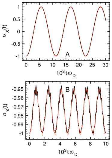
Figure 7: The time evolution of the expectation value $\sigma_{x}\left(t\right)$ using the approximate analytic solution Eq.11 (dashed line) and the exact numeric calculation (solid line). Plot A presents the behavior for the resonance case $\Omega\approx\Delta-\gamma$. The oscillation frequency observed is $\omega_{1}\approx\epsilon_{0}$. Plot B shows the case off resonance, $\Omega=0.8\Delta$. The main oscillation frequency is $\omega_{1}$. The estimate relaxation time for these plots is $T_{1}=12\mu s$. The temperature used is $T\approx 1K$.

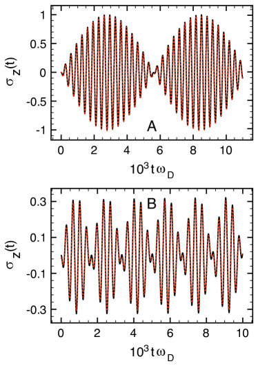
Figure 8: The time evolution of the expectation value $\sigma_{z}\left(t\right)$ using the approximate analytic solution Eq.11 (dashed line) and the exact numeric calculation (solid line). Plot A presents the behavior for the resonance case $\Omega\approx\Delta-\gamma$. $\omega_{1}$ and $\Omega-\omega_{1}/2$ are the beat and the angular frequencies respectively. Plot B shows the case off resonance $\Omega=0.8\Delta$. We can identify approximately the beat and angular frequencies as $\omega_{1}$ and $\Omega+\omega_{1}/2$. The temperature used is $T\approx 1K$.

It is well known sakurai that, in the absence of dissipation, the system would indefinitely evolve into coherent cycles of absorption and emission of energy - the Rabi oscillations. Furthermore, the change in the spin up and down populations exhibits an oscillatory time dependence with frequency $\sqrt{\epsilon_{0}^{2}+(\Omega-\Delta)^{2}}$, and amplitude $\epsilon_{0}^{2}/(\epsilon_{0}^{2}+(\Omega-\Delta)^{2})$. It is worth noting that under the resonance condition, $\Omega=\Delta$, the oscillating field fully drives the transitions between up and down spin states and that the weaker the driving field, the narrower the resonance peak. As one can notice by inspecting figures 3 and 4, the coupling system-bath changes some of those features. First of all, the resonance condition is no longer verified at the frequency associated with the static applied field. Now, the new natural frequency is given by $\Omega=\Delta-\gamma$, where the shift $\gamma$, Eq. (13), is completely associated with the coupling between the system and its reservoir - Lamb shift. This is exactly the behavior we have for the first plots of figures 3 and 4: the largest amplitudes of oscillation occur for those frequencies closest to the new resonance condition. As expected, the component $\sigma_{x}$ oscillates with frequency $\epsilon_{0}$ at resonance, and $\sqrt{\epsilon_{0}^{2}+\gamma^{2}}$ for the off-resonance $\Omega=\Delta$ case. Another important change in the spin dynamics is that the system does not evolve indefinitely in coherent cycles of absorption and emission of energy. In fact, the dissipation process induced by the coupling to the dissipative bath destroys the coherence in the emission-absorption cycles and, after a long time, decoherence takes place. Indeed, the behavior of the expectation value of $\sigma_{x}(t)$ in the long time regime (figures 3 and 4), reveals this decoherence process. As one can see, the large amplitude of oscillations observed initially, a consequence of the coherent emission-absorption stimulated by the field, tends to decrease in time. This process occurs in a time scale given by $1/\Gamma$, Eq. (14), which has almost the same value as presented in figures 3 and 4. This happens because for both cases we are away from the peak of the rate $\Gamma$, Figure 2, where it is practically a constant given by $\frac{1}{2}J(\Delta)\coth(\hbar\Delta/2k_{B}T)$. For very long times, $t\gg 1/\Gamma$, the system reaches a stationary state, oscillating with frequency $2\Omega$ (inset of figure 4) and small amplitude around the asymptotic value $\sigma_{x}(t\rightarrow\infty)$. Here we observe that this asymptotic value changes dramatically when we leave the resonance condition. This feature can be understood as follows. At resonance, the driving field causes perfect transitions between up and down eigenstates of $\hat{\sigma}_{x}$, but because the system-bath coupling destroys the coherence along the process, we see that after a very long time, $t\gg 1/\Gamma$, a completely random emission-absorption process sets in and makes the expectation value of $\hat{\sigma}_{x}$ vanish. For the off-resonance case, the driving field no longer produces 100$\%$ probability transitions in the system. Again, the coupling with the bath destroys the coherence of this process, and favours the occupation of the lowest energy state. Thus, as we are considering a small applied field, i.e, $\epsilon_{0}/\Delta\ll 1$, the bath drives the system towards its thermodynamical equilibrium state at zero driving field, $\sigma_{x}\rightarrow\tanh\left(\frac{\hbar\Delta}{2k_{B}T}\right)$. Since we have assumed $\hbar\Delta\gg k_{B}T$, this implies $\tanh\left(\frac{\hbar\Delta}{2k_{B}T}\right)\approx 1$. How close the system will approach that asymptotic value depends on both the intensity and frequency of the driving field.

All the features discussed so far were general consequences of the system-bath interaction, and do not depend on the specific form of the spectral density of the bath. Nevertheless, the first plots of figures 3 and 4 show a particular behavior for short times: two well defined regimes of oscillation frequencies can be observed. This phenomenon is a signature of the rich structure of the effective spectral density, Eq. (3). In fact, because $J_{eff}(\omega)$ has poles in the complex plane, new modes of oscillation arise in the spin dynamics. Those new modes have lifetimes imposed by the imaginary part of the poles, whereas the natural frequencies of the system are shifted by their real part. As we could observe from $J_{eff}(\omega)$ (3), the most important modes ( those with long lifetimes and measurable amplitude of oscillations) due to the poles are associated with the peak of $J_{eff}(\omega)$, at which a strong correlation between orbital and spin degrees of freedom takes place. These modes, (see the first term of Eq. (11)), have lifetimes determined by the width $\ell$ of the bath resonance, and frequencies $\Omega_{s}-\Omega^{(i)}$, with $\Omega^{(0)}=\Omega$, $\Omega^{(1)}=\Omega-\epsilon_{1}$ and $\Omega^{(2)}=\Omega+\epsilon_{1}$. The amplitude of oscillation, assuming a weak driving field, $\epsilon_{0}/\Delta\ll 1$, can be approximated by $\frac{2\ell J(\Omega_{s})}{(\Omega_{s}-\Delta)^{2}}$ (for $\Delta\neq\Omega_{s}$). Therefore, if one experimentally reaches the conditions $\frac{2\ell J(\Omega_{s})}{(\Omega_{s}-\Delta)^{2}}\approx O(1)$ and $\ell/\Delta\ll 1$, it would be possible to determine some physical parameters of spin-bath coupling, e.g., the electron-phonon constant coupling $\delta_{s}$.

Figures 5 and 6 show the $\sigma_{z}$ component for the same conditions previously discussed. As it can be noticed, there is a clear structure of beats in its dynamical behavior. At resonance, figure 5, the beat and angular frequencies are, respectively, given by $\omega_{1}$ and $\Omega+\omega_{1}/2$. For this component we do not verify two oscillatory regimes for times of the order of $1/\ell$. This occurs because of the suppression of the pole’s contribution by the strong oscillations of the remaining terms. As a consequence of the decoherence process imposed by the bath of oscillators, other important feature is that, for long times, the modes related with the frequencies $\omega_{i}$ evanesce, destroying the beat structure. These modes are associated with the coherent oscillations due to the driving field. Thus, after a long time, only an oscillatory regime of frequency $\Omega$ remains. The characteristic time for that is of the order of $1/\Gamma$. The regime slightly off resonance $\Omega=\Delta$, figure 6, practically does not change. In this case the beat and angular frequencies are given respectively by $\omega_{1}$ e $\Omega-\omega_{1}/2$. This shows that the component $\sigma_{z}$ is not so sensitive to how close the external field frequency is to the natural resonance frequency of the spin. As it is directly coupled to the external field, this component has a stronger dependence on its amplitude.

Now, we will focus on the specific case in which we use bulk physical parameters for typical quantum dots size. We assume here the piezoelectric electron-phonon interaction , $s=3$, and quantum dots frequencies $\omega_{0}\equiv 15$meV. The external fields applied to the dots are assumed to be such that $\hbar\Delta/k_{B}=6.7K$ and $\hbar\epsilon_{0}/k_{B}=0.2K$, and the Debye frequency $\hbar\omega_{D}/k_{B}=360K$. Figures 7 and 8 present the $\sigma_{x}$ and $\sigma_{z}$ dynamics using the bulk physical parameters $\beta=3000m/s$, $m^{\ast}=0.063m_{e}$ and $\delta_{3}=355$. The temperature used for the calculation is $T\approx 1K$.

The plots A in figures 7 and 8 show the dynamics of the expectation values $\sigma_{x}\left(t\right)$ and $\sigma_{z}\left(t\right)$, respectively, for the case close to the resonance, $\Omega\approx\Delta-\gamma$. We can see that the dynamics of $\sigma_{x}$ has a well defined frequency of oscillation, given by $\omega_{1}\approx\epsilon_{0}$, with amplitude close to $|\sigma_{x}(0)|$. Because of the weak coupling limit, the terms in Eq. (11) due to the poles of the spectral density are negligible compared to the others. Therefore, this explains why we do not distinguish between several different regimes of relaxation. The relaxation time $T_{1}$ is estimated to be of the order of $1/\Gamma=12\mu s$. For the $\sigma_{z}$ component we see the expected beat structure, with well characterized beat and angular frequencies given by $\omega_{1}$ and $\Omega-\omega_{1}/2$, respectively.

The plots B in figures 7 and 8 present the dynamics for a case off resonance, $\Omega=0.8\Delta$. Now we can see that several frequencies contribute to the spin dynamics. For $\sigma_{x}$, the main oscillation frequency is still $\omega_{1}$, however the amplitude of oscillations has decreased more than one order of magnitude. The $\sigma_{z}$ dynamics has also changed. There is still a structure of beats but more frequencies appear in the spectral decomposition. $\omega_{1}$ and $\Omega+\omega_{1}/2$ are the beat and angular frequencies for this case. For the very long time regime, $t\gg 1/\Gamma$, the component $\sigma_{x}$ reaches the stationary equilibrium oscillating with frequency $2\Omega$ and very small amplitude $G$, around the value $\sigma_{x}(\infty)$. For $\sigma_{z}$ we observe that the beat structure disappears, giving place to oscillations of frequency $\Omega$ and constant amplitude $\frac{2\Delta}{\Omega}f(\epsilon_{0},\Omega)(\sigma_{x}(\infty)+G/2)$.

In conclusion we have obtained approximate analytic solutions for the Blcoh-Redfield equations of dissipative spins in a driving field. The complex structure presented by the effective bath spectral density brings a richer dynamical behavior for the spin trapped in a quantum dot. We showed that the existence of the peak in the spectral density introduces a new temporal scale in the problem, $1/\ell$, the peak’s width, which clearly separates distinct time evolutions of the component $\sigma_{x}$. The first one, short times, $t\ll 1/\ell$, is basically determined by the characteristics of the peak. We saw that the oscillations presented in this regime have their natural frequencies shifted by the bath resonance, $\Omega_{s}$, and their lifetimes are determined by $1/\ell$. Thus, in principle, this regime could be used to infer intrinsic quantities of the system-bath coupling , such as the electron-phonon constant $\delta_{s}$. On the other hand, the long time regime, $t\gg 1/\ell$, was shown to be governed by the external fields. We found that the relaxation rate $\Gamma$ for this regime presents a strong peak for frequencies close to the bath resonance, revealing the signature of the effective spectral density. In addition, we were able to identify the shift induced by the system-bath coupling in the natural frequencies of the system. We found that this shift, $\gamma$, has the form of a temperature dependent Lamb shift mandel

V Acknowledgments

FB was supported by Fundação de Amparo à Pesquisa do Estado de São Paulo (FAPESP), contract 01/05748-6. HW and AOC acknowledge support from the Conselho Nacional de Desenvolvimento Científico e Tecnológico(CNPq) and Hewlett-Packard Brasil. AOC also thanks The Millenium Institute for Quantum Information. We would like to thank David DiVincenzo for a critical reading of the manuscript.

VI Appendix

In this section we present the explicit form for the Bloch-Redfield coefficients used in the main text.

The first step is to construct the matrix elements of the non-dissipative time evolution operator $U(t,t^{\prime})$,

$$\text{Im}U_{RR}(t,t^{\prime})U_{RL}(t,t^{\prime}) = \frac{\cos^{2}(\phi)}{4}\bigg{(}\sin[(t-t^{\prime})\Omega]+\sin[(t+t^{\prime})\Omega](1-\cos[(t-t^{\prime})\epsilon_{1}])\bigg{)}$$

$$+\frac{(1+\sin(\phi))^{2}}{8}\sin[(t-t^{\prime})(\Omega+\epsilon_{1})]+\frac{(1-\sin(\phi))^{2}}{8}\sin[(t-t^{\prime})(\Omega-\epsilon_{1})],$$

$$\text{Re}U_{RR}(t,t^{\prime})U_{RL}(t,t^{\prime}) = \frac{\cos(\phi)}{2}\sin(t^{\prime}\Omega)\sin[(t-t^{\prime})\epsilon_{1}]-\frac{\sin(2\phi)}{4}\cos(t^{\prime}\Omega)(1-\cos[(t-t^{\prime})\epsilon_{1}]),$$ (15)

$$|U_{RR}(t,t^{\prime})|^{2}-|U_{RL}(t,t^{\prime})|^{2} = \frac{\cos^{2}(\phi)}{2}\bigg{(}\cos[(t-t^{\prime})\Omega]+\cos[(t+t^{\prime})\Omega](1-\cos[(t-t^{\prime})\epsilon_{1}])\bigg{)}$$

$$+\frac{(1+\sin(\phi))^{2}}{4}\cos[(t-t^{\prime})(\Omega+\epsilon_{1})]-\frac{(1-\sin(\phi))^{2}}{4}\cos[(t-t^{\prime})(\Omega-\epsilon_{1})].$$

If the limit $\frac{J(\omega)}{\omega}|_{\omega\rightarrow 0}$ exists, and $J(\omega)$ does not have poles in the real axis, we can write the real and imaginary parts of $M(t)$ as ${\rm{Re}}[M(t)]=\frac{1}{\pi}\int_{0}^{\infty}d\omega J(\omega)\cos(\omega t)\coth(\beta\hbar\omega/2)$ and ${\rm{Im}}[M(t)]=-\frac{1}{\pi}\int_{0}^{\infty}d\omega J(\omega)\sin(\omega t)$, respectively. Now we are in position to calculate the coefficients $A_{i}(t)$ and $\Gamma_{ij}(t)$. As pointed out previously, if we first perform the time integrals, we can reach very useful expressions for the frequency analysis of our problem. Following this procedure, we obtain the fluctuation coefficients $A_{x}$ and $A_{y}$ and the rate $\Gamma_{xx}(t)$ as (with analogous expressions for $\Gamma_{xz}(t),$ and $\Gamma_{yz}(t)$)

$$A_{x}(t) = -\frac{\cos^{2}(\phi)}{2\pi}\bigg{(}1-\cos(2\Omega t)\bigg{)}I_{1}^{(0)}[\Omega;J(x),t]-\left(\frac{\cos^{2}(\phi)\cos(2\Omega t)+(1+\sin(\phi))^{2}}{4\pi}\right)I_{1}^{(0)}[\Omega+\epsilon_{1};J(x),t]$$ (16)

$$-\left(\frac{\cos^{2}(\phi)\cos(2\Omega t)+(1-\sin(\phi))^{2}}{4\pi}\right)I_{1}^{(0)}[\Omega-\epsilon_{1};J(x),t]-\frac{\cos^{2}(\phi)}{2\pi}\sin(2\Omega t)\bigg{(}I_{2}^{(0)}[\Omega;J(x),t]$$

$$-\frac{1}{2}(I_{2}^{(0)}[\Omega+\epsilon_{1};J(x),t]+I_{2}^{(0)}[\Omega-\epsilon_{1};J(x),t])\bigg{)},$$

$$A_{y}(t) = \frac{\sin(2\phi)}{2\pi}\bigg{(}\sin(\Omega t)I_{1}^{(0)}[\Omega;J(x),t]+\cos(\Omega t)I_{2}^{(0)}[\Omega;J(x),t]\bigg{)}$$ (17)

$$-\frac{\cos(\phi)}{2\pi}\sin(\Omega t)\bigg{(}(1+\sin(\phi))I_{1}^{(0)}[\Omega+\epsilon_{1};J(x),t]-(1-\sin(\phi))I_{1}^{(0)}[\Omega-\epsilon_{1};J(x),t]\bigg{)}$$

$$-\frac{\cos(\phi)}{2\pi}\cos(\Omega t)\bigg{(}(1+\sin(\phi))I_{2}^{(0)}[\Omega+\epsilon_{1};J(x),t]-(1-\sin(\phi))I_{2}^{(0)}[\Omega-\epsilon_{1};J(x),t]\bigg{)},$$

$$\Gamma_{xx}(t) = \frac{\cos^{2}(\phi)}{2\pi}\left[\bigg{(}1+\cos(2\Omega t)\bigg{)}I_{3}[\Omega,T,t]-\sin(2\Omega t)\bigg{(}I_{4}[\Omega,T,t]-\frac{1}{2}(I_{4}[\Omega+\epsilon_{1},T,t]+I_{4}[\Omega-\epsilon_{1},T,t])\bigg{)}\right]$$

$$-\left(\frac{\cos^{2}(\phi)\cos(2\Omega t)-(1+\sin(\phi))^{2}}{4\pi}\right)I_{3}[\Omega+\epsilon_{1},T,t]-\left(\frac{\cos^{2}(\phi)\cos(2\Omega t)-(1-\sin(\phi))^{2}}{4\pi}\right)I_{3}[\Omega-\epsilon_{1},T,t],$$

where we have defined the integrals

$$I_{1}[y,t] \equiv \frac{1}{2}\int_{0}^{\infty}d\omega J(\omega)\left(\frac{\sin((\omega-y)t)}{\omega-y}-\frac{\sin((\omega+y)t)}{\omega+y}\right),$$

$$I_{2}[y,t] \equiv \int_{0}^{\infty}d\omega J(\omega)\left(\frac{\sin^{2}((\omega-y)\frac{t}{2})}{\omega-y}+\frac{\sin^{2}((\omega+y)\frac{t}{2})}{\omega+y}\right).$$ (19)

$$I_{3}[y,T,t] \equiv \frac{1}{2}\int_{0}^{\infty}d\omega J(\omega)\coth\left(\frac{\hbar\omega}{2k_{B}T}\right)\left(\frac{\sin((\omega-y)t)}{\omega-y}-\frac{\sin((\omega+y)t)}{\omega+y}\right),$$

$$I_{4}[y,T,t] \equiv \int_{0}^{\infty}d\omega J(\omega)\coth\left(\frac{\hbar\omega}{2k_{B}T}\right)\left(\frac{\sin^{2}((\omega-y)\frac{t}{2})}{\omega-y}+\frac{\sin^{2}((\omega+y)\frac{t}{2})}{\omega+y}\right).$$ (20)

The special form of the integrals $I_{n}$ allows us to find approximate analytic expressions, which are asymptotically exact for $t\rightarrow\infty$. Considering that $J\left(\omega\right)$ satisfies the conditions $J\left(0\right)=J\left(\infty\right)\rightarrow 0$, we can write for $t\gg 1/\Omega_{c}$,

$$I_{1}\left(y,t\right)\approx\frac{\pi}{2}J\left(y\right)+\frac{\pi}{2}\left\{\text{Res}\left[J\left(z_{0}\right)\frac{e^{it(z_{0}-y)}}{z_{0}-y}\right]+\text{Res}\left[J\left(z_{0}\right)\frac{e^{-it(z_{0}-y)}}{z_{0}-y}\right]\right\}$$

$$-\frac{\pi}{2}\left\{\text{Res}\left[J\left(z_{0}\right)\frac{e^{it(z_{0}+y)}}{z_{0}+y}\right]+\text{Res}\left[J\left(z_{0}\right)\frac{e^{-it(z_{0}+y)}}{z_{0}+y}\right]\right\},$$ (21)

$$I_{2}\left(y,t\right)\approx\frac{1}{2}\int_{0}^{\Omega_{c}}d\omega J\left(\omega\right)\text{P}\left[\frac{1}{\omega-y}+\frac{1}{\omega+y}\right]-\frac{i\pi}{2}\left\{\text{Res}\left[J\left(z_{0}\right)\frac{e^{2it(z_{0}-y)}}{z_{0}-y}\right]-\text{Res}\left[J\left(z_{0}\right)\frac{e^{-2it(z_{0}-y)}}{z_{0}-y}\right]\right\}$$

$$-\frac{i\pi}{2}\left\{\text{Res}\left[J\left(z_{0}\right)\frac{e^{2it(z_{0}+y)}}{z_{0}+y}\right]-\text{Res}\left[J\left(z_{0}\right)\frac{e^{-2it(z_{0}+y)}}{z_{0}+y}\right]\right\},$$ (22)

and similar expressions for $I_{3}$ and $I_{4}$. The residues in the above expressions are calculated for the poles of $J\left(\omega\right)$ inside of the semi-circle centered at $z=\Omega_{c}$ and radius $\Omega_{c}$. In this calculation, we have assumed that $y$ is not a pole of the function $J\left(\omega\right)$. Here we have replaced the upper limit of integration by the cutoff frequency $\Omega_{c}$.

Expressions (21) and (22) show us that the time-dependent terms of $I_{n}$ have lifetimes determined by the imaginary part of the poles of $J\left(\omega\right)$ in the complex plane. In our case, the poles of $J\left(\omega\right)$ correspond to those of $J_{eff}\left(\omega\right)$ defined by Eq.3.

Figure 9 sketches the $I_{1}$ and $I_{2}$ behaviors assuming $J(\omega)$ as an Ohmic function $J(\omega)=0.05\omega e^{-20\omega}$ and the spectral density $J_{eff}(\omega)$ (Eq. 3). Comparing the results using the analytic form Eqs. 21-22 and the exact numeric calculation, we find a good agreement for $t\gg 1/\omega_{D}$, specially for the case $g(\omega)=J_{eff}(\omega)$ where the terms due the poles dominate the short time regime, $t\leq 1/\ell$.

Figure 9: $I_{1}^{(0)}[y;g(\omega),t]$ and $I_{2}^{(0)}[y;g(\omega),t]$ integrals evaluated using the analytic solutions Eqs.(21-22) (dashed lines) and the exact numeric calculations (solid lines). Plots A and B present the integrals computed for an Ohmic function $g(\omega)=0.05\omega e^{-20\omega}$. Plots C and D assume $g(\omega)$ as the spectral density $J_{eff}(\omega)$ (Eq. 3).

References

- (1) M. A. Nielsen and I. L. Chuang, Quatum computation and quantum information, (Cambridge Univ. Press, Cambridge, 2000).
- (2) Guido Burkard: Theory of solid state quantum information processing, cond-mat/0409626, 23 Sep 2004.
- (3) A. J. Leggett et al.: Dynamics of the dissipative two-state system, Rev. Mod. Phys. 59, 1 (1987).
- (4) A. O. Caldeira and A. J. Leggett: Influence of damping on quantum interference: an exactly soluble model, Phys. Rev. A 31, 1059 (1985).
- (5) Guido Burkard, Daniel Loss and David P. DiVincenzo: Coupled quantum dots as quantum gates, Phys. Rev. B 59, 2070 (1999).
- (6) Daniel Loss and David P. DiVincenzo: Quantum computation with quantum dots, Phys. Rev. A 57, 120 (1998).
- (7) F. H. L. Koppens et al.: Driven coherent oscillations of a single electron spin in a quantum dot, Nature 442, 766 (2006).
- (8) Alexander V. Khaetskii and Yuli V. Nazarov: Spin relaxation in semiconductos quantum dots, Phys. Rev. B 61, 12639 (2001)
- (9) E. L. Ivchenko and G. E. Pikus, Superlattices and other heterostructures (2nd Edition, Springer, Berlin, 1997)
- (10) Sigurdur I. Erlingsson and Yuli V. Nazarov: Hyperfine-mediated transitions between a Zeeman split doublet in GaAs quantum dots: The role of the internal field, Phys. Rev. B 66, 155327 (2002).
- (11) Miro Kroutvar et al.: Optically programmable electron spin memory using semiconductor quantum dots, Nature 432, 81 (2004).
- (12) J. M. Elzerman et al.: Single-shot read-out of an individual electron spin in a quantum dot , Nature 430, 431 (2004).
- (13) Harry Westfahl Jr. et al.: Dissipative dynamics of spins in quantum dots, Phys. Rev. B 70, 195320 (2004).
- (14) Alexander V. Khaetskii and Yuli V. Nazarov: Spin-flip transitions between Zeeman sublevels in semiconductors quantum dots, Phys. Rev. B 64, 125316 (2001).
- (15) P. Y. Yu and M. Cardona, Fundamentals of Semiconductors, (Springer-Verlag, New York, 2001).
- (16) Ludwig Hartmann et al.: Driven Tunneling Dynamics: Bloch-Redfield Theory versus Path Integral Approach, Phys. Rev. E 61, R4687 (2000).
- (17) L. Mandel and E. Wolf, Optical Coherence and Quantum Optics (Cambridge, New york, 1995).
- (18) J. J. Sakurai, Modern Quantum Mechanics, Addison Wesley, (MA, US 1995).
- (19) L. Jacak, P. Hawrylak and A. Wjs, Quantum dots, (Springer, Berlin, 1998).
- (20) V. N. Golovach, Alexander Khaetskii and Daniel Loss: Phonon-Induced decay of the electron spin in quantum dots, Phys. Rev. Lett. 93, 016601 (2004).
- (21) P. Dennery and A. Krzywicki, Mathematics for physicists, Dover (Mineola, NY 1996).