Dynamical diversity and metastability in a hindered granular column near jamming

Abstract

Granular media jam into a panoply of metastable states. The way in which these states are achieved depends on the nature of local and global constraints on grains; here we investigate this issue by means of a non-equilibrium stochastic model of a hindered granular column near its jamming limit. Grains feel the constraints of grains above and below them differently, depending on their position. A rich phase diagram with four dynamical phases (ballistic, activated, logarithmic and glassy) is revealed. The statistics of the jamming time and of the metastable states reached as attractors of the zero-temperature dynamics is investigated in each of these phases. Of particular interest is the glassy phase, where intermittency and a strong deviation from Edwards’ flatness are manifest.

1 Introduction

Granular media are by now recognised as being paradigms of complexity comp , especially near their jamming limit sidjamming . The fact that most grains are too large to be perturbed by the effect of room temperature leads to an ‘athermal’ dynamics, which is a major cause of this complexity – configurations once generated, are remembered, and their hysteretic effects persist in any ensuing dynamics, and the new configurations generated therefrom. Another origin of complexity in such systems is their generic disorder; this leads in particular to a random landscape of metastable states being explored if a granular system is suitably ‘quenched’, rather than a crystallisation into an appropriate ordered state. The way in which this landscape is explored depends strongly on the driving forces applied, in the absence of any real thermodynamics.

The work we present here is an attempt to explore many of these issues, in particular those to do with the nature of ground states in a system near jamming, and how these are reached. This is the main motivation for our focusing on the effect of ‘zero-temperature’ dynamics on the model we will later introduce, since zero-temperature dynamics are known to be the route to systemic ground states. Another aspect of interest around which our model was designed was the exploration of spatial inhomogeneities, to answer questions such as: how does position along a column of grains influence the dynamics observed there? This is an important question for several reasons, one of the earliest being that experimental measurements of density along a column of grains revealed wide variations sid , depending on whether they were near the top, the bottom or the middle – in its turn, this implied that the compactivity of the system edwards was non-uniform. A more visible manifestation of spatial inhomogeneities is the presence of force chains bob and bridge networks bridges , which are unique signatures of the granular state.

Given the complexity of issues we wish to investigate, we have chosen a minimal model to work with, whose ingredients are based on our experience with several earlier ones I ; II ; III ; IV . A feature that all the models share is that of orientational disorder; every grain is allowed to occupy one of two states, corresponding to ‘ordered’ and ‘disordered’. Disordered orientations generate voids and waste space, whereas ordered ones do not. Implicit in this description is the effect of shape, which is most easily understood in terms of the rectangular grains of aspect ratio $a$ considered in I ; II . Grains aligned along their long edges (length $1$) result in a fully packed column, whereas those perched on their short edges (length $a$) leave voids of size $1-a$. The horizontal orientation is thus ordered, and the vertical one disordered.

Our models became progressively more sophisticated. The earliest model of rectangular grains considered in I ; II was strictly non-interacting, with the only effects included being due to gravity and excluded volume – grains could not overlap, and those that were deeper in a column were less free to move. One of the major extensions in III ; IV was the introduction of the shape parameter $\varepsilon$ to include grains of arbitrary, i.e., non-rectangular shape – such grains can have multiply many orientations in reality, but the two-state description was retained in the interests of simplicity. The parameter $\varepsilon$ was allowed to vary over all rational and irrational numbers, with a view to describing regular and irregular grains, as will be explained further below.

Another difference between the two models was that the first one I ; II interpolated between jammed and fluidised regimes, whereas the second one was explicitly constructed to examine the jamming regime. In the latter case, it seemed reasonable to assume that translational diffusion was essentially absent, with all compaction occurring via orientational rearrangements – it was therefore appropriate to focus on a column, rather a box I ; II , of grains. Interactions were introduced in the column model of III ; IV such that every grain now not only felt the weight of grains above it, but was also constrained by all of their orientations. This modelling was appropriate as a representation of grains in the free surface layer, which were too far from the base to feel an undertow; in the jamming limit, however, such grains would be expected to feel the orientational constraints arising from grains above them.

The present model incorporates all of the above features, and generalises them to include the presence of orientational constraints arising from grains below a given grain. Unlike our previous models I ; II ; III ; IV , where interactions propagated downwards from the top, here they propagate both upwards and downwards. Clearly the extent of this propagation depends on grain position In this sense we model a column of grains with a top, a middle and a bottom.

We devote this paper to a comprehensive investigation of the ground states of this model, and how they are reached via zero-temperature dynamics. The main questions we will answer along the way will be related to several of the issues mentioned above; in particular the issue of spatial inhomogeneities will be relevant, since the dynamical regimes attainable via this model will depend on which part of the column – top, middle or bottom – is being examined. Additionally, we will see that there is a panoply of metastable ground states available to the system; the dynamics of their attainment will allow us to classify the appropriate regimes as ballistic, logarithmic, activated and glassy. The glassy regime is by far the most novel and interesting of these regimes, and will be investigated in greater depth than the others; its full exploration is, however, reserved for future work.

The plan of this paper is as follows. The definition of the model is given in Section 2. Section 3 contains an investigation of its static properties, with an emphasis on the ground states. Section 4 presents a study of zero-temperature dynamics: a rich phase diagram with four dynamical phases is revealed and investigated thoroughly. A discussion is presented in Section 5. Exact results for small systems, as well as other technical results, are presented in three appendices.

2 The model

Like the unhindered (fully directional) model described in III ; IV , the present model consists of a finite column of $N$ grains, labelled by their depth $n=1,\dots,N$. Each grain assumes two orientational states, which are referred to as ordered and disordered. We set $\sigma_{n}=+1$ (resp. $\sigma_{n}=-1$) if grain number $n$ is ordered (resp. disordered). A configuration of the column is therefore uniquely defined by the orientation variables $\{\sigma_{n}\}$. There are $2^{N}$ such configurations.

The model is defined by a stochastic dynamics which do not obey detailed balance. In the present context, detailed balance essentially means a symmetry in $m$ and $n$ on the dynamical effect of grain orientation $\sigma_{m}$ on $\sigma_{n}$. The expressions for the local fields (2.4), (2.7) clearly do not obey such ‘action and reaction’. Our model is therefore intrinsically out of equilibrium, and its stationary state at finite temperature is a genuine non-equilibrium steady state

More precisely, the model is defined as follows. Grains are selected in a random sequential fashion and updated with the orientation-flipping rates

$$\left\{\matrix{w(\sigma_{n}=+1\to\sigma_{n}=-1)=\exp\left(-\displaystyle{\displaystyle\lambda_{n}+H_{n}\over\displaystyle\Gamma}\right),\hfill\cr\cr w(\sigma_{n}=-1\to\sigma_{n}=+1)=\exp\left(-\displaystyle{\displaystyle\lambda_{n}-H_{n}\over\displaystyle\Gamma}\right),\hfill}\right.$$ (2.1)

where, along the lines of previous work I ; II ; III ; IV :

$\bullet$ $\Gamma$ is a dimensionless vibration intensity, referred to as temperature, and related to the ‘fast’ temperature in granular media.

$\bullet$ $\lambda_{n}$ is the activation energy felt by grain $n$. We make the assumption that it increases linearly with the depth $n$, but otherwise does not depend on grain orientations. We set

$$\lambda_{n}=\displaystyle{\displaystyle n\Gamma\over\displaystyle\xi_{\rm dyn}},$$ (2.2)

so that the local frequency

$$\omega_{n}=\exp\left(-\displaystyle{\displaystyle\lambda_{n}\over\displaystyle\Gamma}\right)=\exp\left(-\displaystyle{\displaystyle n\over\displaystyle\xi_{\rm dyn}}\right)$$ (2.3)

falls off exponentially, with a characteristic length $\xi_{\rm dyn}$. This dynamical length corresponds to the depth of the boundary layer beyond which grains are frozen out by the sheer weight of grains above them.

$\bullet$ $H_{n}$ is the local ordering field felt by grain $n$, which determines the orientational response of grain $n$ to the orientations $\{\sigma_{m}\}$ of all the other grains. In previous work III ; IV the local field $H_{n}$ only involved the uniform effect of the upper grains ($m=1,\dots,n-1$). In the present model, we also take into account the back-propagation from grains below a given grain $n$ ($m=n+1,\dots,N$). This effect cannot be similarly uniform. We assume for simplicity that upward interactions are exponentially damped, with a characteristic length $\xi_{\rm int}$, the interaction length. We therefore set

$$H_{n}=h_{n}+gj_{n},$$ (2.4)

where we denote by $h_{n}$ the uniform effect of grains above $n$ ($m=1,\dots,n-1$), and by $j_{n}$, the non-uniform effect of grains below $n$ ($m=n+1,\dots,N$), whose strength is measured by a small (positive) coupling constant $g$. Both components $h_{n}$ and $j_{n}$ of the local field contain the contribution of every single grain orientation $\sigma_{m}=\pm 1$ through the quantity $f(\sigma_{m})$. As before III ; IV , the latter assumes the following two values:

$$f(\sigma_{n})=\left\{\matrix{\varepsilon\hfill&\hbox{if}\hfill&\sigma_{n}=-1,\cr-1\ \hfill&\hbox{if}\hfill&\sigma_{n}=+1.}\right.$$ (2.5)

A useful equivalent formula is the following:

$$f(\sigma_{n})={\textstyle{\displaystyle{\displaystyle 1\over\displaystyle 2}}}(\varepsilon-1-(\varepsilon+1)\sigma_{n}).$$ (2.6)

In terms of this quantity, $h_{n}$ and $j_{n}$ are:

$$\matrix{\displaystyle{h_{n}=\sum_{m=1}^{n-1}f(\sigma_{m})},\hfill\cr\displaystyle{j_{n}=\sum_{m=n+1}^{N}f(\sigma_{m})\,\exp\left(-\displaystyle{\displaystyle m-n\over\displaystyle\xi_{\rm int}}\right)}.}$$ (2.7)

The positive shape parameter $\varepsilon$ represents an ‘effective aspect ratio’ for a grain of arbitrary shape. This interpretation originated in the framework of the non-interacting model I ; II with rectangular grains. Rational values of $\varepsilon=p/q$ imply that the grain size is expressible by a rectangle of sides $p$ and $q$. Such grains are brick-like, and therefore can be packed perfectly to build some periodic tiling. On the other hand, when $\varepsilon$ is irrational, such tilings cannot be built, so that the most close-packed states are those of optimal, rather than perfect packing. We thus continue to make the following equivalence III ; IV : rational values of $\varepsilon$ imply grains of regular shape, while irrational values of $\varepsilon$ imply grains of irregular shape.

The parameters of the model are therefore the number of grains $N$, the coupling constant $g$, the shape parameter $\varepsilon$, and most importantly the interaction and dynamical lengths $\xi_{\rm int}$ and $\xi_{\rm dyn}$. The unhindered model of references II ; III ; IV is recovered in the absence of coupling ($g=0$). Throughout the following, we use the notations

$$x_{\rm dyn}={\rm e}^{-1/\xi_{\rm dyn}},\quad x_{\rm int}={\rm e}^{-1/\xi_{\rm int}}.$$ (2.8)

To close up, we mention the following recursion relations obeyed by the components $h_{n}$ and $j_{n}$:

$$\matrix{h_{n}=h_{n-1}+f(\sigma_{n-1}),\hfill\cr j_{n}=x_{\rm int}\left(f(\sigma_{n+1})+j_{n+1}\right).}$$ (2.9)

These relations, together with the boundary values $h_{1}=j_{N}=0$, provide a fast algorithm to evaluate the local fields, to be used in numerical simulations. On the other hand, the relations (2.9) also imply

$$f(\sigma_{n})=h_{n+1}-h_{n}=\displaystyle{\displaystyle j_{n-1}\over\displaystyle x_{\rm int}}-j_{n}.$$ (2.10)

The latter equation determines the $j_{n}$ in terms of the $h_{n}$:

$$\matrix{j_{n}=-x_{\rm int}h_{n+1}+j_{n}^{(1)},\hfill\cr\displaystyle{j_{n}^{(1)}=(1-x_{\rm int})\sum_{m=n+2}^{N}x_{\rm int}^{m-n-1}h_{m}+x_{\rm int}^{N-n}h_{N+1}}.}$$ (2.11)

Throughout the following, we choose to impose for convenience the boundary condition that the uppermost grain is ordered:

$$\sigma_{1}=+1.$$ (2.12)

3 Statics. Ground states

The dynamical rules simplify in the zero-temperature limit ($\Gamma\to 0$). Indeed (2.1) yields (provided $H_{n}\neq 0$):

$$\matrix{\displaystyle{\displaystyle w(\sigma_{n}=-1\to\sigma_{n}=+1)\over\displaystyle w(\sigma_{n}=+1\to\sigma_{n}=-1)}=\exp\left(\displaystyle{\displaystyle 2H_{n}\over\displaystyle\Gamma}\right)\hfill\cr{\hskip 106.98238pt}\to\left\{\matrix{\infty\hfill&\hbox{if}\hfill&H_{n}>0,\hfill\cr 0\hfill&\hbox{if}\hfill&H_{n}<0.\hfill}\right.}$$ (3.1)

Along the lines of references II ; III ; IV , a ground state of the column is defined as a configuration where the orientation of every grain is aligned along its local field:

$$\sigma_{n}=\mathop{\rm sign}\nolimits H_{n}=\left\{\matrix{+1\ \hfill&\hbox{if}\hfill&H_{n}>0,\hfill\cr-1\hfill&\hbox{if}\hfill&H_{n}<0.\hfill}\right.$$ (3.2)

The ground states of the unhindered model ($g=0$) have been investigated in III ; IV . In that case, the local field $H_{n}=h_{n}$ acting on grain $n$ only depends on the grains above $n$. Equation (3.2) therefore yields a recursive procedure allowing one to construct ground states:

$$\left\{\matrix{h_{n}>0\Longrightarrow\sigma_{n}=+1,\ \hfill&h_{n+1}=h_{n}-1,\hfill\cr h_{n}<0\Longrightarrow\sigma_{n}=-1,\ \hfill&h_{n+1}=h_{n}+\varepsilon.\hfill}\right.$$ (3.3)

In a ground state, all the local fields $h_{n}$ lie in the range

$$-1\leq h_{n}\leq\varepsilon.$$ (3.4)

For the present model with a non-zero coupling constant $g$, things are more complex. The local field $H_{n}$ given in (2.4) now depends both on the grains above $n$ (through $h_{n}$) and on the grains below $n$ (through $j_{n}$). The condition (3.2) therefore couples all the orientation degrees of freedom. In particular the ground states admit no recursive construction similar to (3.3). It is therefore a non-trivial task to generate all the ground states of a finite column of $N$ grains, whose number depends on $g$ and $\xi_{\rm int}$ in general.

The situation however simplifies in the weak-coupling regime ($g\ll 1$), where the ground states can be understood in terms of those of the unhindered model ($g=0$) by means of a stability analysis. Just as in the case of the unhindered model III ; IV , rational and irrational values of $\varepsilon$ have to be considered separately, in the case of the present hindered model.

3.1 Rational $\varepsilon$ (regular grains)

We first recall some facts about the ground state structure in the unhindered model. Using (3.3) in that case, we find that whenever the shape parameter $\varepsilon$ is a rational number (in irreducible form)

$$\varepsilon=\displaystyle{\displaystyle p\over\displaystyle q},$$ (3.5)

the fields $h_{n}$ vanish at all depths $n$ such that $n-1$ is an integer multiple of $p+q$. The corresponding orientation $\sigma_{n}$ is left unspecified, and can be chosen at will. Ground states are therefore all the random sequences made of two well-defined patterns, $P_{1}=+-\cdots$ and $P_{2}=-+\cdots$ These patterns have the same length $p+q$; they are made of $p$ ordered and $q$ disordered grains, and only differ by the orientations of their two uppermost grains. The model therefore has an exponentially large number of ground states, of the form $\exp(N\Sigma)$, where the configurational entropy sconf reads

$$\Sigma=\displaystyle{\displaystyle\ln 2\over\displaystyle p+q}.$$ (3.6)

It turns out that these ground states are still the exact ones for the present model, as long as the coupling constant $g$ is smaller than some threshold $g_{c}$. In order to show this, we approach the problem via a stability analysis. We assume that the $h_{n}$ field predominates, consider $j_{n}$ as a small perturbation, and see whether the ground states for $g=0$ are still stable in the presence of the additional feedback of the $j_{n}$ field.

$\bullet$ Consider first the case when a grain is at a depth $n=(p+q)m+1$ for some integer $m=1,2,\dots$ The local field $h_{n}$ vanishes, so that the orientation $\sigma_{n}=\eta=\pm 1$ can be chosen at will for $g=0$, i.e., in the zeroth order approximation. Once this choice is made, we have $h_{n+1}=f(\eta)$, $\sigma_{n+1}=-\eta$, and $h_{n+2}=\varepsilon-1$. In order to see if the ground state is stable when the effect of the $j_{n}$ field is included, we have to first estimate $j_{n}$. Equation (2.11) can be iterated once, yielding

$$\matrix{j_{n}=-x_{\rm int}h_{n+1}+x_{\rm int}(1-x_{\rm int})h_{n+2}+j_{n}^{(2)},\hfill\cr\displaystyle{j_{n}^{(2)}=(1-x_{\rm int})\sum_{m=n+3}^{N}x_{\rm int}^{m-n-1}h_{m}+x_{\rm int}^{N-n}h_{N+1}}.}$$ (3.7)

First, we notice that the inequalities (3.4) allow one to bound the remainder $j_{n}^{(2)}$ as $-x_{\rm int}^{2}\leq j_{n}^{(2)}\leq x_{\rm int}^{2}\varepsilon$. Then, the values of $h_{n+1}$ and $h_{n+2}$ obtained above yield the inequalities $j_{n}>x_{\rm int}(1-x_{\rm int})\varepsilon$ if $\sigma_{n}=+1$ and $j_{n}<-x_{\rm int}(1-x_{\rm int})$ if $\sigma_{n}=-1$. Therefore, the orientation $\sigma_{n}$ is aligned with the local field $H_{n}=gj_{n}$, irrespective of the coupling constant $g$.

$\bullet$ Consider now a depth $n$ which is not of the form $n=(p+q)m+1$, so that the local field $h_{n}$ is non-vanishing. As $h_{n}$ is an integer linear combination of terms $f(\sigma_{m})$ equal either to $-1$ or to $\varepsilon=p/q$, it therefore obeys

$$\left|h_{n}\right|\geq\displaystyle{\displaystyle 1\over\displaystyle q}.$$ (3.8)

On the other hand, (2.11) can again be used to estimate $j_{n}$. The inequalities (3.4) imply $-x_{\rm int}\leq j_{n}^{(1)}\leq x_{\rm int}\varepsilon$, and

$$\left|j_{n}\right|<(1+\varepsilon)x_{\rm int}=\displaystyle{\displaystyle p+q\over\displaystyle q}\,x_{\rm int}.$$ (3.9)

The inequalities (3.8) and (3.9) imply

$$\left|\displaystyle{\displaystyle h_{n}\over\displaystyle j_{n}}\right|>\displaystyle{\displaystyle 1\over\displaystyle(p+q)x_{\rm int}}.$$ (3.10)

The full local field $H_{n}$ therefore has the same sign as $h_{n}$ for all $n$, provided the coupling constant $g$ is smaller than some threshold $g_{c}$, so that $h_{n}$ is the dominant field in this weak-coupling regime. While the arguments above do not allow one to predict exact values of $g_{c}$ for generic rational $\varepsilon$, they do yield a lower bound:

$$g_{c}\geq\displaystyle{\displaystyle 1\over\displaystyle(p+q)x_{\rm int}}.$$ (3.11)

Also, similar arguments show that no other ground states exist in this model in the same range of $g$, allowing us to identify, for all $g<g_{c}$, the ground states of this model with those of the unhindered model III ; IV .

3.2 Irrational $\varepsilon$ (irregular grains)

Once again, we review the nature of the ground states for irregular grains (irrational $\varepsilon$) in the earlier unhindered model III ; IV . A unique ground state (corresponding to optimal, rather than perfect packing) is obtained for each value of $\varepsilon$ in that case, such that all the fields $h_{n}$ generated by the recursion procedure (3.3) are non-zero. The main feature of this ground states is that it is quasiperiodic.

The nature of the ground states in the hindered model under discussion here can be predicted by analogy with the low-temperature excitations of the unhindered model. Indeed it turns out that the presence of a weak coupling ($g\ll 1$) nucleates disorder in this model, in the same way as a low but finite temperature ($\Gamma\ll 1$) destroys the ground state of the unhindered model IV .

More precisely, as long as the local field $H_{n}$ has the same sign as $h_{n}$, i.e., for $\left|h_{n}\right|>g\left|j_{n}\right|$, the ground states of both unhindered and hindered models are identical. The depth up to which this stability condition is satisfied can be estimated as follows. Equation (3.9) shows that typical values of $j_{n}$ are of order $x_{\rm int}$. The stability of a given ground state is determined by the grains $n$ where $h_{n}$ and $j_{n}$ are comparable, i.e., $\left|h_{n}\right|\sim gx_{\rm int}\ll 1$. Such sites with very small $h_{n}$ fields are nothing but the nucleation sites which dominate the low-temperature behaviour of the unhindered model IV . The typical distance ${\cal L}(g)$ between two consecutive nucleation sites diverges as

$${\cal L}(g)\sim\displaystyle{\displaystyle 1\over\displaystyle gx_{\rm int}}$$ (3.12)

in the regime of a weak coupling ($gx_{\rm int}\ll 1$). Thus – as one might expect – the closer $g$ is to zero, the less chance there is that disorder is nucleated.

As long as the size $N$ of the column is smaller than ${\cal L}(g)$, or, equivalently, the coupling constant $g$ is smaller than $1/(Nx_{\rm int})$, the unique ground state of the model is the quasiperiodic ground state of the unhindered model. For larger columns, a typical ground state can be thought of as a sequence of independent quasiperiodic patches of mean length ${\cal L}(g)$, pasted together end on end. For very large sizes ($N\gg{\cal L}(g)$), there is therefore an exponentially large number of such ground states. The corresponding configurational entropy:

$$\Sigma(g)\sim\displaystyle{\displaystyle 1\over\displaystyle{\cal L}(g)}\sim gx_{\rm int}$$ (3.13)

vanishes in the weak-coupling regime ($gx_{\rm int}\ll 1$).

Finally, we can provide an integrated description of the ground states of an irrational $\varepsilon$ and of its rational approximants. For $g$ small and $\varepsilon$ a fixed irrational, we consider the sequence of its rational approximants $\varepsilon_{k}=p_{k}/q_{k}$ IV . The periods $p_{k}+q_{k}$ of these approximants typically grow exponentially fast with the approximant order $k$. Equation (3.11) implies the following. For the first rational approximants in the series, whose periods are smaller than $1/(gx_{\rm int})$, the ground states are the same as in the unhindered model. For all the higher approximants, whose periods exceed this threshold, ground states are expected to be made of nearly independent patches, whose characteristic length ${\cal L}(g)$ is given by (3.12), just as for the limiting irrational. Notice that the period of the approximant that divides these two behaviours is of the order of ${\cal L}(g)\sim 1/(gx_{\rm int})$ – there is a reassuring consistency in this.

3.3 More details for $\varepsilon=1$

We now focus on the simplest case, which is obtained when the shape parameter equals $\varepsilon=1$. The complex behaviour we obtain even from this simplest of all cases is a tribute to the inherent richness of the model.

Generic configurations

Assume that the column size $N$ is even for definiteness. Consider first a generic configuration. Equation (2.5) simplifies for $\varepsilon=1$ to $f(\sigma_{n})=-\sigma_{n}$. As a consequence, the components of the local fields read

$$h_{n}=-\sum_{m=1}^{n-1}\sigma_{m},\quad j_{n}=-\sum_{m=n+1}^{N}x_{\rm int}^{m-n}\sigma_{m}.$$ (3.14)

The first expression shows that $h_{n}$ is an integer, whose parity is opposite to $n$. Therefore:

$\bullet$ When the depth $n=2k$ is even, $h_{n}$ is odd, and thus always non-vanishing. In the weak-coupling regime ($g\ll 1$), we thus obtain $H_{n}\approx h_{n}$, irrespective of $\xi_{\rm int}$.

$\bullet$ When the depth $n=2k-1$ is odd, $h_{n}$ is even, and may therefore vanish. When it does, we have $H_{n}=gj_{n}$, so that the sign of $H_{n}$ depends on $\xi_{\rm int}$ in general.

In order to understand the complexity which can arise from this dependence on the interaction length $\xi_{\rm int}$, let us focus on a column of size $N=6$, in the particular configuration $+-+-++$. We have $\sigma_{3}=+1$, $h_{3}=0$, and $H_{3}=gj_{3}=gx_{\rm int}(1-x_{\rm int}-x_{\rm int}^{2})$. The parenthesis is a second-degree polynomial in $x_{\rm int}$. It vanishes (in the physical range $0<x_{\rm int}<1$) when $x_{\rm int}$ equals the inverse golden mean

$$\phi=\displaystyle{\displaystyle\sqrt{5}-1\over\displaystyle 2}\approx 0.61803.$$ (3.15)

Thus when $0<x_{\rm int}<\phi$, $H_{3}=gj_{3}$ is positive, and the condition $\sigma_{3}=\mathop{\rm sign}\nolimits H_{3}$ is fulfilled. This condition does not hold for $\phi<x_{\rm int}<1$.

This example is illustrative of a general property of the model. For a finite column made of $N$ grains, the statics and dynamics of the model depend on the relative position of $x_{\rm int}$ with respect to a finite number of threshold values, where quantities of interest are discontinuous in general. These threshold values are given by the following rule: they are all the roots (in the physical range $0<x_{\rm int}<1$) of all the reduced fields $j_{n}/x_{\rm int}$ with $n\geq 3$ odd, viewed as polynomials in $x_{\rm int}$, in all the configurations. The polynomial $j_{n}(x_{\rm int})/x_{\rm int}$ has even degree $d=N-n-1$, so that $d\leq N-4$.

These threshold values all lie in the range $1/2<x_{\rm int}<1$. This fact can be seen as follows. The expression (3.14) for the local field $j_{n}$ can be recast as

$$j_{n}=-x_{\rm int}\sigma_{n+1}-\sum_{m=n+2}^{N}x_{\rm int}^{m-n}\sigma_{m}.$$ (3.16)

The sum in the right-hand side is smaller than $x_{\rm int}^{2}/(1-x_{\rm int})$ in absolute value. As a consequence, the local field $j_{n}$ always has the sign of the leading term, and therefore cannot vanish, as long as $x_{\rm int}>x_{\rm int}^{2}/(1-x_{\rm int})$, i.e., $x_{\rm int}<1/2$. The above property is responsible for a strikingly general result: no dynamical quantities for arbitrary system sizes depend on $x_{\rm int}$ for $0<x_{\rm int}<1/2$, i.e., for $\xi_{\rm int}<\xi_{{\rm int,}1}$, with

$$\xi_{{\rm int,}1}=\displaystyle{\displaystyle 1\over\displaystyle\ln 2}\approx 1.44269.$$ (3.17)

In particular, this explains the plateau in the data to be presented in Figure 3.

We have generated all the relevant polynomials up to degree $d=12$. The numbers $A_{d}$ of physical roots with degree $d$, and the numbers $B_{N}$ of threshold values for a column of $N$ grains, are found to be the following:

$$\matrix{A_{2}=1,\ A_{4}=5,\ A_{6}=19,\ A_{8}=97,\hfill\cr A_{10}=442,\ A_{12}=1880,\hfill\cr B_{2}=0,\ B_{4}=0,\ B_{6}=1,\ B_{8}=6,\ B_{10}=25,\hfill\cr B_{12}=121,\ B_{14}=563,\ B_{16}=2443.\hfill}$$ (3.18)

We can extract several insights from the above numbers. Since $B_{2}=B_{4}=0$, columns of size $N=2$ and $N=4$ exhibit no dependence on $\xi_{\rm int}$ at all. For $N=6$, we have $B_{6}=1$: the unique threshold value is the inverse golden mean $\phi$ introduced in (3.15). Consequently, quantities typically assume two different forms in the intervals $0<x_{\rm int}<\phi$ or $\phi<x_{\rm int}<1$. For $N=8$, we have $B_{8}=6$: quantities typically assume seven different forms in the intervals demarcated by the six threshold values of $x_{\rm int}$, and so on. The interested reader is referred to Appendix A for the explicit verification of these predictions for columns of size $N=4$ and $N=6$.

Ground states

We now focus on the ground states in the simple case where $\varepsilon=1$. They consist of dimerised configurations, made of the patterns $P_{1}=+-\hbox{}$ and $P_{2}=-+\hbox{}$. Assuming again that the column depth $N$ is even for definiteness, the generic ground state can be described as follows:

$$\sigma_{2k-1}=-\sigma_{2k}=\eta_{k}\quad(k=1,\dots,N/2),$$ (3.19)

with the dimer variable $\eta_{k}=+1$ (resp. $\eta_{k}=-1$) corresponding to the $P_{1}$ (resp. $P_{2}$) pattern. The boundary condition (2.12) implies $\eta_{1}=+1$. The local fields in a ground state read as follows:

$$\matrix{h_{2k-1}=0,\quad h_{2k}=-\eta_{k},\hfill\cr\displaystyle{j_{2k-1}=x_{\rm int}\eta_{k}-(1-x_{\rm int})\sum_{l=k+1}^{N/2}x_{\rm int}^{2l-2k}\eta_{l}},\hfill\cr\displaystyle{j_{2k}=-(1-x_{\rm int})\sum_{l=k+1}^{N/2}x_{\rm int}^{2l-2k-1}\eta_{l}}.\hfill}$$ (3.20)

There are $2^{N/2}$ ground states in total, or $2^{N/2-1}$ if (2.12) is taken into account.

The two crystalline (uniform) ground states

$$\matrix{U_{+}=+-+-+-+-+-\cdots,\cr U_{-}=-+-+-+-+-+\cdots\hfill}$$ (3.21)

play a special role; intuitively, this is because any other ground state has conflicts between successive dimer pairs, for example in a configuration such as $+--+$ where the second and third orientations would be in non-ideal positions. Such conflicts would of course also be present, albeit more weakly, between dimer pairs that were more distant from each other along the column, e.g. $+-\cdots-+$.

This observation can be turned to a quantitative classification of ground states by means of the pseudo-energy. This quantity is defined for an arbitrary configuration as follows:

$${\cal E}=-\sum_{n=1}^{N}H_{n}\sigma_{n},$$ (3.22)

i.e.,

$${\cal E}={\cal E}_{0}+g{\cal E}_{1},$$ (3.23)

with

$${\cal E}_{0}=-\sum_{n=1}^{N}h_{n}\sigma_{n},\quad{\cal E}_{1}=-\sum_{n=1}^{N}j_{n}\sigma_{n}.$$ (3.24)

This definition can be motivated as follows. If the $\sigma_{n}$ were independent spins in external fields $H_{n}$, (3.22) would be the corresponding Hamiltonian. In the present model, we recall that the local fields $H_{n}$ depend on the orientations $\sigma_{m}$ in a complex and non-symmetric way, so that the dynamics does not obey detailed balance, and the statics is not described by any simple Hamiltonian. The pseudo-energy defined by (3.22), however, provides a useful measure of the amount of configurational disorder in the full interacting system and, in particular, allows us to classify the ground states.

In the case of a ground state, the first component of the pseudo-energy reads ${\cal E}_{0}=-N/2$ (irrespective of the ground state), whereas the second one reads

$${\cal E}_{1}=-\displaystyle{\displaystyle Nx_{\rm int}\over\displaystyle 2}-(1-x_{\rm int})^{2}\sum_{1\leq k<l\leq N}x_{\rm int}^{2l-2k-1}\eta_{k}\eta_{l},$$ (3.25)

in terms of the dimer variables $\eta_{k}$. The first term in the above expression,

$$\langle{\cal E}_{1}\rangle=-\displaystyle{\displaystyle Nx_{\rm int}\over\displaystyle 2},$$ (3.26)

is the mean of ${\cal E}_{1}$, in the sense of a uniform average over all the ground states. The second term in (3.25) represents the fluctuation in ${\cal E}_{1}$ from a ground state to another, which typically grows as $N^{1/2}$.

The crystalline states $U_{\pm}$ introduced in (3.21), respectively corresponding to $\eta_{k}=+1$ and $\eta_{k}=-1$ for all $k$, are the two absolute (global) minima of the pseudo-energy. We find

$${\cal E}_{1}(U_{\pm})=-\displaystyle{\displaystyle Nx_{\rm int}\over\displaystyle 1+x_{\rm int}}+\displaystyle{\displaystyle x_{\rm int}(1-x_{\rm int}^{N})\over\displaystyle(1+x_{\rm int})^{2}}.$$ (3.27)

It follows that the crystalline ground states are separated from a bulk of roughly equivalent metastable states by an extensive pseudo-energy gap

$$\Delta{\cal E}=\langle{\cal E}_{1}\rangle-{\cal E}_{1}(U_{\pm})\approx\displaystyle{\displaystyle Nx_{\rm int}(1-x_{\rm int})\over\displaystyle 2(1+x_{\rm int})}.$$ (3.28)

It is remarkable that our model generates the kind of (free) energy landscape that is familiar in theories of glasses miguel , and guessed to be valid for grains in the jamming limit , where crystalline states lie well below a band of metastable states.

Finally, the exact threshold coupling $g_{c}$ for ground-state stability for $\varepsilon=1$ can be evaluated as follows. Equation (3.20) implies that the state $U_{+}$ is the first to be destabilised by an increase of the coupling, and that its weakest link is the second grain orientation $\sigma_{2}$. The corresponding local field reads $H_{2}=-1+gj_{2}$, where $j_{2}$ assumes its largest possible value $j_{2}^{\rm max}=x_{\rm int}(1-x_{\rm int}^{N-2})/(1+x_{\rm int})$. The threshold coupling constant at which this first destabilisation takes place therefore reads $g_{c}=1/j_{2}^{\rm max}$. In the limit of an infinite column, we therefore obtain the following exact expression for the threshold coupling:

$$g_{c}=\displaystyle{\displaystyle 1+x_{\rm int}\over\displaystyle x_{\rm int}}={\rm e}^{1/\xi_{\rm int}}+1.$$ (3.29)

The threshold coupling is found to be a decreasing function of the interaction length $\xi_{\rm int}$, blowing up exponentially at small $\xi_{\rm int}$, and reaching a finite asymptotic value 2 in the $\xi_{\rm int}\to\infty$ limit. It is interesting to observe that the general bound (3.11), i.e., $g_{c}>{\rm e}^{1/\xi_{\rm int}}/2$ in the present case ($p=q=1$), captures the qualitative features of the dependence of the exact result on $\xi_{\rm int}$.

4 Zero-temperature dynamics

The application of zero-temperature dynamics is the canonical way of finding the ground states of a model. In the present model, grains are aligned one at a time with their local fields. More precisely, grain $n$ is selected at a rate given by (2.3), and its orientation variable $\sigma_{n}$ is aligned along the local field $H_{n}$ introduced in (2.4), according to the deterministic rule

$$\sigma_{n}\to\mathop{\rm sign}\nolimits H_{n}.$$ (4.1)

This rule is well-defined for a non-zero coupling constant $g$, because the local fields $H_{n}$ generically do not vanish.

This leads to metastability in the following sense: a finite column of $N$ grains in an arbitrary initial configuration is eventually driven to an absorbing configuration or attractor, in a finite jamming time $T$. This attractor is necessarily one of the ground states described earlier, i.e., a configuration where every orientation $\sigma_{n}$ is aligned with $H_{n}$. For a coupling constant $g$ less than the threshold $g_{c}$ given in (3.29), the attractors are the $2^{N/2}$ dimerised configurations, whose number is halved to $2^{N/2-1}$ if the boundary condition (2.12) is taken into account. Arbitrary initial conditions can lead to any one of these metastable configurations being reached; they are however fragile in the sense that a slightly different initial condition or stochastic history generically leads to another attractor being reached instead. This fragility of metastable states is one of the characteristics of granular media .

In what follows, we will focus on two aspects of zero-temperature dynamics:

$\bullet$ Statistics of the jamming time. The jamming time $T$ is the random time the system takes to converge to an attractor, it being understood that the initial configuration is disordered and randomly chosen. The $N$ dependence of both the mean jamming time $\langle T\rangle$ and of its full probability distribution are of interest. In this respect, we introduce for further reference the reduced variance

$$K_{T}=\displaystyle{\displaystyle\mathop{\rm var}\nolimits{T}\over\displaystyle\langle T\rangle^{2}}=\displaystyle{\displaystyle\langle T^{2}\rangle\over\displaystyle\langle T\rangle^{2}}-1.$$ (4.2)

$\bullet$ Statistics of the attractors. The statistics of the attractors reached by stochastic dynamics is also of special interest, especially in relation to Edwards’ flatness hypothesis edwards . We anticipate non-trivial results only in the glassy phase, which will be investigated in Section 4.4.

Figure 1: Plots of the thickness $L(t)$ of the upper ordered layer of the column against time $t$, for $g=0.01$, illustrating the four phases. I: Ballistic phase (several tracks with $\xi_{\rm int}=3$, $\xi_{\rm dyn}=\infty$, $N=500$). The slope $V=6.95$ of the thick line is taken from Figure 3. II: Activated phase (one single track with $\xi_{\rm int}=50$, $\xi_{\rm dyn}=\infty$, $N=70$). III: Logarithmic phase (several tracks with $\xi_{\rm int}=3$, $\xi_{\rm dyn}=200$, $N=500$). The thick line shows the result (4.27) with $V=6.95$. IV: Glassy phase (one single track with $\xi_{\rm int}=50$, $\xi_{\rm dyn}=7$, $N=70$).

Figure 2: Schematic zero-temperature dynamical phase diagram of the model in the $\xi_{\rm int}-\xi_{\rm dyn}$ plane, showing the four dynamical phases revealed and investigated below. The numbers $\xi_{{\rm int,}c}$ and $a_{\infty}$ will be determined later (see (4.11) and (4.25)).

Inspired by previous work III ; IV , we monitor the various dynamical regimes of the model by means of the thickness $L(t)$ of the upper ordered layer of the column, defined as the depth of the uppermost grain which is not aligned with its local field:

$$L(t)={\rm inf}\{n\;|\;\sigma_{n}\neq\mathop{\rm sign}\nolimits H_{n}\}.$$ (4.3)

Figure 1 shows typical tracks $L(t)$ for four representative choices of values of $\xi_{\rm int}$ and $\xi_{\rm dyn}$. Here and throughout the following, we choose for definiteness the value $g=0.01$ of the coupling constant. This value is deep in the weak-coupling regime, where all the results are virtually independent of the precise choice made for the coupling constant. The dynamical behaviour observed turns out to be very strongly dependent on the lengths $\xi_{\rm int}$ and $\xi_{\rm dyn}$, and suggests the existence of four qualitatively different dynamical phases, which we have named ballistic, logarithmic, activated and glassy. They will be investigated in greater detail in what follows. The dynamical phase diagram in the $\xi_{\rm int}-\xi_{\rm dyn}$ plane presented in Figure 2 shows already the existence of genuine phase boundaries (where crossover phenomena become arbitrarily sharp in the limit of an infinite column) denoted by full lines, and crossover phenomena (which occur when $\xi_{\rm dyn}$ is comparable with the column size $N$) indicated by dashed lines.

4.1 Phase I (Ballistic)

This phase is illustrated by panel I of Figure 1 – it corresponds to small $\xi_{\rm int}$ and large $\xi_{\rm dyn}$. Physically this implies that one is looking at layers near the free surface (large $\xi_{\rm dyn}$) of a column where grains feel correlations from below only weakly (small $\xi_{\rm int}$). In other words, we are looking at the ‘top’ of a granular column.

The thickness $L(t)$ is observed to grow on average linearly with time:

$$\langle L(t)\rangle\approx Vt.$$ (4.4)

The (relatively small) fluctuations between different tracks correspond to different stochastic histories. Equation (4.4) shows that an ordered layer propagates ballistically down the column with velocity $V$, a phenomenon which was already encountered in the unhindered model III ; IV . When $L(t)$ becomes equal to the column depth $N$, an attractor is reached and the dynamics stops, so that

$$T\approx\displaystyle{\displaystyle N\over\displaystyle V},$$ (4.5)

again up to relatively negligible fluctuations.

Figure 3: Plot of the ballistic velocity $V$ against $\xi_{\rm int}$ for $\xi_{\rm dyn}=\infty$. Arrows indicate the value $\xi_{{\rm int,}1}$ (see (3.17)) below which $V$ is constant and equal to $V_{0}$ given in (4.6), and the critical point $\xi_{{\rm int,}c}$ (see (4.11)) at which $V$ vanishes linearly.

Figure 3 shows numerical values of the velocity $V$, obtained by averaging $L(t)$ over many independent initial configurations and histories (at least $10^{4}$ per point). The first interesting feature is a plateau region observed for $\xi_{\rm int}$ smaller than the threshold value $\xi_{{\rm int,}1}$ determined in (3.17). As predicted in Section 3.3, the velocity $V$ is found to be constant over this region, and equal to its value in the $\xi_{\rm int}\to 0$ limit:

$$V_{0}\approx 9.75.$$ (4.6)

As $\xi_{\rm int}$ increases, the effects of frustration begin to kick in more and more via the back-reaction $j_{n}$; the resulting inefficiency of the zero-temperature dynamics causes the velocity to decrease progressively with $\xi_{\rm int}$.

It seems strange that $V_{0}$ is such a large number, especially given that it leads to the apparition of other large dimensionless numbers, such as $\xi_{{\rm int,}c}\approx 28.4$ (see (4.11)) or $D_{c}\approx 37$ (see (4.15)). Fortunately, we can provide a simple explanation for the high value of $V_{0}$, that the naturalness principle thooft would demand. We recall (see the lines following (3.16)) that the component $j_{n}$ of the local field always takes the sign of $-\sigma_{n+1}$ for $\xi_{\rm int}<\xi_{{\rm int,}1}$. Assume that the uppermost $2k$ grains of the column are already dimerised. So far as zero-temperature dynamics is concerned, the next two orientations $\sigma_{2k+1}$ and $\sigma_{2k+2}$, are entirely decoupled from the rest of the column. Indeed, $h_{2k+1}=0$, so that $H_{2k+1}=gj_{2k+1}$ has the sign of $-\sigma_{2k+2}$, whereas $H_{2k+2}\approx h_{2k+2}=-\sigma_{2k+1}$. If we make the simple assumption that the four configurations of these two orientations are equally probable, the mean time it takes to go to one of the two possible attractors can be shown to be $1/4$. This newly formed dimer has a spatial size 2, and the corresponding front velocity is $2/(1/4)=8$. The actual velocity $V_{0}$ of (4.6) is only about 21% above this simple-minded estimate..

The data of Figure 3 also show that $V$ vanishes linearly as the borderline between Phases I and II is approached, i.e., as $\xi_{\rm int}\to\xi_{{\rm int,}c}^{-}$ This behaviour fits in a natural way within the effective description put forward in Section 4.2 in terms of biased Brownian motion (see (4.19)).

4.2 Phase II (Activated)

This phase of relatively large $\xi_{\rm int}$ and $\xi_{\rm dyn}$ is illustrated by panel II of Figure 1. One is still considering grains that are relatively free to move, as in the top layers of a column, but now grains are increasingly constrained as a result of grain orientations below them.

There is, typically, only very weak order in the column before it happens to jam: this is exemplified by a mean thickness $\langle L(t)\rangle$ which is quite small compared to the column depth $N$. Also, $L(t)$ exhibits wild fluctuations around its mean, which look stationary over the very long time it takes for the system to jam. After sporadic excursions to larger values, the layer thickness suddenly jumps to $L(t)=N$, so that an attractor is reached.

This phenomenology is typical of an activated phenomenon. We therefore expect that:

$\bullet$ The statistics of the jamming time $T$ should be approximately given by an exponential distribution:

$$\rho(T)=\displaystyle{\displaystyle 1\over\displaystyle\langle T\rangle}\exp\left(-\displaystyle{\displaystyle T\over\displaystyle\langle T\rangle}\right),$$ (4.7)

characterised by a single scale $\langle T\rangle$, with unit reduced variance ($K_{T}=1$).

$\bullet$ The mean jamming time should grow exponentially with the column size:

$$\langle T\rangle\sim\exp(a(\xi_{\rm int})N),$$ (4.8)

at least for very large $N$, where $a(\xi_{\rm int})$ is the reduced activation energy per grain, i.e., the height of the entropic barrier the system has to cross to reach the ground state.

Huge finite-size effects rule out an accurate numerical exploration of the activated phase for generic $\xi_{\rm int}$ and $\xi_{\rm dyn}$. In the following, setting $\xi_{\rm dyn}\to\infty$, we examine two limits of particular interest. We explore first the crossover between Phases I (ballistic) and II (activated), as $\xi_{\rm int}$ approaches the critical value $\xi_{{\rm int,}c}$. Next, we examine the regime of deep activation, when the effect of upward interactions is maximal ($\xi_{\rm int}\gg N$).

Crossover between Phases I and II

In order to understand the crossover between Phases I and II, we invoke the following picture of the behaviour of the thickness $L(t)$ of the ordered layer. In either of the two phases, it starts from the surface and eventually propagates to the base, when an attractor is reached. In the purely ballistic case ($\xi_{\rm int}$ very small), the layer essentially shoots down to form an attractor. The effect of increasing $\xi_{\rm int}$ is to ‘admit impediments’ to this pure flow, to cause $L(t)$ to fluctuate (diffuse) increasingly before the whole column reaches an attractor. The uniform effect of grains above any given grain and the back-reaction of the grains below it are responsible for the frustration that is increasingly encountered in the search for an attractor as $\xi_{\rm int}$ increases. The value of $\xi_{\rm int}$ at which both interactions balance out is the critical point $\xi_{{\rm int,}c}$, at which the velocity $V$ vanishes, so that the dynamics is purely diffusive.

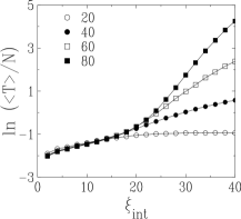
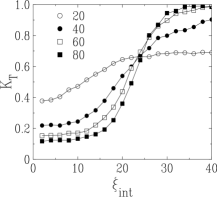
Figure 4: Top: logarithmic plot of the ratio $\langle T\rangle/N$ against $\xi_{\rm int}$, for a dynamical length $\xi_{\rm dyn}=\infty$, and variable column size $N$. Bottom: plot of the reduced variance $K_{T}$ against $\xi_{\rm int}$, for the same parameters.

The above intuitive picture is corroborated by Figure 4, showing a logarithmic plot of the ratio $\langle T\rangle/N$ and a plot of the reduced variance $K_{T}$ against $\xi_{\rm int}$, for several values of the column size $N$. There is evidence of a continuous phase transition between a ballistic phase for $\xi_{\rm int}<\xi_{{\rm int,}c}$ and an activated phase for $\xi_{\rm int}>\xi_{{\rm int,}c}$. We notice from the top panel that $\langle T\rangle/N$ is roughly independent of $N$ in the ballistic phase, whereas it grows fast with $N$ in the activated phase. On the other hand, the plots of $K_{T}$ approximately cross at a critical value $K_{T}\sim 0.7$ for $\xi_{\rm int}=\xi_{{\rm int,}c}\sim 26$.

This picture can be turned into the following effective model. We treat the thickness $L(t)$ as a collective coordinate, and model its dynamics by a biased Brownian motion on an interval, with velocity $V$ and diffusion constant $D$. The motion starts at time $t=0$ at an initial point $L(0)$ very near the free surface of the column, which is considered as a reflecting boundary. It ends at the random hitting time $t=T$ when $L(t)$ visits the base of the column, i.e., $L(t)=N$, for the first time. Accordingly, the base is considered as an absorbing boundary. This effective model is analysed in detail in Appendix B.

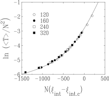
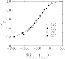
Figure 5: Top: logarithmic plot of $\langle T\rangle/N^{2}$ against $N(\xi_{\rm int}-\xi_{{\rm int,}c})$. for a dynamical length $\xi_{\rm dyn}=\infty$, $\xi_{{\rm int,}c}=28.4$, and variable $N$. Bottom: plot of the reduced variance $K_{T}$ against $X$, for the same parameters. Full lines: plots of the analytical results (B.31) and (B.32) for the effective model, rescaled according to (4.12).

Figure 5 shows that both the mean jamming time $\langle T\rangle$ and its reduced variance $K_{T}$ obey finite-size scaling laws of the form

$$\langle T\rangle\approx N^{2}\,F(X),\quad K_{T}\approx G(X),$$ (4.9)

with

$$X=N(\xi_{\rm int}-\xi_{{\rm int,}c}).$$ (4.10)

The best data collapse is obtained for

$$\xi_{{\rm int,}c}\approx 28.4.$$ (4.11)

Furthermore, the data are observed to be in accurate agreement with the finite-size scaling results (B.31) and (B.32), derived analytically in Appendix B for the effective model. The excellent quality of the accord suggests that the effective model predicts the exact finite-size scaling functions of the model. The best agreement, shown as full lines in Figure 5, is obtained with the following identification:

$$X\approx-115(z+3.4),\quad\ln(T_{0}/N^{2})\approx-4.3$$ (4.12)

between, on the empirical side, the scaling variable $X$ of the column model introduced in (4.10), and, on the theoretical side, the scaling variable

$$z=\displaystyle{\displaystyle VN\over\displaystyle D}$$ (4.13)

of the effective model, introduced in (B.30), and the diffusive time scale

$$T_{0}=\displaystyle{\displaystyle N^{2}\over\displaystyle 2D},$$ (4.14)

introduced in (B.24). This last relation, together with the second equation of (4.12), enable us to predict the critical value $D_{c}$ of the diffusion constant for $\xi_{\rm int}=\xi_{{\rm int,}c}$. We thus obtain $D_{c}\approx{\rm e}^{4.3}/2$, i.e.,

$$D_{c}\approx 37.$$ (4.15)

The reduced variance of the jamming time at the critical point is predicted in (B.26) to be a universal number:

$$K_{T}=\displaystyle{\displaystyle 2\over\displaystyle 3}.$$ (4.16)

This prediction is again in good agreement with the apparent crossing point of the data of the lower panel of Figure 4.

Finally, we compare the predictions of the effective model in the ballistic and activated phases with the above results.

$\bullet$ Toward the ballistic phase ($\xi_{\rm int}<\xi_{{\rm int,}c}$, i.e., $V>0$). In the ballistic phase, the prediction (B.21) for the mean jamming time:

$$\langle T\rangle\approx\displaystyle{\displaystyle N\over\displaystyle V}-\displaystyle{\displaystyle D\over\displaystyle V^{2}}$$ (4.17)

exhibits the observed ballistic behaviour (4.5), up to a finite negative correction due to diffusion.

The fluctuations of the jamming time around its mean are predicted to be Gaussian, with a reduced variance given by (B.22):

$$K_{T}\approx\displaystyle{\displaystyle 2D\over\displaystyle VN}.$$ (4.18)

This fall-off as $1/N$ agrees with the observation made above that fluctuations become relatively negligible for large columns.

The critical regime of the ballistic phase corresponds to the regime $X\to-\infty$, i.e., $z\to+\infty$, in the finite-size scaling laws (4.9). Equations (B.31) and (4.12) imply that the scaling function $F(X)$ falls off as $F(X)\approx A_{F}/\left|X\right|$, with $A_{F}\approx 115/D\approx 3.1$. This estimate implies in turn that the velocity vanishes linearly as $\xi_{\rm int}\to\xi_{{\rm int,}c}^{-}$, as $V\approx(\xi_{{\rm int,}c}-\xi_{\rm int})/A_{F}$, i.e.,

$$V\approx 0.32(\xi_{{\rm int,}c}-\xi_{\rm int}).$$ (4.19)

The numerical value of the prefactor is in good agreement with the slope of the extrapolation curve shown as a dashed line in Figure 3.

$\bullet$ Toward the activated phase ($\xi_{\rm int}>\xi_{{\rm int,}c}$, i.e., $V<0$). In the activated phase, the prediction (B.27) for the mean jamming time:

$$\langle T\rangle\approx\displaystyle{\displaystyle D\over\displaystyle V^{2}}\;{\rm e}^{\left|V\right|N/D}$$ (4.20)

grows exponentially with $N$, as anticipated in (4.8). The corresponding activation energy per unit length,

$$a=\displaystyle{\displaystyle\left|V\right|\over\displaystyle D},$$ (4.21)

is essentially given by the negative of the velocity. The reduced variance of the jamming time predicted by (B.29):

$$K_{T}\approx 1-\displaystyle{\displaystyle 2(VN+3D)\over\displaystyle D}\;{\rm e}^{-\left|V\right|N/D}$$ (4.22)

converges exponentially fast to its limiting value unity, characteristic of an exponential distribution.

The critical regime of the activated phase corresponds to the regime $X\to+\infty$, i.e., $z\to-\infty$, in the finite-scaling laws (4.9). The effective model predicts that the scaling function $G$ has an exponential convergence toward $G(+\infty)=1$, whereas the scaling function $F$ grows exponentially as $F\sim\exp(-z)\sim\exp(B_{F}X)$ with $B_{F}\approx 1/115\approx 0.0087$. These results corroborate our expectations, including (4.7) and (4.8). They also imply that the activation energy per grain vanishes linearly as $\xi_{\rm int}\to\xi_{{\rm int,}c}^{+}$, as $a(\xi_{\rm int})\approx B_{F}(\xi_{\rm int}-\xi_{{\rm int,}c})$, i.e.,

$$a(\xi_{\rm int})\approx 0.0087(\xi_{\rm int}-\xi_{{\rm int,}c}).$$ (4.23)

Before leaving this topic, we emphasise that the simple picture of a Brownian particle whose velocity $V$ changes sign at $\xi_{{\rm int,}c}$ appears to explain all our observations on this crossover.

Limiting behaviour for $\xi_{\rm int}\gg N$

We now look at the slowest possible dynamics in the activated phase; this will clearly occur when the column is at its most correlated, where $\xi_{\rm int}$ is much larger than $N$, still keeping $\xi_{\rm dyn}=\infty$ for simplicity. We are thus led to investigate the doubly singular limit where $\xi_{\rm dyn}=\xi_{\rm int}=\infty$. The only free parameter is then the column size $N$.

Figure 6: Top: logarithmic plot of the mean jamming time $\langle T\rangle$ against $N$, for $\xi_{\rm int}=\xi_{\rm dyn}=\infty$. Full line (hardly visible): fit $\langle T\rangle=N(\ln 2)/2-6.515\ln N+15.04$ to the data for $N>\xi_{{\rm int,}c}$. Bottom: plot of the reduced variance $K_{T}$ against $N$, for the same parameters. Arrows show the crossover scale $N=\xi_{{\rm int,}c}$ (see (4.11)).

Figure 6 shows plots of the mean jamming time $\langle T\rangle$ and of its reduced variance $K_{T}$ against $N$. When the column size $N$ is rather small, the system still behaves more or less ballistically; this fast dynamics leads to the nearly linear growth of $\langle T\rangle$ with $N$, and the concomitant decrease of the variance $K_{T}$ as a function of $N$. When $N$ is large enough, the system is fully activated, so that the jamming time grows exponentially with $N$, while the variance increases, rapidly converging to its asymptotic value $K_{T}=1$. The crossover between these behaviours occurs when the column size $N$ is of the order of $\xi_{{\rm int,}c}$ (shown as arrows in both plots).

Finally, we focus on the activation energy $a(\xi_{\rm int})$ defined in (4.8). When $\xi_{\rm int}\to\infty$, the column is at its most activated; hitting an attractor is then a totally random process. The jamming time is therefore expected to be simply given by the ratio between the number $\Omega_{0}=2^{N}$ of disordered initial configurations and the number $\Omega_{\infty}=2^{N/2}$ of possible attractors:

$$\langle T\rangle\sim\displaystyle{\displaystyle\Omega_{0}\over\displaystyle\Omega_{\infty}}\sim 2^{N/2}.$$ (4.24)

A similar purely entropic result is shown in Appendix C to hold within a toy model of a Markovian dynamics on an assembly of independent two-level systems. The result (4.24) implies that $a(\xi_{\rm int})$ saturates to the value

$$a_{\infty}=\displaystyle{\displaystyle\ln 2\over\displaystyle 2}\approx 0.34657.$$ (4.25)

This limiting value of the activation energy has been incorporated into the fit presented in the upper panel of Figure 6. The good quality of the fit can be viewed as corroborating the result (4.25), in spite of large correction terms.

To sum up, the activation energy $a(\xi_{\rm int})$ is expected to increase monotonically with $\xi_{\rm int}$ all over the activated phase, and to interpolate smoothly between the linear growth (4.23) as $\xi_{\rm int}\to\xi_{{\rm int,}c}^{+}$ (where the given numerical value of the prefactor only holds in the $\xi_{\rm dyn}\to\infty$ limit) and the purely entropic limiting value (4.25) as $\xi_{\rm int}\to\infty$.

4.3 Phase III (Logarithmic)

This phase of relatively small $\xi_{\rm int}$ and $\xi_{\rm dyn}$ is illustrated by panel III of Figure 1. The thickness $L(t)$ of the ordered layer follows a well-defined master curve, growing slower than linearly with time, again with relatively small fluctuations between different tracks.

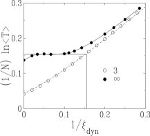
Figure 7: Plot of $(1/N)\ln\langle T\rangle$ against $1/\xi_{\rm dyn}$ for $N=50$. Empty symbols ($\xi_{\rm int}=3$) demonstrate the crossover between Phases I (ballistic) and III (logarithmic). Dashed line: prediction (4.28), with $V=6.95$. Full symbols ($\xi_{\rm int}=\infty$) corroborate the crossover (4.33) between Phases II (activated) and IV (glassy), in spite of large finite-size effects. Full straight lines: crossover at $1/\xi_{\rm dyn}\approx a_{\rm eff}\approx 0.155$ (see text).

Already encountered in the unhindered model III ; IV , this phenomenon can be explained as follows. Equation (4.4) shows that the application of zero-temperature dynamics causes order to propagate ballistically, for $\xi_{\rm int}<\xi_{{\rm int,}c}$ and $\xi_{\rm dyn}$ much larger than $N$. When $\xi_{\rm dyn}$ becomes comparable with $N$, however, grains move progressively slowly according to their depth, with local frequencies that scale as (2.3). Writing the differential equation

$${\displaystyle{\rm d}L\over\displaystyle{\rm d}t}\approx V\,\exp\left(-\displaystyle{\displaystyle L\over\displaystyle\xi_{\rm dyn}}\right),$$ (4.26)

we find that the thickness grows according to

$$L(t)\approx\xi_{\rm dyn}\ln\left(1+\displaystyle{\displaystyle Vt\over\displaystyle\xi_{\rm dyn}}\right).$$ (4.27)

and the mean jamming time for a column of size $N$ reads

$$\langle T\rangle\approx\displaystyle{\displaystyle\xi_{\rm dyn}\over\displaystyle V}\left(\exp\left(\displaystyle{\displaystyle N\over\displaystyle\xi_{\rm dyn}}\right)-1\right).$$ (4.28)

This result holds all over the left of the phase diagram of Figure 2 (Phases I and III and the crossover between them). It is confirmed quantitatively by the data shown (empty symbols) in Figure 7.

The laws (4.4) and (4.5) are recovered for $\xi_{\rm dyn}\gg N$, i.e., in the ballistic phase. In the logarithmic phase, when $\xi_{\rm dyn}\ll N$, the width of the ordered layer is predicted to grow logarithmically:

$$L(t)\approx\xi_{\rm dyn}\ln\displaystyle{\displaystyle Vt\over\displaystyle\xi_{\rm dyn}},$$ (4.29)

so that the mean jamming diverges exponentially fast with the column size $N$:

$$\langle T\rangle\approx\displaystyle{\displaystyle\xi_{\rm dyn}\over\displaystyle V}\,\exp\left(\displaystyle{\displaystyle N\over\displaystyle\xi_{\rm dyn}}\right).$$ (4.30)

4.4 Phase IV (Glassy)

The glassy phase is found when $\xi_{\rm int}$ is large and $\xi_{\rm dyn}$ is small; this is by far the richest and most novel phase of this model. The signal for $L(t)$, illustrated in panel IV of Figure 1, is neither nearly deterministic (as in the ballistic and logarithmic phases) nor totally random (as in the activated phase). The glassy phase corresponds to the ‘bottom’ of a long column, where grain reorientations are at their most hindered; grains in this region are weighed down by those above them and, additionally, feel to the fullest extent the effect of the orientational frustration between upper and lower grains.

This phenomenon is illustrated in Figure 8 from different viewpoints, using the time dependence of four observables (for the same stochastic history which was used to illustrate Phase IV in Figure 1). The jamming time $T\approx 279\,668$ for this history is about 2.4 times larger than the mean jamming time for the parameters $N=70$, $\xi_{\rm int}=50$, $\xi_{\rm dyn}=7$. The plotted observables are:

$\bullet$ the thickness $L(t)$ (see (4.3)) of the ordered upper layer,

$\bullet$ the second component ${\cal E}_{1}(t)$ (see (3.24)) of the pseudo-energy,

$\bullet$ the total number $\nu(t)$ of dimers,

$\bullet$ the fraction $\nu_{+-}(t)/\nu(t)$ of $(+-)$ dimers.

Figure 8: Top to bottom: plots of the thickness $L(t)$ of the ordered upper layer, the second component ${\cal E}_{1}(t)$ of the pseudo-energy, the numbers $\nu(t)$ of dimers, and the fraction $\nu_{+-}(t)/\nu(t)$ of $(+-)$ dimers, for the history illustrating Phase IV in Figure 1. Full symbols: values of the observables in the attractor, i.e., right at the jamming time $T$.

The last two quantities involve the following definitions of the numbers $\nu_{+-}$ of $(+-)$ dimers and $\nu_{-+}$ of $(-+)$ dimers:

$$\matrix{\displaystyle{\nu_{+-}={\textstyle{\displaystyle{\displaystyle 1\over\displaystyle 4}}}\sum_{k=2}^{N/2}(1+\sigma_{2k-1})(1-\sigma_{2k})},\hfill\cr\displaystyle{\nu_{-+}={\textstyle{\displaystyle{\displaystyle 1\over\displaystyle 4}}}\sum_{k=2}^{N/2}(1-\sigma_{2k-1})(1+\sigma_{2k})},\hfill\cr}$$ (4.31)

and of the total number $\nu=\nu_{+-}+\nu_{-+}$ of dimers in a given configuration:

$$\nu=\nu_{+-}+\nu_{-+}={\textstyle{\displaystyle{\displaystyle 1\over\displaystyle 2}}}\sum_{k=2}^{N/2}(1-\sigma_{2k-1}\sigma_{2k}).$$ (4.32)

The above formulae exclude the uppermost dimer, which is fixed by the boundary condition (2.12).

The four tracks shown in Figure 8 all show strongly correlated, intermittent and non-stationary fluctuations at all time scales, ranging from the instantaneous to scales of order of the jamming time $\langle T\rangle$ itself. These features are commonly observed in glassy systems. The existence of a glassy phase exhibiting this phenomenology in a one-dimensional model represents one of the most interesting outcomes of this work.

If we examine the dynamical history depicted in Figure 8, we will notice that it can be described as an alternation between two different kinds of periods:

$\bullet$ Periods of quietude. Four such periods are visible in the figure. They are characterised by quasi-stationary states with a high degree of order. The thickness $L(t)$ and the number $\nu(t)$ of dimers fluctuate around their maximal ground-state values of 70 and 34 respectively; the pseudo-energy ${\cal E}_{1}(t)$ is correspondingly minimised, and the fraction of $(+-)$ dimers is either close to zero or close to unity, indicating a highly polarised column which is close to one of the crystalline attractors $U_{\pm}$. In some sense, it is as if the system has almost made its mind up to choose one of the two global attractors, and is dawdling in its vicinity with nearly no major fluctuations, during each of these periods of quietude. However, these long excursions do not in any sense anticipate the fate of the column. In the given example, the attractor finally chosen (full symbol) is close to $U_{-}$, although the system spends most of its time in the vicinity of the attractor $U_{+}$ with the fraction of $(+-)$ dimers typically close to unity during the periods of quietude.

$\bullet$ Itinerant periods. During these periods of confused wandering between two consecutive periods of quietude, all the indicators fluctuate wildly with no particular aim in sight. All the observables monitored in Figure 8 are characterised by low order, with the pseudo-energy even going positive on occasion.

We end up with a speculation based on a pictorial analogy. The tracks in Figure 8 are reminiscent of those obtained in avalanche dynamics avalanches , where periods of small random events give rise to large system-size avalanches, which are known to be due to stress buildup and release on the surface. It is interesting, using this analogy, to speculate whether the itinerant periods in Figure 8 build up unsustainable geometric disorder all along the column, which can only be relieved by a systemic choice of a nearly ordered configuration (that is close to an attractor), in which the column then lives, until disorder strikes again in the form of the next itinerant period.

Mean jamming time

We now focus on a quantitative analysis of several aspects of the glassy phase, beginning with the mean jamming time $\langle T\rangle$. Recall that in the activated phase, i.e., for $\xi_{\rm int}>\xi_{{\rm int,}c}$ and $\xi_{\rm dyn}$ large enough, the jamming time grows exponentially fast with $N$ (see (4.8)). We now examine the effect of decreasing $\xi_{\rm dyn}$, to cross over into the glassy phase.

The main effect of this is that an increasingly broad spectrum of local frequency scales $\omega_{n}$ kicks in, to slow down the stochastic behaviour of the activated phase. Interestingly, a toy model of an assembly of independent two-level systems is able to provide a clue to this crossover. Its details are presented in Appendix C, but the crucial feature is that it has two regimes – one where entropy dominates (‘entropic’), and the other which is dominated by the slowest of the local frequencies (‘slow’).

The mean jamming time is in fact what would be most naively expected from the above competition, that is, it is the greater of the two times that would be generated:

$$\langle T\rangle\sim{\rm max}\,\Bigl{(}\exp(a(\xi_{\rm int})N),\;\exp(N/\xi_{\rm dyn})\Bigr{)},$$ (4.33)

where $\exp(a(\xi_{\rm int})N)$ is the jamming time of (4.8) in the $\xi_{\rm dyn}\to\infty$ limit, while $1/\omega_{N}=\exp(N/\xi_{\rm dyn})$ is the slowest microscopic time scale of the problem. More specifically, this implies the following:

$\bullet$ In the activated phase, when $\xi_{\rm dyn}>1/a(\xi_{\rm int})$, the result (4.8) for the mean jamming time in the $\xi_{\rm dyn}\to\infty$ limit is essentially unchanged – this corresponds to the entropic phase of the toy model of Appendix C.

$\bullet$ In the glassy phase, i.e., for $\xi_{\rm dyn}<1/a(\xi_{\rm int})$, the jamming time grows proportionally to $1/\omega_{N}=\exp(N/\xi_{\rm dyn})$ – this corresponds to the slow phase of the toy model of Appendix C.

From the above, one naturally expects there to be a sharp transition in the $\xi_{\rm int}-\xi_{\rm dyn}$ plane, along the line defined by

$$\xi_{\rm dyn}(\xi_{\rm int})=\displaystyle{\displaystyle 1\over\displaystyle a(\xi_{\rm int})},$$ (4.34)

shown qualitatively in Figure 2. For the strongest correlations, as $\xi_{\rm int}\to\infty$, the transition point $\xi_{\rm dyn}(\xi_{\rm int})$ takes its minimum value $\xi_{\rm dyn}(\infty)=1/a_{\infty}=2/(\ln 2)\approx 2.8854$ (see (4.25)). On the other hand, at the boundary of the ballistic/logarithmic and activated regimes ($\xi_{\rm int}\to\xi_{{\rm int,}c}^{+}$), (4.23) predicts a divergence of the transition point of the form

$$\xi_{\rm dyn}(\xi_{\rm int})\approx 115/(\xi_{\rm int}-\xi_{{\rm int,}c}).$$ (4.35)

Despite huge finite-size effects, our simulation data (shown as full symbols in Figure 7) manifest the crossover described above. The plateau in the left part of the data (full horizontal line) yields the effective value $a_{\rm eff}\approx 0.155$ for $\xi_{\rm int}=\infty$ and $N=50$. This effective value is very far from the theoretical asymptotic value $a_{\infty}$ (see (4.25)), underlining the importance of finite-size effects. However, and reassuringly for our analysis, the crossover does indeed take place as predicted by (4.34), at a value of $1/\xi_{\rm dyn}\approx a_{\rm eff}$ (full vertical line).

Statistics of attractors

We now turn to the statistics of attractors in the glassy phase. The question of what they are is easily addressed. Recall that the ground states of the model for $\varepsilon=1$ are the $2^{\nu}$ configurations made up of $\nu=N/2-1$ dimers, which satisfy the boundary condition (2.12). By construction, these are the possible attractors of zero-temperature dynamics.

The next question, which relates to their dynamical attainability, is less easy to answer. A precise formulation of this question is: What is the probability $Q({\cal C})$ that the application of zero-temperature dynamics leaves the column in a given attractor ${\cal C}$, starting from a uniformly chosen random initial configuration? Or, more physically: how and where does a constrained system, starting from random initial conditions, attain jamming? This question has held centre stage in theoretical compcoop ; gl and experimental sidnature explorations of granular media and many other complex systems, ever since Edwards postulated that the entropic landscape of granular systems was flat edwards . Edwards’ flatness hypothesis (in the strong sense) implies that the attractors are sampled uniformly by the dynamics, so that $Q({\cal C})$ is independent of the attractor ${\cal C}$, and therefore equal to the reciprocal of the total number of attractors.

Our reason for introducing these issues at such a late stage in this paper is that the statistics of attractors are likely to be non-trivial only in the glassy phase. All the other phases indeed manifest sufficiently stochastic behaviour that one would expect the entropic landscape to be at least approximately flat.

A central quantity in this framework is therefore the dynamical entropy

$$S=-\sum_{\cal C}Q({\cal C})\ln Q({\cal C}).$$ (4.36)

In the case where the attractors are sampled uniformly, according to Edwards’ hypothesis, the dynamical entropy assumes its maximal value:

$$S_{\rm max}=\nu\ln 2,$$ (4.37)

where $\nu=N/2-1$.

Measuring entropies directly via numerical simulations is known to be a very difficult task. Instead, we resort to an inspired guess. Since it seems likely that the crystalline attractors $U_{\pm}$ introduced in (3.21) will play a special role in the dynamics, we use them implicitly to define quantities of interest on the attractors reached by the dynamics:

$\bullet$ A global indicator is provided by the probability distribution $p(\nu_{+-})$ of the number of $(+-)$ dimers. By using the dimer variables $\eta_{k}$ introduced in (3.19), the definitions (4.31) can be simplified as:

$$\nu_{+-}={\textstyle{\displaystyle{\displaystyle 1\over\displaystyle 2}}}\sum_{k=2}^{N/2}(1+\eta_{k}),\quad\nu_{-+}={\textstyle{\displaystyle{\displaystyle 1\over\displaystyle 2}}}\sum_{k=2}^{N/2}(1-\eta_{k}),$$ (4.38)

so that $\nu_{+-}+\nu_{-+}=\nu=N/2-1$.

If Edwards’ hypothesis holds, i.e., if the $2^{\nu}$ attractors are all equally likely to occur as attractors, the distribution of $\nu_{+-}$ is binomial:

$$p(\nu_{+-})=\displaystyle{\displaystyle 1\over\displaystyle 2^{\nu}}{\nu\choose\nu_{+-}}=\displaystyle{\displaystyle\nu!\over\displaystyle 2^{\nu}(\nu_{+-})!(\nu_{-+})!}.$$ (4.39)

In such a binomial distribution, the extremal values $\nu_{+-}=0$ and $\nu_{+-}=\nu$, corresponding to the crystalline attractors $U_{\pm}$ (where all the dimers are of the same kind) are the least probable. On the other hand, if the actual distributions obtained deviate from the binomial law (4.39), this would indicate strongly that all the attractors are not equally likely, the entropic landscape is not flat, and thus of course that Edwards’ hypothesis does not hold.

$\bullet$ A local indicator of attractor structure is the correlation function

$$\chi_{k}=\displaystyle{\displaystyle\langle(\nu_{+-}-\nu_{-+})\eta_{k}\rangle-1\over\displaystyle\nu-1}.$$ (4.40)

This correlation measures the trend for the $k$-th dimer to be aligned with every other dimer. It vanishes identically if Edwards’ flatness hypothesis holds. In the extreme opposite situation where only the crystalline attractors $U_{\pm}$ are reached by the dynamics, the above correlation takes its maximal value $\chi_{k}=1$ for all $k$.

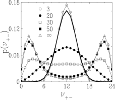
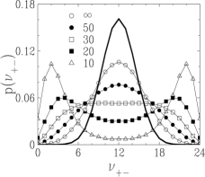
Figure 9: Histogram plots of the probability distribution $p(\nu_{+-})$ for $N=50$ (hence $\nu=24$). Top: $\xi_{\rm dyn}=10$ and variable $\xi_{\rm int}$. Bottom: $\xi_{\rm int}=\infty$ and variable $\xi_{\rm dyn}$. The binomial distribution (4.39) is shown as thick full lines.

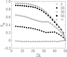
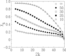
Figure 10: Plot of the dimer correlation function $\chi_{k}$ against depth $n=2k$. Parameters are as in Figure 9.

Our numerical results for the probability distribution $p(\nu_{+-})$ and the dimer correlation function $\chi_{k}$ are shown in Figures 9 and 10. All the data were taken for a system of size $N=50$, which has $\nu=24$ dimers that are free to reorient. Figure 9 shows the variation of the form of $p(\nu_{+-})$ with, first, fixed $\xi_{\rm dyn}=10$ and variable $\xi_{\rm int}$, and next, fixed $\xi_{\rm int}=\infty$ and variable $\xi_{\rm dyn}$. Figure 10 shows the variation of $\chi_{k}$ along the same diagnostic lines.

In Figure 9, the binomial distribution (corresponding to Edwards’ flatness hypothesis) is shown by a thick full line, with which the data for the lowest value of $\xi_{\rm int}$ are almost completely aligned. The statistics of attractors is thus very close to being uniform in the ballistic and logarithmic phases, which correspond to the top layers of a column. As $\xi_{\rm int}$ increases, there is a gradual crossover to a non-trivial two-peaked distribution; the same trend is visible in the lower panel, when $\xi_{\rm dyn}$ decreases for infinite $\xi_{\rm int}$. At the beginning of the crossover, with its small deviations from uniform sampling, one recognises the activated phase, which corresponds to the middle of a column. By the time that the two-peaked distribution is obtained in both parts of Figure 9, the parameters – $\xi_{\rm int}$ large, and $\xi_{\rm dyn}$ small – correspond clearly to the glassy phase. Here, attractors in the neighbourhoods of the crystalline states $U_{\pm}$ are eventually favoured, after long periods of systemic wandering.

The above observations are reinforced by Figure 10. In the upper panel, the correlation function $\chi_{k}$ is essentially zero for low $\xi_{\rm int}$, increasing progressively as $\xi_{\rm int}$ is increased. In the lower panel, i.e., for infinite $\xi_{\rm int}$, the correlation function is never quite zero even for high $\xi_{\rm dyn}$, and only manifests a stronger depth-dependence as $\xi_{\rm dyn}$ decreases. These results reinforce those found in an independent model which uses random graphs to model grains near jamming, where entropic deviations from Edwards’ flatness occur in certain regions of parameter space johannes .

To recapitulate, the salient feature that emerges is that the system prefers increasingly to live in the neighbourhood of its two global minima, the attractors $U_{\pm}$, as one goes deep into the glassy phase. As a consequence, the dynamical entropy decreases from a value close to its maximal value (4.37) at the boundary between Phases II and IV, to zero in the deepest part of the glassy phase ($\xi_{\rm int}\gg N$, $\xi_{\rm dyn}\ll N$). Furthermore, Edwards’ flatness is well obeyed overall in three out of four phases in this model; it is massively violated only deep in the glassy phase of this model, where the configurational landscape is completely rough.

Our success in constructing this glassy phase via such a minimal model relied on the inclusion of two crucial ingredients:

$\bullet$ Long-range interactions ($\xi_{\rm int}>N$), in order for the dimers to jam cooperatively, rather than independently of each other;

$\bullet$ A broad spectrum of local frequencies ($\xi_{\rm dyn}$ small) to slow down the relaxation, and thus prevent a purely activated mechanism driven by entropy.

It is noteworthy that both these minimal ingredients rely on collective effects – one to do with interactions in space, the other to do with degrees of freedom in time. This model-specific conclusion at once agrees with, and reinforces, general notions miguel of cooperativity in glassy dynamics.

5 Discussion

The motivation for this model came from a mental image of grains in a box under shaking: what could be at once so simple, or – as we came to see in time – so complex? Our first, simplest, model I ; II involved only the effects of gravity on non-interacting grains – deeper grains carried the weight of grains above them, so were less free to move. This was modelled by using a single dynamical length $\xi_{\rm dyn}$, representing the thickness of the dynamical boundary layer: grains at a depth $n$ much less than $\xi_{\rm dyn}$ (which can be examined by setting $\xi_{\rm dyn}\to\infty$) are free to move, whereas those where $n\sim\xi_{\rm dyn}$ have lower frequencies of motion, as normal in non-Newtonian fluids. Three phases were found; in the ‘fluidised’ phase, grains flew as well as moved along the surface, with a relatively quick propagation of order down the sandbox. Grain disorder was essentially frozen in, in the ‘glassy’ phase, with a very slow propagation of order from the free surface. The ‘intermediate’ phase was in some ways the most interesting, with a true competition between fast and slow dynamics.

In hindsight, it is astonishing that these diverse behaviours – especially the shape-dependent ‘ageing’ effects of the glassy regime – were manifested in a totally non-interacting model. A more realistic, interacting model of the glassy regime was presented in III ; IV . Since close-packed grains can typically not diffuse spatially, it was sufficient to model a column, rather than a box, of grains. In the model of III ; IV , grain motions were constrained not just by the masses, but also by the orientations of grains above them, thus generating directional long-range interactions. The effect of compaction around jamming was modelled by a single local field $h_{n}$, representing the excess void space br for grain $n$, which could be minimised by a suitable choice of grain orientation. Additionally, in this model, grains were allowed to have arbitrary shapes, so that the the disordered orientation of a grain could occupy any volume $\varepsilon$, and, correspondingly generate any void space. The propagation of order in this model proceeded from the free surface to the base, and was ‘causal in space’ – in that while upper grains constraint lower ones, the converse was not true.

It took us some time and several explorations to realise that while the model of III ; IV had at least the flavour of the interactions needed to model a jammed glassy phase – e.g. the constraining effect of long-range grain correlations – its lack of slow dynamics (except those arising from the trivial effect of grain masses) was a direct result of its spatial causality. Essentially, provided a grain was not blocked down by the weight of other grains, it was free to orient itself subject only to the orientations of grains above itself – that is, we were modelling the behaviour of the top layers of a jammed column of grains, which never felt the undertow of the base. It was small surprise, therefore, that the ordering dynamics for $\xi_{\rm dyn}\to\infty$ were ballistic.

To model a column of grains with spatial inhomogeneities – that is, a column with a top, a middle, and a bottom – we discovered that orientational constraints needed to be inserted in a non-directed way. This enabled us to model frustration – in this context, the need of a given grain to balance the effects of two competing local fields $h_{n}$ and $j_{n}$ – which led in its turn, to slow dynamics. Still keeping the orientational constraints of previous models I ; II ; III ; IV via the field $h_{n}$, as well as the effect of ‘gravitational slowing down’ via $\xi_{\rm dyn}$, we therefore introduced here the notion that grains were also constrained by grains below them, via the field $j_{n}$ which propagated over a correlation length $\xi_{\rm int}$.

From this very heuristic and pictorial modelling has emerged a model column of grains that manifests all the complexity of earlier models III ; IV , and adds some more via the introduction of the activated and glassy phases. Our main success is of course in the realisation of a glassy phase for which a minimal combination of two physical ingredients – strong, bi-directional, orientational correlations and a broad spectrum of local frequencies arising from a natural depth-dependence – appears to be necessary. The richness of this phase is worthy of further exploration, especially to do with issues concerning higher-order correlations and ageing.

Finally, we mention that our model provides some rather interesting and general insights into the nature of optimisation – the granular column modelled here reaches its ground states in strikingly different ways, in the four dynamical phases mentioned above. It is tempting to think of these phases as representing different spatial parts – ‘top’, ‘middle’ and ‘bottom’ – of a column, and to connect their different routes to compaction with the issue of inhomogeneities in real granular media . While this picture is an appealing one, one should remember that the four phases of this model were obtained by varying $\xi_{\rm int}$ and $\xi_{\rm dyn}$; the translation of our results to apply to a real column would involve the natural apparition of such variations as a function of depth.

Appendix A. Exact results for $N=4$ and $N=6$

In this Appendix we derive analytical results on the zero-temperature dynamics of the model investigated in the body of the paper, for small systems. We concentrate onto the statistics of attractors, i.e., the probability that the system is absorbed in each attractor, starting from a random initial configuration. Exact results will be successively obtained for systems of sizes $N=4$ and $N=6$, for arbitrary $\xi_{\rm int}$ and $\xi_{\rm dyn}$.

The case $N=4$

The column made of 4 grains with the boundary condition (2.12) has three free orientations : $\sigma_{2}\pm 1$, $\sigma_{3}=\pm 1$, $\sigma_{4}=\pm 1$, and therefore eight configurations, in lexicographical order:

$$\matrix{{\cal C}_{1}=++++,\quad{\cal C}_{2}={+++-},\quad{\cal C}_{3}=++-+,\hfill\cr{\cal C}_{4}=++--,\quad{\cal C}_{5}={+-++},\quad{\cal C}_{6}=+-+-,\hfill\cr{\cal C}_{7}=+--+,\quad{\cal C}_{8}={+---}.\hfill}$$ (A.1)

The two attractors are the dimerised configurations ${\cal C}_{6}$ and ${\cal C}_{7}$, respectively corresponding to $\eta_{2}=+1$ and $\eta_{2}=-1$. Our main goal is to determine the probabilities $Q^{(6)}$ and $Q^{(7)}$ that the system is absorbed in each of these attractors, starting from a random initial configuration. The relevant information is encoded in the non-uniformity parameter

$$\Delta=\langle\eta_{2}\rangle=Q^{(6)}-Q^{(7)}.$$ (A.2)

The zero-temperature dynamics consists of a certain number of moves between configurations. For instance, ${\cal C}_{1}$ may be updated into the following configurations at the following rates:

$${\cal C}_{1}\mathrel{\mathop{\longrightarrow}\limits^{\omega_{2}}}{\cal C}_{5},\quad{\cal C}_{1}\mathrel{\mathop{\longrightarrow}\limits^{\omega_{3}}}{\cal C}_{3},\quad{\cal C}_{1}\mathrel{\mathop{\longrightarrow}\limits^{\omega_{4}}}{\cal C}_{2}.$$ (A.3)

As announced in Section 3.3, this dynamics is independent of $\xi_{\rm int}$ for $N=4$. It can be represented as an $8\times 8$ Markov matrix ${\bf M}$, such that the occupation probabilities $P_{a}(t)$ of the configurations ${\cal C}_{a}$ ($a=1,\dots,8$) obey the forward Kolmogorov equation redner ; feller

$${\displaystyle{\rm d}P_{a}(t)\over\displaystyle{\rm d}t}=\sum_{b}{\bf M}_{ab}P_{b}(t).$$ (A.4)

The absorption probabilities of the attractors can be derived by means of the following approach. Let $Q^{(c)}_{a}$ be the probability of being eventually absorbed by configuration ${\cal C}_{c}$, starting from the initial configuration ${\cal C}_{a}$. For a fixed configuration ${\cal C}_{c}$, the absorption probabilities $Q^{(c)}_{a}$ obey the backward Kolmogorov equation redner ; feller

$$\sum_{a}Q^{(c)}_{a}{\bf M}_{ab}=0,$$ (A.5)

complemented by the boundary condition $Q^{(c)}_{c}=1$. For a random initial configuration, we have therefore

$$Q^{(c)}=\displaystyle{\displaystyle 1\over\displaystyle 8}\sum_{a}Q^{(c)}_{a}.$$ (A.6)

By solving (A.5) successively for both attractors ($c=6$ and $c=7$), we are left with the following explicit result, for arbitrary rates $\omega_{n}$:

$$\Delta=\displaystyle{\displaystyle\omega_{3}\omega_{4}(\omega_{3}-\omega_{4})\over\displaystyle 2(\omega_{2}+\omega_{3})(\omega_{2}+\omega_{4})(\omega_{3}+\omega_{4})}.$$ (A.7)

In the present model, where $\omega_{n}=x_{\rm dyn}^{n}$ (see (2.3)), this result simplifies to

$$\Delta=\displaystyle{\displaystyle(1-x_{\rm dyn})x_{\rm dyn}^{3}\over\displaystyle 2(1+x_{\rm dyn})^{2}(1+x_{\rm dyn}^{2})}.$$ (A.8)

The non-uniformity parameter $\Delta$ is a small positive quantity, meaning that the crystalline attractor ${\cal C}_{6}=U_{+}$ is always slightly favoured by the dynamics. It coincides with $\Delta_{1}$ plotted in the upper panel of Figure 11. It vanishes in both limits $x_{\rm dyn}\to 0$ (i.e., $\xi_{\rm dyn}\to 0$) and $x_{\rm dyn}\to 1$ (i.e., $\xi_{\rm dyn}\to\infty$). Its maximum $\Delta\approx 0.012465$ is reached for $x_{\rm dyn}\approx 0.6253$.

The case $N=6$

The case of a column made of $N=6$ grains can still be dealt with by analytical means, although the final expressions are much lengthier. The system has 32 configurations. Its four attractors are the following configurations (relabelled as $a=1,\dots,4$ for convenience):

$$\matrix{{\cal C}_{1}=+-+-+-,\quad{\cal C}_{2}=+-+--+,\hfill\cr{\cal C}_{3}=+--++-,\quad{\cal C}_{4}=+--+-+.\hfill}$$ (A.9)

The relevant information is encoded in the three non-uniformity parameters

$$\matrix{\Delta_{1}=\langle\eta_{2}\rangle=Q^{(1)}+Q^{(2)}-Q^{(3)}-Q^{(4)},\hfill\cr\Delta_{2}=\langle\eta_{3}\rangle=Q^{(1)}-Q^{(2)}+Q^{(3)}-Q^{(4)},\hfill\cr\Delta_{3}=\langle\eta_{2}\eta_{3}\rangle=Q^{(1)}-Q^{(2)}-Q^{(3)}+Q^{(4)}.\hfill}$$ (A.10)

As announced in Section 3.3, $N=6$ is the smallest system size such that the dynamics depends in a non-trivial way on the parameter $\xi_{\rm int}$. The Markov matrix ${\bf M}$ assumes two different expressions for $0<x_{\rm int}<\phi$ and $\phi<x_{\rm int}<1$, where the inverse golden mean $\phi$ is given in (3.15). For each of these two phases, the $32\times 32$ Markov matrix ${\bf M}$ has been generated, and the backward equations (A.5) corresponding to each of the four attractors have been solved analytically. We thus obtain the following expressions for the non-uniformity parameters, in the range $0<x_{\rm int}<\phi$:

$$\matrix{\Delta_{1}=\displaystyle{\displaystyle(1-x_{\rm dyn})x_{\rm dyn}^{3}\over\displaystyle 2(1+x_{\rm dyn})^{2}(1+x_{\rm dyn}^{2})},\hfill\cr\Delta_{2}=(x_{\rm dyn}^{4}-1)(x_{\rm dyn}^{3}+x_{\rm dyn}^{2}+1)\hfill\cr{\hskip 14.22636pt}\times(x_{\rm dyn}^{4}+x_{\rm dyn}^{3}+x_{\rm dyn}^{2}+1)x_{\rm dyn}^{6}\displaystyle{\displaystyle P_{24}(x_{\rm dyn})\over\displaystyle D(x_{\rm dyn})},\hfill\cr\Delta_{3}=-(x_{\rm dyn}-1)^{2}(x_{\rm dyn}^{2}+1)(x_{\rm dyn}^{3}+x_{\rm dyn}^{2}+1)\hfill\cr{\hskip 14.22636pt}\times(x_{\rm dyn}^{4}+x_{\rm dyn}^{3}+x_{\rm dyn}^{2}+1)x_{\rm dyn}^{5}\displaystyle{\displaystyle P_{25}(x_{\rm dyn})\over\displaystyle D(x_{\rm dyn})},\hfill}$$ (A.11)

and in the range $\phi<x_{\rm int}<1$:

$$\matrix{\Delta_{1}=-x_{\rm dyn}^{3}\displaystyle{\displaystyle P_{38}(x_{\rm dyn})\over\displaystyle D(x_{\rm dyn})},\hfill\cr\Delta_{2}=(x_{\rm dyn}^{4}-1)(x_{\rm dyn}^{3}+x_{\rm dyn}^{2}+1)\hfill\cr{\hskip 14.22636pt}\times(x_{\rm dyn}^{4}+x_{\rm dyn}^{3}+x_{\rm dyn}^{2}+1)x_{\rm dyn}^{6}\displaystyle{\displaystyle P_{24}(x_{\rm dyn})\over\displaystyle D(x_{\rm dyn})},\hfill\cr\Delta_{3}=(1-x_{\rm dyn}^{4})(x_{\rm dyn}^{3}+x_{\rm dyn}^{2}+1)\hfill\cr{\hskip 14.22636pt}\times(x_{\rm dyn}^{4}+x_{\rm dyn}^{3}+x_{\rm dyn}^{2}+1)\displaystyle{\displaystyle P_{30}(x_{\rm dyn})\over\displaystyle D(x_{\rm dyn})},\hfill}$$ (A.12)

where we have introduced the following polynomials:

$${\hskip-10.81204pt}\matrix{{\hskip 6.54413pt}D(x)=8(x+1)^{3}(x^{2}+1)^{2}(x^{2}-x+1)(x^{2}+x+1)^{2}\hfill\cr{\hskip 29.30634pt}\times(x^{3}+x+1)^{2}(x^{3}+x^{2}+1)^{2}(x^{4}+x^{2}+x+1)\hfill\cr{\hskip 29.30634pt}\times(x^{4}+x+1)(x^{4}+x^{3}+1)(x^{4}+x^{3}+x^{2}+1),\hfill}$$ (A.13)

$${\hskip-15.07996pt}\matrix{P_{24}(x)=4x^{24}+5x^{23}+10x^{22}+15x^{21}+9x^{20}-5x^{19}\hfill\cr{\hskip 29.30634pt}-51x^{18}-104x^{17}-203x^{16}-308x^{15}-434x^{14}\hfill\cr{\hskip 29.30634pt}-515x^{13}-605x^{12}-634x^{11}-609x^{10}-533x^{9}\hfill\cr{\hskip 29.30634pt}-449x^{8}-330x^{7}-218x^{6}-130x^{5}-71x^{4}\hfill\cr{\hskip 29.30634pt}-27x^{3}-3x^{2}+x+1,\hfill}$$ (A.14)

$$\matrix{P_{25}(x)=6x^{25}+15x^{24}+40x^{23}+95x^{22}+185x^{21}\hfill\cr{\hskip 29.30634pt}+335x^{20}+547x^{19}+842x^{18}+1177x^{17}+1556x^{16}\hfill\cr{\hskip 29.30634pt}+1900x^{15}+2193x^{14}+2349x^{13}+2356x^{12}\hfill\cr{\hskip 29.30634pt}+2223x^{11}+1955x^{10}+1609x^{9}+1242x^{8}+888x^{7}\hfill\cr{\hskip 29.30634pt}+590x^{6}+367x^{5}+207x^{4}+101x^{3}+43x^{2}\hfill\cr{\hskip 29.30634pt}+17x+4,\hfill}$$ (A.15)

$${\hskip-9.95845pt}\matrix{P_{30}(x)=6x^{30}+21x^{29}+54x^{28}+140x^{27}+292x^{26}\hfill\cr{\hskip 29.30634pt}+546x^{25}+949x^{24}+1531x^{23}+2283x^{22}\hfill\cr{\hskip 29.30634pt}+3207x^{21}+4277x^{20}+5377x^{19}+6457x^{18}\hfill\cr{\hskip 29.30634pt}+7343x^{17}+8025x^{16}+8316x^{15}+8236x^{14}\hfill\cr{\hskip 29.30634pt}+7793x^{13}+7011x^{12}+5978x^{11}+4852x^{10}\hfill\cr{\hskip 29.30634pt}+3730x^{9}+2682x^{8}+1811x^{7}+1142x^{6}+662x^{5}\hfill\cr{\hskip 29.30634pt}+343x^{4}+160x^{3}+64x^{2}+20x+4,\hfill}$$ (A.16)

$${\hskip-1.42262pt}\matrix{P_{38}(x)=4x^{38}+28x^{37}+109x^{36}+341x^{35}+909x^{34}\hfill\cr{\hskip 29.30634pt}+2114x^{33}+4416x^{32}+8424x^{31}+14836x^{30}\hfill\cr{\hskip 29.30634pt}+24262x^{29}+37105x^{28}+53309x^{27}+72124x^{26}\hfill\cr{\hskip 29.30634pt}+92105x^{25}+111177x^{24}+127001x^{23}\hfill\cr{\hskip 29.30634pt}+137190x^{22}+140074x^{21}+135038x^{20}\hfill\cr{\hskip 29.30634pt}+122612x^{19}+104406x^{18}+82925x^{17}+60963x^{16}\hfill\cr{\hskip 29.30634pt}+40790x^{15}+24131x^{14}+11829x^{13}+3799x^{12}\hfill\cr{\hskip 29.30634pt}-720x^{11}-2614x^{10}-2891x^{9}-2404x^{8}-1693x^{7}\hfill\cr{\hskip 29.30634pt}-1031x^{6}-555x^{5}-269x^{4}-112x^{3}-39x^{2}\hfill\cr{\hskip 29.30634pt}-11x-2.\hfill}$$ (A.17)

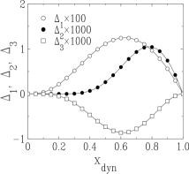
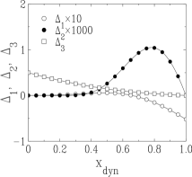
Figure 11: Plots of the non-uniformity parameters $\Delta_{i}$ ($i=1,2,3$) characterising the attractor statistics of a column of $N=6$ grains. Top: $0<x_{\rm int}<\phi$ (see (A.11)). Bottom: $\phi<x_{\rm int}<1$ (see (A.12)). Note the powers of 10 in the vertical scales.

The non-uniformity parameters $\Delta_{i}$ are plotted in Figure 11 (note the powers of 10 in the vertical scales). For $0<x_{\rm int}<\phi$ (upper panel), the $\Delta_{i}$ are typically small. They vanish in both limits $x_{\rm dyn}\to 0$ and $x_{\rm dyn}\to 1$. $\Delta_{1}$ is always positive, and it coincides with $\Delta$ of the case $N=4$ (see (A.8)); $\Delta_{2}$ turns from negative to positive for $x_{\rm dyn}\approx 0.2598$, whereas $\Delta_{3}$ is always negative. For $\phi<x_{\rm int}<1$ (lower panel), the $\Delta_{i}$ are typically larger. Only $\Delta_{2}$ is the same in both phases. The $\Delta_{i}$ again vanish in both limits $x_{\rm dyn}\to 0$ and $x_{\rm dyn}\to 1$, except for $\Delta_{1}=-5/96$ for $x_{\rm dyn}=1$ and $\Delta_{3}=1/2$ for $x_{\rm dyn}=0$. Finally, $\Delta_{1}$ turns from positive to negative for $x_{\rm dyn}\approx 0.6581$, whereas $\Delta_{3}$ is always positive.

Appendix B. Biased Brownian motion on an interval

In this appendix we consider biased Brownian motion on the interval $0<x<L$, characterised by its drift velocity $V$ and its diffusion coefficient $D$. The endpoint at $x=0$ is reflecting, whereas the endpoint at $x=L$ is absorbing.

This mixed type of boundary conditions is referred to as the transmission mode redner . It ensures that, starting at a given position $x=\ell$, the particle hits the absorbing endpoint with certainty in some finite random time $T$, referred to as the absorption time. Our main goal is to determine the distribution $\rho(T)$ of this absorption time, and especially its first few moments. We shall mostly concentrate onto the $\ell\to 0$ limit, where the particle starts from the immediate vicinity of the reflecting endpoint.

Let $P(x,t)$ be the probability density for the particle to be at point $x$ at time $t$, and $J(x,t)$ the associated probability current. We have

$${\displaystyle\partial P\over\displaystyle\partial t}+\displaystyle{\displaystyle\partial J\over\displaystyle\partial x}=0,\quad J=VP-D\,\displaystyle{\displaystyle\partial P\over\displaystyle\partial x},$$ (B.1)

with the initial and boundary conditions

$$P(x,0)=\delta(x-\ell),\quad J(0,t)=P(L,t)=0.$$ (B.2)

Introducing the Laplace transform

$$\widehat{P}(x,s)=\int_{0}^{\infty}P(x,t)\,{\rm e}^{-st}\,{\rm d}t,$$ (B.3)

the above equations imply

$$s\widehat{P}+V\,\displaystyle{\displaystyle\partial\widehat{P}\over\displaystyle\partial x}-D\,\displaystyle{\displaystyle\partial^{2}\widehat{P}\over\displaystyle\partial x^{2}}=\delta(x-\ell),$$ (B.4)

with boundary conditions

$$V\widehat{P}(0,s)-D\,\displaystyle{\displaystyle\partial\widehat{P}(0,s)\over\displaystyle\partial x}=\widehat{P}(L,s)=0.$$ (B.5)

Equation (B.4) implies the matching conditions

$$\matrix{\widehat{P}(\ell^{+},s)=\widehat{P}(\ell^{-},s),\hfill\cr\displaystyle{\displaystyle\partial\widehat{P}(\ell^{+},s)\over\displaystyle\partial x}-\displaystyle{\displaystyle\partial\widehat{P}(\ell^{-},s)\over\displaystyle\partial x}=-\displaystyle{\displaystyle 1\over\displaystyle D}.}$$ (B.6)

Consider first the homogeneous equation obtained by setting the right-hand side of (B.4) equal to zero. Looking for a solution to this equation at fixed $s$ of the form $\widehat{P}={\rm e}^{rx}$, we obtain the quadratic equation $s+Vr-Dr^{2}=0$, whose two roots read

$$r_{1}=\displaystyle{\displaystyle V-W\over\displaystyle 2D},\quad r_{2}=\displaystyle{\displaystyle V+W\over\displaystyle 2D},\quad W=(V^{2}+4Ds)^{1/2}.$$ (B.7)

The solution obeying the boundary conditions (B.5) reads

$$\widehat{P}(x,s)=\left\{\matrix{A(r_{1}\,{\rm e}^{r_{1}x}-r_{2}\,{\rm e}^{r_{2}x})\hfill&(0<x<\ell),\hfill\cr\cr B({\rm e}^{r_{1}(x-L)}-{\rm e}^{r_{2}(x-L)})\hfill&(\ell<x<L).\hfill}\right.$$ (B.8)

Finally, the constants $A$ and $B$ are determined from the matching conditions (B.6):

$$\matrix{A=\displaystyle{\displaystyle{\rm e}^{-r_{1}\ell-r_{2}L}-{\rm e}^{-r_{2}\ell-r_{1}L}\over\displaystyle D(r_{2}-r_{1})(r_{2}\,{\rm e}^{-r_{1}L}-r_{1}\,{\rm e}^{-r_{2}L})},\hfill\cr B=\displaystyle{\displaystyle r_{2}\,{\rm e}^{-r_{1}\ell}-r_{1}\,{\rm e}^{-r_{2}\ell}\over\displaystyle D(r_{2}-r_{1})(r_{2}\,{\rm e}^{-r_{1}L}-r_{1}\,{\rm e}^{-r_{2}L})}.\hfill\cr}$$ (B.9)

The survival probability of the particle at time $t$,

$$S(t)=\int_{0}^{L}P(x,t)\,{\rm d}x,$$ (B.10)

is nothing but the probability that the absorption time $T$ is larger than $t$:

$$S(t)=\int_{t}^{\infty}\rho(T)\,{\rm d}T.$$ (B.11)

We have therefore, in Laplace space

$$\widehat{S}(s)=\int_{0}^{L}\widehat{P}(x,s)\,{\rm d}x,\quad\widehat{\rho}(s)=\langle{\rm e}^{-sT}\rangle=1-s\widehat{S}(s).$$ (B.12)

The solution (B.8), (B.9) yields after some algebra

$$\widehat{S}(s)=\displaystyle{\displaystyle r_{2}({\rm e}^{-r_{1}\ell}-{\rm e}^{-r_{1}L})-r_{1}({\rm e}^{-r_{2}\ell}-{\rm e}^{-r_{2}L})\over\displaystyle Dr_{1}r_{2}(r_{2}\,{\rm e}^{-r_{1}L}-r_{1}\,{\rm e}^{-r_{2}L})},$$ (B.13)

and

$$\widehat{\rho}(s)=\displaystyle{\displaystyle r_{2}\,{\rm e}^{-r_{1}\ell}-r_{1}\,{\rm e}^{-r_{2}\ell}\over\displaystyle r_{2}\,{\rm e}^{-r_{1}L}-r_{1}\,{\rm e}^{-r_{2}L}}.$$ (B.14)

In the following we restrict the analysis to the limiting case

$$\ell\to 0,$$ (B.15)

where the particle starts from the immediate vicinity of the reflecting endpoint. The result (B.14) simplifies to

$$\widehat{\rho}(s)=\displaystyle{\displaystyle r_{2}-r_{1}\over\displaystyle r_{2}\,{\rm e}^{-r_{1}L}-r_{1}\,{\rm e}^{-r_{2}L}},$$ (B.16)

i.e., explicitly,

$$\widehat{\rho}(s)=\displaystyle{\displaystyle 2W\,{\rm e}^{VL/(2D)}\over\displaystyle(W+V)\,{\rm e}^{WL/(2D)}+(W-V)\,{\rm e}^{-WL/(2D)}},$$ (B.17)

where $W$ has been defined in (B.7).

The moments of the absorption time $T$ can be derived by expanding the result (B.17) as a power series in $s$, as $\widehat{\rho}(s)=1-\langle T\rangle s+\langle T^{2}\rangle s^{2}/2+\cdots$ We thus obtain

$$\matrix{\langle T\rangle=\displaystyle{\displaystyle 1\over\displaystyle V^{2}}(VL-D+D{\rm e}^{-VL/D}),\hfill\cr\langle T^{2}\rangle=\displaystyle{\displaystyle 1\over\displaystyle V^{4}}(V^{2}L^{2}-4D^{2}+2D(3VL+D){\rm e}^{-VL/D}\hfill\cr{\hskip 51.21495pt}+2D^{2}{\rm e}^{-2VL/D}),\hfill}$$ (B.18)

so that the reduced variance of the absorption time $T$,

$$K_{T}=\displaystyle{\displaystyle\mathop{\rm var}\nolimits{T}\over\displaystyle\langle T\rangle^{2}}=\displaystyle{\displaystyle\langle T^{2}\rangle\over\displaystyle\langle T\rangle^{2}}-1,$$ (B.19)

reads

$$K_{T}=D\displaystyle{\displaystyle 2VL-5D+4(VL+D){\rm e}^{-VL/D}+D{\rm e}^{-2VL/D}\over\displaystyle(VL-D+D{\rm e}^{-VL/D})^{2}}.$$ (B.20)

The above results have different kinds of behaviour in the following cases.

$\bullet$ Ballistic phase ($V>0$). In this case, the drift brings the particle toward the absorbing endpoint. The mean absorption time

$$\langle T\rangle\approx\displaystyle{\displaystyle L\over\displaystyle V}-\displaystyle{\displaystyle D\over\displaystyle V^{2}},$$ (B.21)

grows linearly with $L$, according to a ballistic law with velocity $V$. Note the negative correction due to diffusion. Fluctuations of the absorption time around its mean are asymptotically Gaussian. Their reduced variance,

$$K_{T}\approx\displaystyle{\displaystyle 2D\over\displaystyle VL},$$ (B.22)

falls off as $1/L$.

$\bullet$ Diffusive point ($V=0$). This special case corresponds to pure diffusion. The expression (B.17) simplifies to

$$\widehat{\rho}(s)=\displaystyle{\displaystyle 1\over\displaystyle\cosh((s/D)^{1/2}L)}.$$ (B.23)

The mean absorption time

$$\langle T\rangle=T_{0}\equiv\displaystyle{\displaystyle L^{2}\over\displaystyle 2D}$$ (B.24)

defines the diffusive time scale $T_{0}$, which grows quadratically with $L$. The Laplace transform can be inverted explicitly in this case. The dimensionless ratio $\tau=T/T_{0}$ has a non-trivial distribution:

$$\rho(\tau)=\displaystyle{\displaystyle\pi\over\displaystyle 2}\sum_{k=0}^{\infty}(-1)^{k}(2k+1)\exp(-(2k+1)^{2}\pi^{2}\tau/8),$$ (B.25)

with moments $\langle\tau\rangle=1$ (by construction), $\langle\tau^{2}\rangle=5/3$, $\langle\tau^{3}\rangle=61/15$, and so on. We have thus

$$K_{T}=\langle\tau^{2}\rangle-1=\displaystyle{\displaystyle 2\over\displaystyle 3}.$$ (B.26)

$\bullet$ Activated phase ($V<0$). In this case, the drift brings the particle toward the reflecting endpoint. It is therefore very improbable that the particle sits by chance near the absorbing endpoint. The absorption mechanism is therefore activated. The mean absorption time,

$$\langle T\rangle\approx\displaystyle{\displaystyle D\,{\rm e}^{\left|V\right|L/D}\over\displaystyle V^{2}},$$ (B.27)

is found to grow exponentially with the length $L$. The corresponding activation energy per unit length reads

$$a=\displaystyle{\displaystyle\left|V\right|\over\displaystyle D}.$$ (B.28)

The distribution of the absorption time can be checked to be asymptotically exponential. In particular, the reduced variance,

$$K_{T}\approx 1-\displaystyle{\displaystyle 2(VL+3D)\over\displaystyle D}{\rm e}^{-\left|V\right|L/D},$$ (B.29)

converges exponentially fast to the limiting value unity, characteristic of the exponential distribution.

$\bullet$ Critical phase ($V$ small, $L$ large). For a large length $L$, the distribution of the absorption time exhibits a finite-size scaling form in a narrow interval of $V$ around the diffusive point $V=0$, whose width scales as $1/L$, where the dynamics interpolates between the ballistic and the activated phases. Let us introduce the dimensionless finite-size scaling variable

$$z=\displaystyle{\displaystyle VL\over\displaystyle D},$$ (B.30)

which is twice the Péclet number introduced e.g. in redner . The moments of the absorption time scale as

$$\matrix{\langle T\rangle=T_{0}\;\displaystyle{\displaystyle 2(z-1+{\rm e}^{-z})\over\displaystyle z^{2}},\hfill\cr\langle T^{2}\rangle=T_{0}^{2}\;\displaystyle{\displaystyle 4(z^{2}-4)+8(3z+1)\,{\rm e}^{-z}+8\,{\rm e}^{-2z}\over\displaystyle z^{4}}.\hfill}$$ (B.31)

The reduced variance therefore depends continuously on $z$ according to

$$K_{T}=\displaystyle{\displaystyle 2z-5+4(z+1)\,{\rm e}^{-z}+{\rm e}^{-2z}\over\displaystyle(z-1+{\rm e}^{-z})^{2}}.$$ (B.32)

Appendix C. Mean hitting time for $N$ two-level systems

In this appendix we consider an assembly of $N$ independent, albeit not identical two-level systems, described as spins $s_{n}=\pm 1$ ($n=1,\dots,N$). The spins are flipped according to independent Markov processes whose rates

$$w(s_{n}=+1\to s_{n}=-1)=w(s_{n}=-1\to s_{n}=+1)=\omega_{n}$$ (C.1)

depend on the label $n$ in an arbitrary fashion. The stationary state of this dynamical process is an equilibrium state where the $2^{N}$ configurations ${\cal C}=\{s_{1},\dots,s_{N}\}$ are equally probable. The above dynamics indeed obeys detailed balance with respect to the uniform measure.

Let ${\cal C}_{t}$ denote the configuration of the system at time $t$, starting from a given random initial configuration ${\cal C}_{0}$, For a given stochastic history of the system, we introduce the hitting time

$$T=\min\{t\;|\;{\cal C}_{t}={\cal C}_{\star}\},$$ (C.2)

defined as the first time the system visits a given configuration of reference, say ${\cal C}_{\star}=\{+1,\dots,+1\}$.

It will be sufficient for our purpose to evaluate the mean hitting time $\langle T\rangle$, averaged both over the random initial configuration ${\cal C}_{0}$, chosen with the uniform equilibrium measure, and over the stochastic dynamics. Along the lines of the introduction of redner , it is advantageous to consider simultaneously the probability

$$P_{{\cal C},{\cal C}_{0}}(t)=\mathop{\rm Prob}\nolimits\{{\cal C}_{t}={\cal C}\;|\;{\cal C}_{0}\}$$ (C.3)

for the system to be in configuration ${\cal C}$ at time $t$, knowing that it was in configuration ${\cal C}_{0}$ at time $0$, and the probability

$$F_{{\cal C},{\cal C}_{0}}(t)=\mathop{\rm Prob}\nolimits\{{\cal C}_{t}={\cal C},\;{\cal C}_{t}^{\prime}\neq{\cal C}\;\hbox{for all}\;0<t^{\prime}<t\;|\;{\cal C}_{0}\}$$ (C.4)

for the system to be in configuration ${\cal C}$ for the first time at time $t$, again knowing that it was in configuration ${\cal C}_{0}$ at time $0$. These two quantities are related by the integral equation

$$P_{{\cal C},{\cal C}_{0}}(t)=\int_{0}^{t}F_{{\cal C},{\cal C}_{0}}(t^{\prime})P_{{\cal C},{\cal C}}(t-t^{\prime})\,{\rm d}t^{\prime}.$$ (C.5)

Let us average this formula with respect to the initial configuration ${\cal C}_{0}$, chosen with the uniform equilibrium measure. The left-hand side equals $1/2^{N}$, for all configurations ${\cal C}$ and all times $t>0$. The return probability $P_{{\cal C},{\cal C}}(t-t^{\prime})=R(t-t^{\prime})$ is also independent of ${\cal C}$. As a consequence, the average over ${\cal C}_{0}$ of $F_{{\cal C},{\cal C}_{0}}(t^{\prime})$ defines some average first-passage probability $F(t^{\prime})$, which does not depend on ${\cal C}$ either. The return probability $R(t)$ and the first-passage probability $F(t)$ obey the convolution equation

$${\displaystyle 1\over\displaystyle 2^{N}}=\int_{0}^{t}F(t^{\prime})R(t-t^{\prime})\,{\rm d}t^{\prime},$$ (C.6)

i.e., in Laplace space, with the notation (B.3),

$${\displaystyle 1\over\displaystyle 2^{N}}=\widehat{F}(s)\widehat{R}(s).$$ (C.7)

In the present case of $N$ independent spins, the return probability factorises as

$$R(t)=\prod_{n=1}^{N}r_{n}(t),$$ (C.8)

where

$$r_{n}(t)=\mathop{\rm Prob}\nolimits\{s_{n}(t)=s_{n}(0)\}={\textstyle{\displaystyle{\displaystyle 1\over\displaystyle 2}}}(1+\langle s_{n}(t)s_{n}(0)\rangle).$$ (C.9)

The temporal correlation function of each spin variable exhibits a pure exponential decay at equilibrium:

$$\langle s_{n}(t)s_{n}(0)\rangle={\rm e}^{-2\omega_{n}t},$$ (C.10)

so that

$$R(t)=\displaystyle{\displaystyle 1\over\displaystyle 2^{N}}\prod_{n=1}^{N}(1+{\rm e}^{-2\omega_{n}t}).$$ (C.11)

The return probability tends toward the limit $R(\infty)=1/2^{N}$, as it should. Its Laplace transform therefore has the following behaviour as $s\to 0$:

$$\widehat{R}(s)=\displaystyle{\displaystyle 1\over\displaystyle 2^{N}}\left(\displaystyle{\displaystyle 1\over\displaystyle s}+C+\cdots\right),$$ (C.12)

where the finite part $C$ is given by the convergent integral

$$C=\int_{0}^{\infty}\left(\prod_{n=1}^{N}(1+{\rm e}^{-2\omega_{n}t})-1\right)\,{\rm d}t.$$ (C.13)

The mean hitting time under consideration is just the mean value of the first-passage time:

$$\langle T\rangle=\int_{0}^{\infty}t\,F(t)\,{\rm d}t=-\displaystyle{\displaystyle{\rm d}\widehat{F}\over\displaystyle{\rm d}s}(s=0).$$ (C.14)

Expanding (C.7) to first order in $s$, we obtain $\langle T\rangle=C$, hence our final result:

$$\langle T\rangle=\int_{0}^{\infty}\left(\prod_{n=1}^{N}(1+{\rm e}^{-2\omega_{n}t})-1\right)\,{\rm d}t.$$ (C.15)

Expanding the product and integrating the exponentials term by term, we obtain

$$\langle T\rangle={\textstyle{\displaystyle{\displaystyle 1\over\displaystyle 2}}}\sum_{I}{\displaystyle{\displaystyle 1\over\displaystyle\textstyle\sum_{n\in I}\omega_{n}}}.$$ (C.16)

In this expression $I$ runs over the $2^{N}-1$ non-empty subsets of $\{1,\dots,N\}$. We thus have for the first few values of $N$:

$$\matrix{N=1:\quad\langle T\rangle=\displaystyle{\displaystyle 1\over\displaystyle 2\omega_{1}},\hfill\cr N=2:\quad\langle T\rangle=\displaystyle{\displaystyle 1\over\displaystyle 2}\Bigl{(}\displaystyle{\displaystyle 1\over\displaystyle\omega_{1}}+\displaystyle{\displaystyle 1\over\displaystyle\omega_{2}}+\displaystyle{\displaystyle 1\over\displaystyle\omega_{1}+\omega_{2}}\Bigr{)},\hfill\cr N=3:\quad\langle T\rangle=\displaystyle{\displaystyle 1\over\displaystyle 2}\Bigl{(}\displaystyle{\displaystyle 1\over\displaystyle\omega_{1}}+\displaystyle{\displaystyle 1\over\displaystyle\omega_{2}}+\displaystyle{\displaystyle 1\over\displaystyle\omega_{3}}\hfill\cr{\hskip 82.51299pt}+\displaystyle{\displaystyle 1\over\displaystyle\omega_{1}+\omega_{2}}+\displaystyle{\displaystyle 1\over\displaystyle\omega_{1}+\omega_{3}}\hfill\cr{\hskip 82.51299pt}+\displaystyle{\displaystyle 1\over\displaystyle\omega_{2}+\omega_{3}}+\displaystyle{\displaystyle 1\over\displaystyle\omega_{1}+\omega_{2}+\omega_{3}}\Bigr{)}.\hfill}$$ (C.17)

The situation of interest in the body of this paper is where the flipping rates read $\omega_{n}=x_{\rm dyn}^{n}$ (see (2.3)), where $x_{\rm dyn}$ assumes any value in the range $0<x_{\rm dyn}<1$. The following special cases can be worked out more explicitly.

$\bullet$ Uniform case ($x_{\rm dyn}=1$). In this case, all the flipping rates are equal ($\omega_{n}=1$). Equations (C.15) and (C.16) simplify to

$$\langle T\rangle=\int_{0}^{\infty}\left((1+{\rm e}^{-2t})^{N}-1\right)\,{\rm d}t={\textstyle{\displaystyle{\displaystyle 1\over\displaystyle 2}}}\sum_{m=1}^{N}{N\choose m}\displaystyle{\displaystyle 1\over\displaystyle m},$$ (C.18)

where $m$ is nothing but the number of elements of the set $I$ entering (C.16). We thus obtain the estimate

$$\langle T\rangle\approx\displaystyle{\displaystyle 2^{N}\over\displaystyle N}.$$ (C.19)

$\bullet$ Binary case ($x_{\rm dyn}=1/2$). The problem also simplifies in this case, where $\omega_{n}=1/2^{n}$. Consider indeed (C.16). The denominator of the generic term can be recast as

$$\sum_{n\in I}\omega_{n}=\displaystyle{\displaystyle 1\over\displaystyle 2^{N}}\sum_{n\in I}2^{N-n},$$ (C.20)

The sum in the right-hand side is nothing but the binary-digit expansion of a generic integer $M=1,\dots,2^{N}-1$. Therefore

$$\langle T\rangle=2^{N-1}\sum_{M=1}^{2^{N}-1}\displaystyle{\displaystyle 1\over\displaystyle M}.$$ (C.21)

We thus obtain the estimate

$$\langle T\rangle\approx 2^{N}\,\displaystyle{\displaystyle N\ln 2\over\displaystyle 2}.$$ (C.22)

This particular value demarcates two different kinds of behaviour. The change of variable $\zeta=\ln(2t)/\lambda$ in (C.15), with the notation $\lambda=|\!\ln x_{\rm dyn}|$, indeed yields

$$\langle T\rangle=\displaystyle{\displaystyle\lambda\over\displaystyle 2}\int_{-\infty}^{\infty}\left(\prod_{n=1}^{N}\left(1+\exp(-{\rm e}^{(\zeta-n)\lambda})\right)-1\right){\rm e}^{\zeta\lambda}\,{\rm d}\zeta.$$ (C.23)

The factors in the product are approximately equal to 2 when the difference $\zeta-n$ is very negative, and to 1 when it is very positive. As a consequence, with exponential accuracy, we obtain

$$\matrix{\langle T\rangle\sim{\rm max}\,(2^{N},\;1/x_{\rm dyn}^{N})\hfill\cr{\hskip 15.07996pt}\sim\left\{\matrix{2^{N}\quad\hfill&(1/2<x_{\rm dyn}<1),\hfill\cr 1/x_{\rm dyn}^{N}\quad\hfill&(0<x_{\rm dyn}<1/2).\hfill}\right.}$$ (C.24)

These estimates are exact up to $x_{\rm dyn}$-dependent prefactors, as we now successively show for $1/2<x_{\rm dyn}<1$ and for $0<x_{\rm dyn}<1/2$.

$\bullet$ Entropic phase ($1/2<x_{\rm dyn}<1$). In this phase, where the rates $\omega_{n}$ exhibit a rather mild dependence on $n$, the exponential estimate $\langle T\rangle\sim 2^{N}$ has an entropic origin. Just as in (4.24), it scales as the ratio between the initial phase-space volume (all the $2^{N}$ configurations) and the final one (one single configuration of reference).

A more accurate estimate of $\langle T\rangle$ goes as follows. Rewriting each factor of the product entering (C.15) as

$$1+{\rm e}^{-2tx_{\rm dyn}^{n}}=2\,{\rm e}^{-tx_{\rm dyn}^{n}}\cosh(tx_{\rm dyn}^{n}),$$ (C.25)

we obtain

$$\langle T\rangle\approx 2^{N}A(x_{\rm dyn}),$$ (C.26)

with

$$A(x_{\rm dyn})=\int_{0}^{\infty}{\rm e}^{-tx_{\rm dyn}/(1-x_{\rm dyn})}\prod_{n=1}^{\infty}\cosh(tx_{\rm dyn}^{n})\,{\rm d}t,$$ (C.27)

where both the product and the integral are convergent. The series expansion of the amplitude $A(x_{\rm dyn})$ as $x_{\rm dyn}\to 1$ can be derived by expanding the infinite product as a power series in $t$ and integrating term by term. We thus obtain

$$\matrix{A(x_{\rm dyn})=(1-x_{\rm dyn})+\displaystyle{\displaystyle 3\over\displaystyle 2}(1-x_{\rm dyn})^{2}\hfill\cr{\hskip 34.1433pt}+\displaystyle{\displaystyle 5\over\displaystyle 2}(1-x_{\rm dyn})^{3}+\displaystyle{\displaystyle 19\over\displaystyle 4}(1-x_{\rm dyn})^{4}+\cdots}$$ (C.28)

The amplitude $A(x_{\rm dyn})$ vanishes linearly as $x_{\rm dyn}\to 1$, so that (C.19) and (C.26) are compatible. The result (C.22) suggests that $A(x_{\rm dyn})$ diverges linearly as $x_{\rm dyn}\to 1/2^{+}$:

$$A(x_{\rm dyn})\approx\displaystyle{\displaystyle\ln 2\over\displaystyle 4(x_{\rm dyn}-1/2)}.$$ (C.29)

Finally, we have $A(x_{\rm dyn})=1$ for $x_{\rm dyn}\approx 0.6396$.

$\bullet$ Slow phase ($0<x_{\rm dyn}<1/2$). In this phase, the scale of the hitting time is given by the slowest time scale of the system: $\langle T\rangle\sim 1/\omega_{N}=1/x_{\rm dyn}^{N}$.

A more accurate estimate of $\langle T\rangle$ can be derived as follows. Setting $n=N-j$ in (C.16), we obtain

$$\langle T\rangle\approx\displaystyle{\displaystyle B(x_{\rm dyn})\over\displaystyle x_{\rm dyn}^{N}},$$ (C.30)

where

$$B(x_{\rm dyn})={\textstyle{\displaystyle{\displaystyle 1\over\displaystyle 2}}}\sum_{J}\displaystyle{\displaystyle 1\over\displaystyle\textstyle\sum_{j\in J}x_{\rm dyn}^{-j}},$$ (C.31)

and where $J$ runs over all the non-empty subsets of the integers $\{0,1,2,\dots\}$, i.e., explicitly

$$\matrix{B(x_{\rm dyn})={\textstyle{\displaystyle{\displaystyle 1\over\displaystyle 2}}}(1+2x_{\rm dyn}+3x_{\rm dyn}^{2}+7x_{\rm dyn}^{3}+11x_{\rm dyn}^{4}\hfill\cr{\hskip 56.9055pt}+25x_{\rm dyn}^{5}+44x_{\rm dyn}^{6}+94x_{\rm dyn}^{7}+\cdots).\hfill}$$ (C.32)

The result (C.22) suggests that the amplitude $B(x_{\rm dyn})$ diverges linearly as $x_{\rm dyn}\to 1/2^{-}$:

$$B(x_{\rm dyn})\approx\displaystyle{\displaystyle\ln 2\over\displaystyle 4(1/2-x_{\rm dyn})}.$$ (C.33)

Finally, we have $B(x_{\rm dyn})=1$ for $x_{\rm dyn}\approx 0.2662$.

Figure 12: Plot of $(1/N)\ln\langle T\rangle$ against $|\!\ln x_{\rm dyn}|$, illustrating the behaviour of $\langle T\rangle$ in the various phases. Full lines: Data for $N=6$, 10, 14, 18, and 22. Dashed straight lines: exponential estimates (C.24). Full symbols: values of $x_{\rm dyn}$ where $A(x_{\rm dyn})=1$ or $B(x_{\rm dyn})=1$ (see text).

Figure 12 shows a plot of $(1/N)\ln\langle T\rangle$ against $|\!\ln x_{\rm dyn}|$, for system sizes $N$ ranging from 6 to 22. The data exhibit a sharper and sharper crossover between both exponential estimates (C.24), shown as dashed lines. The data for all the values of $N$ intersect the dashed lines very near the theoretical values $x_{\rm dyn}\approx 0.2662$ and $x_{\rm dyn}\approx 0.6396$, where the amplitudes $B(x_{\rm dyn})$ and $A(x_{\rm dyn})$ are equal to unity.

References

- (1) Anita Mehta, in Granular Physics (Cambridge University Press, Cambridge, 2007).
- (2) see, e.g., N. Boccara, Modeling Complex Systems (Springer, Berlin, 2004).
- (3) E.I. Corwin, H.M. Jaeger, and S.R. Nagel, Nature 435, 1075 (2005).
- (4) E.R. Nowak, J.B. Knight, E. Ben-Naim, H.M. Jaeger and S.R. Nagel, Phys. Rev. E 57, 1971 (1998).
- (5) S.F. Edwards, in Granular Matter: An Interdisciplinary Approach, edited by A. Mehta (Springer, New York, 1994).
- (6) T.S. Majumdar and R.P. Behringer, Nature 435, 1079 (2005).
- (7) Anita Mehta, G.C. Barker and J.M. Luck, J. Stat. Mech. P10014 (2004).
- (8) P.F. Stadler, A. Mehta, and J.M. Luck, Adv. Complex Systems 4, 429 (2001).
- (9) P.F. Stadler, J.M. Luck, and A. Mehta, Europhys. Lett. 57, 46 (2002).
- (10) A. Mehta and J.M. Luck, J. Phys. A 36, L365 (2003).
- (11) J.M. Luck and A. Mehta, Eur. Phys. J. B 35, 399 (2003).
- (12) J. Jäckle, Phil. Mag. B 44, 533 (1981); R.G. Palmer, Adv. Phys. 31, 669 (1982).
- (13) M. Mézard, G. Parisi, and M.A. Virasoro, Spin Glass Theory and Beyond (World Scientific, Singapore, 1987).
- (14) G. ’t Hooft, in Recent developments in gauge theories, edited by G. ’t Hooft et al. (Plenum, New York, 1980).
- (15) G.C. Barker and Anita Mehta, Phys. Rev. E 53, 5704 (1996); Phys. Rev. E 61, 6765 (2000).
- (16) Anita Mehta, J.M. Luck, J.M. Berg, and G.C. Barker, J. Phys. Condens. Matter 17, S2657 (2005).
- (17) C. Godrèche and J.M. Luck, J. Phys. Condens. Matter 17, S2573 (2005).
- (18) A.J. Liu and S.R. Nagel, Nature 396, 21 (1998).
- (19) J. Berg and Anita Mehta, Phys. Rev. E 65, 031305 (2002).
- (20) R.L. Brown and J.C. Richards, Principles of Powder Mechanics (Pergamon, New York, 1966).
- (21) S. Redner, A Guide to First-Passage Processes (Cambridge University Press, Cambridge, 2001).
- (22) W. Feller, An Introduction to Probability Theory and its Applications (Wiley, New-York, 1966).