Fourier transform of the $2k_{\mathrm{F}}$ Luttinger liquid density correlation function with different spin and charge velocities

Abstract

We obtain a closed-form analytical expression for the zero temperature Fourier transform of the $2k_{\mathrm{F}}$ component of the density-density correlation function in a Luttinger liquid with different spin and charge velocities. For frequencies near the spin and charge singularities approximate analytical forms are given and compared with the exact result. We find power law like singularities leading to either divergence or cusps, depending on the values of the Luttinger parameters and compute the corresponding exponents. Exact integral expressions and numerical results are given for the finite temperature case as well. We show in particular how the temperature rounds the singularities in the correlation function.

I Introduction

Interacting one-dimensional systems have been proven to exhibit exceptionally rich physicsGiamarchi (2004) such as powerlaw decay of the correlation functions with non-universal exponents depending on the interaction and exotic phenomena such as spin-charge separation. Some of these phenomena have been identified experimentally in the various realizations of one dimensional systems such as organic conductors Schwartz et al. (1998), nanotubes Bockrath et al. (1999); Yao et al. (1999) or quantum wires Auslaender et al. (2005). The standard paradigm describing the low energy properties of these systems is known as Luttinger liquid (LL) theory.Haldane (1981, 1980) While the correlation functions in LL theory are most conveniently represented in space-time variables Giamarchi (2004); Voit (1995), often experimental results are interpreted more directly in terms of the Fourier transform into momentum and frequency space. Because of the branch-cut singularity structure of the real space zero temperature correlation functions, obtaining the Fourier space representation is not always straightforward and requires care in evaluating the integrals. Perhaps this is why explicit forms of the momentum and frequency dependent response functions have been comparatively slow to enter the literature.Cross and Fisher (1979); Schulz and Bourbonnais (1983)

The Fourier transforms of the zero temperature single particle Greens function were computed in the early 1990sVoit (1993); Meden and Schönhammer (1992) while their finite temperature versions followed a few years later.Schönhammer and Meden (1993); Nakamura and Suzumura (1997) Whereas in these references closed analytical forms for the spinless Luttinger liquid are provided, the spinful case appears to be much more difficult, and besides numerical results, only a few analytical results are knownKivelson et al. (2003). Moreover, even at zero temperature, an exact closed-form expression for the $2k_{F}$ part of the density-density correlation function for the spinful case appears to still be absent from the literature; some special cases of a Luther-Emery liquid with two gapped modes are studied in Ref. Orignac and Citro, 2006. In this paper we provide an exact expression for the Fourier transform of the density-density correlation function in the realistic case of different spin and charge velocities and essentially arbitrary coupling constants in the spin and charge sectors. These results have potential implications for several experiments in one dimensional systems. Let us mention for example Coulomb drag between quantum wiresFiete et al. (2006); Pustilnik et al. (2003) and measurements of the voltage noise on a metallic gate in close proximity to quantum wire.Fiete and Kindermann (2007) In the case of strong interactions where the spin incoherent regime can be obtained,Cheianov and Zvonarev (2004); Fiete and Balents (2004); Fiete (2006) the finite temperature Fourier transform of the $2k_{\mathrm{F}}$ density correlations contain important information about the LL to spin-incoherent LL crossover.

This paper is organized as follows. In Sec. II we introduce the notation and conventions we will use to describe the spin and charge sectors (including the correlation functions) of the LL. In Sec. III we obtain an exact, closed-form expression for the Fourier transform of the zero temperature density-density correlation function in the important case of different spin and charge velocities. We present approximate zero temperature results near the spin and charge singularities in Sec. IV and finite temperature results in Sec. V. We summarize our main points in Sec. VI. A few useful results and expressions are relegated to the appendices.

II The spinful Tomonaga-Luttinger model

The low energy properties of a 1D system of spinful fermions can be studied with the following Hamiltonian in bosonized form:Giamarchi (2004)

$$H=\sum_{\nu=\rho,\sigma}\frac{v_{\nu}}{2\pi}\int dx\,\left[\frac{1}{K_{\nu}}\left(\partial_{x}\phi_{\nu}\right)^{2}+K_{\nu}\left(\partial_{x}\theta_{\nu}\right)^{2}\right],$$ (1)

where $\phi_{\rho}$ ($\phi_{\sigma}$) is a bosonic field representing charge (spin) collective mode oscillations, $\theta_{\nu}$ is the dual field satisfying $[\phi_{\nu}(x),\partial_{x}\theta_{\mu}(x^{\prime})]=i\pi\delta_{\nu\mu}\delta(x-x^{\prime})$, $v_{\nu}$ are the propagation velocities of these modes, and $K_{\nu}$ their stiffness constants (in this paper we take $\hbar=1$). The Hamiltonian (1) becomes SU(2) invariant for the special value $K_{\sigma}=1$. The fact that the charge and spin fields commute leads to the well-known effect of spin-charge separation, a consequence of which is the factorization of certain correlation functions into a product of spin and charge components when expressed as a function of space and time. It turns out that for the line $K_{\rho}+K_{\sigma}=1$ in parameter space this factorization also occurs in Fourier space.

In the bosonic language, the density operator has the representation

$$\rho=\rho_{0}-\frac{\sqrt{2}}{\pi}\partial_{x}\phi_{\rho}+2\rho_{0}\cos\left(2k_{\mathrm{F}}x-\sqrt{2}\phi_{\rho}\right)\cos\sqrt{2}\phi_{\sigma}\\ +2\rho_{0}\cos\left(4k_{\mathrm{F}}x-2\sqrt{2}\phi_{\rho}\right).$$ (2)

The first term is the average density $\rho_{0}$, the gradient term represents the density oscillations with zero momentum, and the third and four terms are the $2k_{\mathrm{F}}$ and $4k_{\mathrm{F}}$ parts of the density fluctuations, respectively. The decomposition (2), in turn, leads to an analogous decomposition of the Fourier transformed density-density correlation function, $\chi(q,\omega)$:

$$\chi(q,\omega)=\chi_{0}(q,\omega)+\chi_{2k_{\mathrm{F}}}(q,\omega)+\chi_{4k_{\mathrm{F}}}(q,\omega),$$ (3)

where we have neglected higher order subdominant contributions. Our main interest is in the computation of the $2k_{\mathrm{F}}$ part for arbitrary values of the collective mode velocities $v_{\nu}$ and of the Luttinger parameters $K_{\nu}$.

In coordinate space and imaginary time, the time ordered density-density correlation function is given by

$$\left\langle T_{\tau}\rho_{2k_{\mathrm{F}}}(x,\tau)\rho_{2k_{\mathrm{F}}}(0,0)\right\rangle=\rho_{0}^{2}\cos(2k_{\mathrm{F}}x)\prod_{\nu=\rho,\sigma}\frac{\left(\frac{\pi\alpha}{\beta v_{\nu}}\right)^{K_{\nu}}}{\left[\sinh\left(\frac{\pi}{\beta v_{\nu}}\left(x+iv_{\nu}\tau-i\alpha\operatorname{sign}\tau\right)\right)\sinh\left(\frac{\pi}{\beta v_{\nu}}\left(x-iv_{\nu}\tau+i\alpha\operatorname{sign}\tau\right)\right)\right]^{\frac{K_{\nu}}{2}}},$$ (4)

where $\beta$ is the inverse temperature, and $\alpha$ is a short-distance cutoff of the order of the inverse bandwidth. We shall follow the standard procedure to find $\chi_{2k_{\mathrm{F}}}(q,\omega)$, the Fourier transform of Eq.(4), and then analytically continue the result to get the retarded function. In spite of the simple factorized expression (4), a closed analytical form of its Fourier transform has been obtained only for the case where both spin and charge velocities are equal, or both Luttinger parameters are equal to one. Orgad (2001) For the SU(2) invariant case with arbitrary $K_{\rho}$, the double integral resulting from the Fourier transform can be reduced to a single integral, but it cannot be evaluated in closed form. However, if we set $i\alpha=0$ in the denominator of (4), the double integral can be performed at zero temperature for arbitrary values of $v_{\nu}$ and and $K_{\nu}$ inside the parameter regime $K_{\rho}+K_{\sigma}<2$. Last, these results can be extended to the region $2<K_{\rho}+K_{\sigma}<4$ where the Fourier transform bears the same functional form than for $K_{\rho}+K_{\sigma}<2$ plus a constant that depends on $\alpha$. In particular, the singular behavior near $k=v_{\rho,\sigma}\omega$ is given in both regimes by (15) and (16)

III Evaluation of $\chi_{2k_{\mathrm{F}}}(q,\omega)$ at zero temperature

The Fourier transform of (4) at zero temperature can be written as

$$\chi_{2k_{\mathrm{F}}}(q,i\nu)=\frac{1}{2}\left[\chi^{0}_{2k_{\mathrm{F}}}(q+2k_{\mathrm{F}},i\nu)+\chi^{0}_{2k_{\mathrm{F}}}(q-2k_{\mathrm{F}},i\nu)\right],$$ (5)

with

$$\chi^{0}_{2k_{\mathrm{F}}}(q,i\nu)=-\rho_{0}^{2}\int_{-\infty}^{\infty}dxd\tau\,\frac{\alpha^{K_{\rho}}\alpha^{K_{\sigma}}\,e^{-i(qx-\nu\tau)}}{\left(x^{2}+v_{\rho}^{2}\tau^{2}\right)^{\frac{K_{\rho}}{2}}\left(x^{2}+v_{\sigma}^{2}\tau^{2}\right)^{\frac{K_{\sigma}}{2}}},$$ (6)

where we have taken $i\alpha\to 0$ in the denominators. To proceed, the denominators must be combined. One way to do this is through the introduction of another integral by making use of Feynman’s parametrization formulaPeskin and Schroeder (1995)

$$\frac{1}{A^{a}B^{b}}=\frac{\Gamma(a+b)}{\Gamma(a)\Gamma(b)}\int_{0}^{1}dw\,\frac{w^{a-1}(1-w)^{b-1}}{\left[wA+(1-w)B\right]^{a+b}},$$ (7)

where $\Gamma$ is the gamma function, and we let $A=x^{2}+v_{\rho}^{2}\tau^{2}$, $B=x^{2}+v_{\sigma}^{2}\tau^{2}$, $a=K_{\rho}/2$ and $b=K_{\sigma}/2$. With this formula we find

$$\chi^{0}_{2k_{\mathrm{F}}}(q,i\nu)=-\frac{\rho_{0}^{2}\alpha^{K_{\rho}+K_{\sigma}}\Gamma\left(\frac{K_{\rho}+K_{\sigma}}{2}\right)}{\Gamma\left(\frac{K_{\rho}}{2}\right)\Gamma\left(\frac{K_{\sigma}}{2}\right)}\int_{-\infty}^{\infty}dxd\tau\int_{0}^{1}dw\,\frac{w^{\frac{K_{\rho}}{2}-1}(1-w)^{\frac{K_{\sigma}}{2}-1}e^{-i(qx-\nu\tau)}}{\left[x^{2}+v_{\sigma}^{2}\tau^{2}+w(v_{\rho}^{2}-v_{\sigma}^{2})\tau^{2}\right]^{\frac{K_{\rho}+K_{\sigma}}{2}}}.$$ (8)

By interchanging the integration orders, one can evaluate the integrals in $x$ and $\tau$ as

$$\chi^{0}_{2k_{\mathrm{F}}}(q,i\nu)=-\frac{4\pi\rho_{0}^{2}\left(\frac{\alpha}{2}\right)^{K_{\rho}+K_{\sigma}}\Gamma\left(1-\frac{K_{\rho}+K_{\sigma}}{2}\right)}{\Gamma\left(\frac{K_{\rho}}{2}\right)\Gamma\left(\frac{K_{\sigma}}{2}\right)}\int_{0}^{1}dw\,w^{\frac{K_{\rho}}{2}-1}(1-w)^{\frac{K_{\sigma}}{2}-1}\frac{\left[\nu^{2}+v_{\sigma}^{2}q^{2}+\left(v_{\rho}^{2}-v_{\sigma}^{2}\right)q^{2}w\right]^{\frac{K_{\rho}+K_{\sigma}}{2}-1}}{\left[v_{\sigma}^{2}+\left(v_{\rho}^{2}-v_{\sigma}^{2}\right)w\right]^{\frac{K_{\rho}+K_{\sigma}-1}{2}}},$$ (9)

where in the last step the restriction $K_{\rho}+K_{\sigma}<2$ holds in order to obtain a finite result. This restriction is an artifact of letting $i\alpha\to 0$ in the denominators. Had $i\alpha$ been kept finite, we would have obtained a more general result, but we would have been unable to perform the integrations so simply. However, it is easy to extend these results to the region $2<K_{\rho}+K_{\sigma}<4$. This can be done by noting that the piece that diverges in the limit $\alpha\to 0$ does not depend on $k$ and $\nu$. To extract this constant we write the imaginary exponential factor in the integrand of (8) as the sum $[e^{-i(qx-\nu\tau)}-1]+1$; in the first term in square brackets and since the divergence has been subtracted, one can safely take the limit $\alpha\to 0$, which leads to Eq. (9) but now restricted to $2<K_{\rho}+K_{\sigma}<4$. The second term just adds a cutoff dependent constant. Finally, the integral in $w$ can be performed, and after some algebra we find

$$\chi^{0}_{2k_{\mathrm{F}}}(q,i\nu)=-\frac{4\pi\rho_{0}^{2}\left(\frac{\alpha}{2}\right)^{K_{\rho}+K_{\sigma}}\Gamma\left(1-\frac{K_{\rho}+K_{\sigma}}{2}\right)}{\Gamma\left(\frac{K_{\rho}+K_{\sigma}}{2}\right)}\frac{\left[\nu^{2}+v_{\sigma}^{2}q^{2}\right]^{\frac{K_{\rho}+K_{\sigma}}{2}-1}}{v_{\sigma}^{K_{\rho}+K_{\sigma}-1}}\\ \times F_{1}\left(\frac{K_{\rho}}{2},\frac{K_{\rho}+K_{\sigma}-1}{2},1-\frac{K_{\rho}+K_{\sigma}}{2},\frac{K_{\rho}+K_{\sigma}}{2};r,1-\frac{\nu^{2}+v_{\rho}^{2}q^{2}}{\nu^{2}+v_{\sigma}^{2}q^{2}}\right),$$ (10)

where $F_{1}$ is Appell’s hypergeometric function of two variablesBateman Manuscript Proyect (1953); Slater (1966) and $r=1-v_{\rho}^{2}/v_{\sigma}^{2}$. Interestingly, when $K_{\rho}+K_{\sigma}=1$ these expressions greatly simplify. The denominator in the integrand of equation (9) equals unity, and the integral reduces to a standard Gauss hypergeometric function. Thus with $K_{\rho}+K_{\sigma}=1$ one arrives at the simple result

$$\chi^{0}_{2k_{\mathrm{F}}}(q,i\nu)=-2\pi\rho_{0}^{2}\alpha\\ \times\left(\nu^{2}+v_{\rho}^{2}q^{2}\right)^{-\frac{K_{\rho}}{2}}\left(\nu^{2}+v_{\sigma}^{2}q^{2}\right)^{-\frac{K_{\sigma}}{2}},$$ (11)

which shows that for this line in parameter space, the factorization of the correlation function that represents spin-charge separation is also obtained in Fourier space. However, the latter factorization is non-trivial in the sense that each factor in $\chi^{0}_{2k_{\mathrm{F}}}(q,i\nu)$ is not the Fourier transform of the corresponding factor in Eq. (4).

IV Approximate expressions for $\chi^{0}_{2k_{\mathrm{F}}}(q,\omega)$ near the spin and charge singularities

Physical properties of the system, i.e., measurable quantities, can be extracted from the retarded correlation function $\chi^{0}_{2k_{\mathrm{F}}}(q,\omega)$. This, in turn, is related to the Matsubara function by means of the analytic continuation $\chi^{0}_{2k_{\mathrm{F}}}(q,\omega)=\chi^{0}_{2k_{\mathrm{F}}}(q,i\nu=\omega+i\delta)$. This can be readily performed by putting a branch cut for the power function on the negative real axis, with the convention that it is continuous from above. Consistently, the Appell function $F_{1}(\alpha,\beta,\beta^{\prime},\gamma;z_{1},z_{2})$ has branch cuts in $z_{1}$ and $z_{2}$ along the interval $(1,\infty)$, where it is continuous from below.Olsson (1964) If we assume that $v_{\rho}>v_{\sigma}$, and restrict ourselves to $\omega>0$, the limit $\delta\to 0$ is straightforward, except for $v_{\sigma}q<\omega<v_{\rho}q$, where the argument $z_{2}$ of $F_{1}$ lies over the branch cut. As $\delta\to 0$ this line is approached from below and therefore, we employ the continuity of the function. Thus, we obtain the real frequency version of Eq. (10),

$$\chi^{0}_{2k_{\mathrm{F}}}(q,\omega)=-\frac{4\pi\rho_{0}^{2}\left(\frac{\alpha}{2}\right)^{K_{\rho}+K_{\sigma}}\Gamma\left(1-\frac{K_{\rho}+K_{\sigma}}{2}\right)}{\Gamma\left(\frac{K_{\rho}+K_{\sigma}}{2}\right)}\frac{\left|\omega^{2}-v_{\sigma}^{2}q^{2}\right|^{\frac{K_{\rho}+K_{\sigma}}{2}-1}e^{-i\pi\left(\frac{K_{\rho}+K_{\sigma}}{2}-1\right)\operatorname{\Theta}(\omega^{2}-v_{\sigma}^{2}q^{2})}}{v_{\sigma}^{K_{\rho}+K_{\sigma}-1}}\\ \times F_{1}\left(\frac{K_{\rho}}{2},\frac{K_{\rho}+K_{\sigma}-1}{2},1-\frac{K_{\rho}+K_{\sigma}}{2},\frac{K_{\rho}+K_{\sigma}}{2};r,1-\frac{\omega^{2}-v_{\rho}^{2}q^{2}}{\omega^{2}-v_{\sigma}^{2}q^{2}}\right),$$ (12)

where $\operatorname{\Theta}$ is the step function, a form that is well suited to plotting.

Many times, useful information can be extracted from the behavior near singular points of the correlation functions. Whereas in one dimension true long-range order does not exist,Giamarchi (2004) for certain classes of models, correlation functions decay algebraically for long distances, displaying what has been called quasi long-range order. Alternatively, they show an algebraic singular behavior when translated into momentum space. In our result (12) singularities located at $\omega=\pm v_{\rho}q$ and $\omega=\pm v_{\sigma}q$ are present, and represents charge and spin density fluctuations respectively, a manifestation of the spin-charge separation in a LL. In what follows, we give the explicit behavior of (12) near these singular points.

The Appell function $F_{1}(\alpha,\beta,\beta^{\prime},\gamma;z_{1},z_{2})$ is defined through a double series in $z_{1}$ and $z_{2}$ within the convergence region $|z_{1}|<1$ and $|z_{2}|<1$.Gradshteyn and Ryzhik (1980) It also has several singular points, for instance $(z_{1},z_{2})=(0,1),\,(0,\infty)$, etc. Several transformations permit one to obtain its analytic continuationOlsson (1964) outside this domain by separating $F_{1}$ into two terms: a singular term and a term with a well defined expansion around the singular point. This separation allows us to extract the behavior near the charge and spin singularities:

$$\chi^{0}_{2k_{\mathrm{F}}}(q,\omega)\approx-4\pi\rho_{0}^{2}v_{\sigma}^{1-K_{\rho}-K_{\sigma}}\left(\frac{\alpha}{2}\right)^{K_{\rho}+K_{\sigma}}\qquad\qquad\qquad\text{for }\omega\approx\pm v_{\rho}q\\ \times\left(A_{\rho}\frac{\left|\omega^{2}-v_{\rho}^{2}q^{2}\right|^{\frac{K_{\rho}}{2}+K_{\sigma}-1}}{\left|\omega^{2}-v_{\sigma}^{2}q^{2}\right|^{\frac{K_{\sigma}}{2}}}e^{-i\pi\left[\left(\frac{K_{\rho}}{2}+K_{\sigma}-1\right)\operatorname{\Theta}(\omega^{2}-v_{\rho}^{2}q^{2})-\frac{K_{\sigma}}{2}\right]}+B_{\rho}\left|\omega^{2}-v_{\sigma}^{2}q^{2}\right|^{\frac{K_{\rho}+K_{\sigma}}{2}-1}e^{-i\pi\left(\frac{K_{\rho}+K_{\sigma}}{2}-1\right)}\right),$$ (13)

$$\chi^{0}_{2k_{\mathrm{F}}}(q,\omega)\approx-4\pi\rho_{0}^{2}v_{\sigma}^{1-K_{\rho}-K_{\sigma}}\left(\frac{\alpha}{2}\right)^{K_{\rho}+K_{\sigma}}\qquad\qquad\qquad\text{for }\omega\approx\pm v_{\sigma}q\\ \times\left(A_{\sigma}\frac{\left|\omega^{2}-v_{\sigma}^{2}q^{2}\right|^{\frac{K_{\sigma}}{2}+K_{\rho}-1}}{\left|\omega^{2}-v_{\rho}^{2}q^{2}\right|^{\frac{K_{\rho}}{2}}}e^{-i\pi\left(\frac{K_{\sigma}}{2}+K_{\rho}-1\right)\operatorname{\Theta}(\omega^{2}-v_{\sigma}^{2}q^{2})}+B_{\sigma}\left|\omega^{2}-v_{\rho}^{2}q^{2}\right|^{\frac{K_{\rho}+K_{\sigma}}{2}-1}\right),$$ (14)

where $A_{\rho/\sigma}$ and $B_{\rho/\sigma}$ are given in Appendix A.

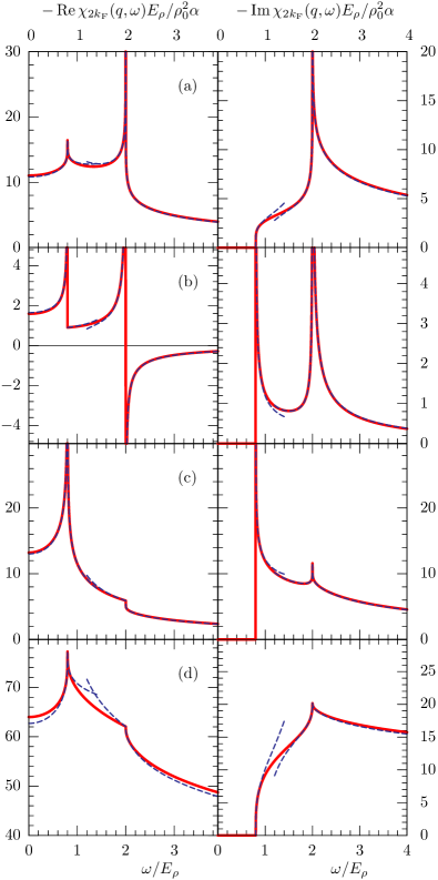
Figure 1: (Color online) Real and imaginary parts of $\chi_{2k_{\mathrm{F}}}(q,\omega)$ as a function of frequency (filled red lines) for $q=0$, $v_{\sigma}/v_{\rho}=.4$, and (a) $K_{\rho}=1$, $K_{\sigma}=.4$, (b) $K_{\rho}=.4$, $K_{\sigma}=.2$, (c) $K_{\rho}=.4$, $K_{\sigma}=1$ and (d) $K_{\rho}=.8$, $K_{\sigma}=1$. The last case corresponds to the repulsive Hubbard model away from half filling. The comparison with the approximate expressions from Eqs. (13) and (14) are also shown (dashed blue lines). The charge energy is defined as $E_{\rho}=k_{\mathrm{F}}v_{\rho}$

More schematically, the singular behavior is given by

$$\chi^{0}_{2k_{\mathrm{F}}}(q,\omega) \sim|\omega^{2}-v_{\rho}^{2}q^{2}|^{\frac{K_{\rho}}{2}+K_{\sigma}-1}+\text{const}$$ (15)

$$\chi^{0}_{2k_{\mathrm{F}}}(q,\omega) \sim|\omega^{2}-v_{\sigma}^{2}q^{2}|^{\frac{K_{\sigma}}{2}+K_{\rho}-1}+\text{const}.$$ (16)

for $\omega\approx\pm v_{\rho}q$ and $\omega\approx\pm v_{\sigma}q$ respectively. In Fig. 1 we show plots of the real and imaginary parts of $\chi_{2k_{\mathrm{F}}}(q,\omega)$ (as defined in Eq. (5)) as a function of $\omega$, for a fixed value of $q=0$ and for a ratio of velocities $v_{\sigma}/v_{\rho}=.4$. The frequency is expressed in units of the charge energy $E_{\rho}=v_{\rho}k_{\mathrm{F}}$. The singular behavior near charge and spin singularities (13) and (14) is also shown. There will be a divergence near the charge singularity for $\frac{K_{\rho}}{2}+K_{\sigma}<1$ and a dip otherwise. In cases where a divergence is present, it can be accompanied by a change of sign when the frequency goes through the singularity ($\omega<v_{\rho}q$ to $\omega>v_{\rho}q$) as in shown Fig. 1(b) (real part) [contrary to Fig. 1(a)]. This is due to the imaginary exponential factors in Eq. (13), and it is easy to see that the condition to be fulfilled for a change of sign is $\frac{K_{\rho}}{2}+K_{\sigma}-1<-\frac{1}{2}$. There are analogous results for the spin singularity at $\omega\approx\pm v_{\sigma}q$. Notice that the presence of prefactors and additional constants in Eq. (13) and (14) may change dips into peaks of finite height, as is the case of the singular behavior near the spin singularity of the real part of $\chi_{2k_{\mathrm{F}}}$ in Fig. 1(a), and near the charge singularity of the imaginary part of $\chi_{2k_{\mathrm{F}}}$ in Fig. 1(c) and (d).

In the figure the four possible cases are presented. In Fig. 1(a) we observe a divergence in the charge singularity in the imaginary part; in (b) both singularities are divergent; in (c) the divergence is in the spin singularity and in (d) there are no divergences. One especially important case is the SU(2) symmetric line $K_{\sigma}=1$, where the charge singularity is always finite, and the spin singularity can be divergent for $K_{\rho}<1/2$. In particular, Eq. (1) represents the low energy effective Hamiltonian for the repulsive Hubbard model away from half-filling, in which case the spin parameter flows to the fixed point $K_{\sigma}^{\ast}=1$ and $\frac{1}{2}<K_{\rho}<1$. In this situation $\chi_{2k_{\mathrm{F}}}$ shows no divergences in the spin and charge singularities, as it is depicted in Fig. 1(d).

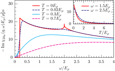
Figure 2: (Color online) Imaginary parts of $\chi_{2k_{\mathrm{F}}}(q,\omega)$ as a function of frequency for $q=0$, $v_{\sigma}/v_{\rho}=.1$, $K_{\rho}=.5$, $K_{\sigma}=1$. In the inset we observe the suppression of the correlation function under the effect of temperature (we show its behavior for fixed values of $\omega$).

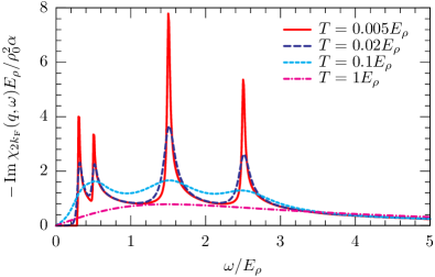
Figure 3: (Color online) Imaginary parts of $\chi_{2k_{\mathrm{F}}}(q,\omega)$ as a function of frequency for $q=k_{\mathrm{F}}/2$, $v_{\sigma}/v_{\rho}=.2$, $K_{\rho}=.4$, $K_{\sigma}=.2$. The four peak structure is the effect of taking $q\neq 0$.

V $\chi_{2k_{\mathrm{F}}}(q,\omega)$ at finite temperature

The finite temperature case is important as it tells how the singularities at $\omega=\pm v_{\sigma}q,\pm v_{\rho}q$ will be rounded with temperature. Also, if $v_{\sigma}/v_{\rho}\ll 1$ the spin-incoherent regimeFiete (2006) (defined as $v_{\sigma}k_{\mathrm{F}}\ll k_{B}T\ll v_{\rho}k_{\mathrm{F}}$) can be approached from temperatures below the spin energy, $v_{\sigma}k_{\mathrm{F}}$. As we will see below, in this limit the $2k_{\mathrm{F}}$ correlations (which may dominate the experimental signal at zero temperature) are rapidly suppressed with temperature. The presence or absence of $2k_{\mathrm{F}}$ density correlations at a given temperature has imporant implications for Coulomb dragFiete et al. (2006) and voltage noiseFiete and Kindermann (2007) on a metallic device in close proximity to a quantum wire. Moreover, the temperature dependence of these quantities can reveal spin-incoherent Luttinger liquid behavior.Fiete (2006)

Unfortunately, we were not able to obtain a simple analytical form for the Fourier transform of the finite temperature density correlations (4). However, we were able to extract some approximate results and study the Fourier transform numerically.

We study the temperature dependence of the Fourier transform using the result (30),

$$\operatorname{Im}\chi^{\text{ret}}(q,\omega)=-\int\frac{dq^{\prime}}{2\pi}\int\frac{d\epsilon^{\prime}}{\pi}[n_{\text{B}}(\epsilon^{\prime}-\omega)-n_{\text{B}}(\epsilon^{\prime})]\\ \times\operatorname{Im}\chi_{\sigma}^{\text{ret}}(q-q^{\prime},\omega-\epsilon^{\prime})\operatorname{Im}\chi_{\rho}^{\text{ret}}(q^{\prime},\epsilon^{\prime}),$$ (17)

whereGiamarchi (2004)

$$\chi^{\text{ret}}_{\sigma}(q,\omega)=-\frac{\sin(\pi K_{\sigma}/2)\rho_{0}\alpha^{2}}{v_{\sigma}}\left(\frac{2\pi T\alpha}{v_{\sigma}}\right)^{K_{\sigma}-2}\\ \times B\left(-i\frac{\omega-v_{\sigma}k}{4\pi T}+\frac{K_{\sigma}}{4},1-\frac{K_{\sigma}}{2}\right)\\ \times B\left(-i\frac{\omega+v_{\sigma}k}{4\pi T}+\frac{K_{\sigma}}{4},1-\frac{K_{\sigma}}{2}\right)$$ (18)

and $B$ is the beta function. A similar expression exists for $\operatorname{Im}\chi^{\text{ret}}_{\rho}(q,\omega)$.

The behavior of the imaginary part of $\chi_{2k_{\mathrm{F}}}(q,\omega)$ as a function of $\omega$ for fixed $q$ is shown in Figs. 2 (for $q=0$) and 3 (for $q\neq 0$) for two different sets of parameters. Notice that the four peak structure of Fig. 3 is the effect of taking $q\neq 0$. We observe that the main effect of finite temperature is 2-fold: i) there is a suppression of the whole $2k_{\mathrm{F}}$ correlation function, and ii) temperature just rounds the singularities at $\omega=\pm v_{\sigma}q,\pm v_{\rho}q$ for $|\omega-v_{\sigma}q|<\pi Tv_{\rho}/v_{\sigma}$, while for larger $|\omega-v_{\sigma}q|$ the temperature effects are minimal.

VI Summary

We have given an exact closed form expression for the zero temperature Fourier transform of the $2k_{\mathrm{F}}$ component of the retarded density-density correlation function in a Luttinger liquid with different velocities of spin and charge oscillations and arbitrary stiffness constants. Additionally, we have found approximate expressions near the collective spin and charge mode singularities that essentially take the form of power laws, whose exponents depend in a simple manner on $K_{\rho}$ and $K_{\sigma}$. We also compared these approximations directly with the exact result.

We were not able to find an exact result for the finite temperature case, but we were able to evaluate the Fourier transform numerically and determine some approximate results. One important result of the analysis is that the $2k_{\mathrm{F}}$ oscillations are dramatically (exponentially) suppressed with temperature when the spin and charge velocities are very different. This has implications for observable quantities that depend on the $2k_{\mathrm{F}}$ density correlations, such as Coulomb drag or voltage fluctuations on a metallic gate proximate to a quantum wire.

Appendix A Coefficients of expansions near charge and spin singularities

The coefficients $A_{\rho/\sigma}$ and $B_{\rho/\sigma}$ appearing in (13) and (14) are given by

$$A_{\rho} =\frac{\Gamma\left(1-K_{\sigma}-\frac{K_{\rho}}{2}\right)}{\Gamma\left(\frac{K_{\rho}}{2}\right)}F\left(K_{\rho}+K_{\sigma}-1,\frac{K_{\rho}+K_{\sigma}-1}{2},K_{\rho}+K_{\sigma}-1;r\right),$$ (19)

$$B_{\rho} =\frac{\Gamma\left(1-\frac{K_{\rho}+K_{\sigma}}{2}\right)\Gamma\left(\frac{K_{\rho}}{2}+K_{\sigma}-1\right)}{\Gamma\left(\frac{K_{\sigma}}{2}\right)\Gamma\left(K_{\rho}+K_{\sigma}-1\right)}F\left(\frac{K_{\rho}}{2},\frac{K_{\rho}+K_{\sigma}-1}{2},K_{\rho}+K_{\sigma}-1;r\right),$$ (20)

$$A_{\sigma} =\frac{\Gamma\left(1-K_{\rho}-\frac{K_{\sigma}}{2}\right)}{\Gamma\left(\frac{K_{\sigma}}{2}\right)},$$ (21)

$$B_{\sigma} =\frac{\Gamma\left(1-\frac{K_{\rho}+K_{\sigma}}{2}\right)\Gamma\left(\frac{K_{\sigma}}{2}+K_{\rho}-1\right)}{\Gamma\left(\frac{K_{\rho}}{2}\right)\Gamma\left(K_{\rho}+K_{\sigma}-1\right)}F\left(\frac{K_{\rho}+K_{\sigma}-1}{2},\frac{K_{\sigma}}{2}+K_{\rho}-1,K_{\rho}+K_{\sigma}-1;r\right),$$ (22)

where $F$ is the Gauss Hypergeometric function (sometimes written ${}_{2}F_{1}$).

Appendix B General formula for Fourier transform of $2k_{\mathrm{F}}$ response function

The $2k_{\mathrm{F}}$ part of the density-density correlation function (4) can be expressed as

$$\chi(x,\tau)=\chi_{\sigma}(x,\tau)\chi_{\rho}(x,\tau),$$ (23)

where we use definition of the Fourier transform

$$\chi(q,i\nu)=\int_{-\infty}^{\infty}dx\int_{0}^{\beta}d\tau\,e^{i(\nu\tau-qx)}\chi(x,\tau).$$ (24)

to write $\chi(q,i\nu)$ as a convolution of terms

$$\chi(q,i\nu)=\frac{1}{\beta}\sum_{\omega_{n}}\int\frac{dq^{\prime}}{2\pi}\chi_{\sigma}(q-q^{\prime},i\nu-i\omega_{n})\chi_{\rho}(q^{\prime},i\omega_{n}).$$ (25)

Using the spectral representation

$$\chi(q,z)=-\frac{1}{\pi}\int d\epsilon\frac{\operatorname{Im}\chi^{\text{ret}}(q,\epsilon)}{z-\epsilon},$$ (26)

one finds

$$\chi(q,i\nu)=\frac{1}{\beta}\sum_{\omega_{n}}\int\frac{dq^{\prime}}{2\pi}\int\frac{d\epsilon_{1}}{\pi}\int\frac{d\epsilon_{2}}{\pi}\\ \times\frac{\operatorname{Im}\chi_{\sigma}^{\text{ret}}(q-q^{\prime},\epsilon_{1})}{i\nu-i\omega_{n}-\epsilon_{1}}\frac{\operatorname{Im}\chi_{\rho}^{\text{ret}}(q^{\prime},\epsilon_{2})}{i\omega_{n}-\epsilon_{2}},$$ (27)

where the outer sum can be evaluated with standard complex integration:

$$\frac{1}{\beta}\sum_{\omega_{n}}\frac{1}{i\nu-i\omega_{n}-\epsilon_{1}}\frac{1}{i\omega_{n}-\epsilon_{2}}=-\frac{n_{\text{B}}(\epsilon_{2})-n_{\text{B}}(-\epsilon_{1})}{i\nu-\epsilon_{2}-\epsilon_{1}}.$$ (28)

Therefore, one finds

$$\chi(q,i\nu)=-\int\frac{dq^{\prime}}{2\pi}\int\frac{d\epsilon_{1}}{\pi}\int\frac{d\epsilon_{2}}{\pi}\frac{n_{\text{B}}(\epsilon_{2})-n_{\text{B}}(-\epsilon_{1})}{i\nu-\epsilon_{1}-\epsilon_{2}}\\ \times\operatorname{Im}\chi_{\sigma}^{\text{ret}}(q-q^{\prime},\epsilon_{1})\operatorname{Im}\chi_{\rho}^{\text{ret}}(q^{\prime},\epsilon_{2}),$$ (29)

from which the analytical continuation $i\nu\to\omega+i\delta$ can readily to be done to yield

$$\operatorname{Im}\chi(q,\omega)=-\int\frac{dq^{\prime}}{2\pi}\int\frac{d\epsilon^{\prime}}{\pi}[n_{\text{B}}(\epsilon^{\prime}-\omega)-n_{\text{B}}(\epsilon^{\prime})]\\ \times\operatorname{Im}\chi_{\sigma}^{\text{ret}}(q-q^{\prime},\omega-\epsilon^{\prime})\operatorname{Im}\chi_{\rho}^{\text{ret}}(q^{\prime},\epsilon^{\prime}).$$ (30)

References

- Giamarchi (2004) T. Giamarchi, Quantum Physics in One Dimension (Oxford University Press, Oxford, 2004).
- Schwartz et al. (1998) A. Schwartz, M. Dressel, G. Grüner, V. Vescoli, L. Degiorgi, and T. Giamarchi, Phys. Rev. B 58, 1261 (1998).
- Bockrath et al. (1999) M. Bockrath, D. H. Cobden, J. Lu, A. G. Rinzler, R. E. Smalley, L. Balents, and P. L. Mceuen, Nature (London) 397, 598 (1999).
- Yao et al. (1999) Z. Yao, H. W. C. Postma, L. Balents, and C. Dekker, Nature (London) 402, 273 (1999).
- Auslaender et al. (2005) O. M. Auslaender, H. Steinberg, A. Yacoby, Y. Tserkovnyak, B. I. Halperin, K. W. Baldwin, L. N. Pfeiffer, and K. W. West, Science 308, 88 (2005).
- Haldane (1981) F. D. M. Haldane, J. Phys. C 14, 2585 (1981).
- Haldane (1980) F. D. M. Haldane, Phys. Rev. Lett. 45, 1358 (1980).
- Voit (1995) J. Voit, Rep. Prog. Phys. 58, 977 (1995).
- Cross and Fisher (1979) M. C. Cross and D. S. Fisher, Phys. Rev. B 19, 402 (1979).
- Schulz and Bourbonnais (1983) H. J. Schulz and C. Bourbonnais, Phys. Rev. B 27, 5856 (1983).
- Voit (1993) J. Voit, Phys. Rev. B 47, 6740 (1993).
- Meden and Schönhammer (1992) V. Meden and K. Schönhammer, Phys. Rev. B 46, 15753 (1992).
- Schönhammer and Meden (1993) K. Schönhammer and V. Meden, Electron Spectrosc. Relat. Phenom. 62, 225 (1993).
- Nakamura and Suzumura (1997) N. Nakamura and Y. Suzumura, Prog. Theor. Phys. 98, 29 (1997).
- Kivelson et al. (2003) S. A. Kivelson et al., Rev. Mod. Phys. 75, 1201 (2003).
- Orignac and Citro (2006) E. Orignac and R. Citro, Phys. Rev. A 73, 063611 (2006).
- Fiete et al. (2006) G. A. Fiete, K. Le Hur, and L. Balents, Phys. Rev. B 73, 165104 (2006).
- Pustilnik et al. (2003) M. Pustilnik, E. G. Mischenko, L. I. Glazman, and A. V. Andreev, Phys. Rev. Lett. 91, 126805 (2003).
- Fiete and Kindermann (2007) G. A. Fiete and M. Kindermann, Phys. Rev. B 75, 035336 (2007).
- Cheianov and Zvonarev (2004) V. V. Cheianov and M. B. Zvonarev, Phys. Rev. Lett. 92, 176401 (2004).
- Fiete and Balents (2004) G. A. Fiete and L. Balents, Phys. Rev. Lett. 93, 226401 (2004).
- Fiete (2006) G. A. Fiete (2006), (To appear in Rev. Mod. Phys.), eprint cond-mat/0611597.
- Orgad (2001) D. Orgad, Phil. Mag. B 81, 375 (2001).
- Peskin and Schroeder (1995) M. E. Peskin and D. V. Schroeder, An introduction to quantum field theory (Addison-Wesley, Massachusettes, 1995).
- Bateman Manuscript Proyect (1953) Bateman Manuscript Proyect, Higher Transcendental Functions (McGraw-Hill Book Company Inc., New York, 1953), vol. 1.
- Slater (1966) L. J. Slater, Generalized Hypergeometric Functions (Cambridge University Press, Cambridge, 1966).
- Olsson (1964) O. M. Olsson, J. Math. Phys. 5, 420 (1964).
- Gradshteyn and Ryzhik (1980) A. Gradshteyn and R. Ryzhik, Tables of integrals series and products (Academic Press, New-York, 1980).